21st-century climate change around Kangerlussuaq, west Greenland: From the ice sheet to the shores of Davis Strait

ABSTRACT

Using regional climate-model runs with a horizontal resolution of 5.5 km for two future scenarios and two time slices (representative concentration pathway [RCP] 4.5 and 8.5; 2031–2050 and 2081–2100) relative to a historical period (1991–2010), we study the climate change for the Qeqqata municipality in general and for Kangerlussuaq in particular. The climate-model runs are validated against observations of temperature and surface mass balance and a reanalysis simulation with the same model setup as the scenario runs, providing high confidence in the results. Clear increases in temperature and precipitation for the end of the 21st century are shown, both on and off the ice sheet, with an off–ice sheet mean annual temperature increase of 2.5–3°C for the RCP4.5 scenario and 4.8–6.0°C for the RCP8.5 scenario, and for precipitation an increase of 20–30% for the RCP4.5 scenario and 30–80% for the RCP8.5 scenario. Climate analogs for Kangerlussuaq for temperature and precipitation are provided, indicating that end-of-the-century Kangerlussuaq mean annual temperature is comparable with temperatures for the south of Greenland today. The extent of glacial retreat is also estimated for the Qeqqata municipality, suggesting that most of the ice caps south of the Kangerlussuaq fjord will be gone before the end of this century. Furthermore, the high-resolution runs are compared with an ensemble of six models run at a 50 km resolution, showing the need for high-resolution model simulations over Greenland.

KEYWORDS:

• Climate change
• regional climate modeling
• surface mass balance
• Kangerlussuaq

Introduction

The climate of the Arctic is in rapid transition, with Greenland and its ice sheet already seeing the impacts of rising regional temperatures, including ice loss of approximately 234 ± 20 Gt yr⁻¹ since 2003, contributing about 0.7 mm yr⁻¹ to the sea level (Barletta, Sørensen, and Forsberg 2013; Shepherd et al. 2012). Future climate change is likely to continue to have a significant impact on both the ice sheet and adjacent areas, with a consequent effect on global and regional sea levels. The Greenland Ice Sheet contains about 10 percent of global freshwater reserves, sufficient to raise sea level by an average of about 7 m should it melt completely, meaning that the future change of the ice mass is of global concern. Locally, impacts from increasing amounts of ice-sheet mass loss, as well as regional climate change with increased extreme weather events and changes in long-term climate, have implications for infrastructure, industry, and agriculture. Recent work by Christensen et al. (2016) used a combination of global climate models from CMIP5 and high-resolution regional downscaling to determine what the future climate of Greenland will be like and how local inhabitants can best prepare for and adapt to, for example, permafrost degradation, enhanced flooding related to extreme weather events, and high melt rates (Mikkelsen et al. 2016), as well as the implications for fisheries, hunting, and agriculture. Climate change can have unpredictable consequences as, for example, in Greenland, where the length of the growing season is expected to increase during the 21st century, but there are also indications that periods of drought will increase. Both of these processes will affect agricultural productivity, and therefore proper technical solutions will be required to expand current crop production and livestock management, especially in regions further north in Greenland than are currently farmed. The habitable parts of Greenland, with the exception of the most southern locations, are also subject to changes in permafrost conditions. This is particularly an issue around Kangerlussuaq and more generally in the Qeqqata municipality located in the discontinuous to continuous permafrost region of west Greenland (Christiansen and Humlum 2000). Here, the permafrost thaw potential has been classified as high (Daanen et al. 2011), which is confirmed by the results presented in Christensen et al. (2016). For these reasons, assessing the future climate of Greenland on both a regional and local scale is important both for infrastructure planning and future development as well as to more widely to identify processes and feedbacks that may affect ice-sheet mass loss.

In this study we focus on a well-populated region (by Greenland standards), with a number of infrastructural challenges on land and a significant area of ice sheet. The region around Kangerlussuaq and Sisimiut, Qeqqata municipality, is home to approximately 10,000 people, about one-fifth of the population of Greenland. The region also has a number of long-running observational datasets both on and off the ice sheet (Oerlemans and Vugts 1993; van den Broeke, Smeets, and van de Wal 2011; van de Wal et al. 2012; van de Wal and Russell 1994). These are useful to assess the performance of models and to allow the development of process-based estimates of expected change. Global climate models (GCMs) are run at institutes worldwide to assess the large-scale effects of global warming and make future projections. With the relatively coarse resolution (100–200 km) of the state-of-the-art GCMs currently in use, Greenland is often modeled as an island covered by ice without accounting for the significant processes occurring at the ice-sheet surface (e.g., Cullather et al. 2014). To resolve the finer details that are more useful for prescribed regions or for complex process studies, regional climate models (RCMs) are useful for dynamically down-scaling these climate projections. In Greenland, the RCMs RACMO (e.g., Ettema et al. 2009; Noël et al. 2016), MAR (e.g., Fettweis et al. 2017, 2013), and PolarMM5 (Burgess et al. 2010) as well as HIRHAM5 (Lucas-Picher et al. 2012) have previously been used for climate research. A comparison of the performance of early versions of these RCMs in Rae et al. (2012) showed some differences in performance. However, analysis by Mottram et al. (2017) and Vernon et al. (2013) shows that these RCMs produce similar values for surface mass balance over the ice sheet as a whole, although with some significant differences in the components of mass balance and in the spatial distribution of these components (e.g., Langen et al. 2015; Van As et al. 2014), partly attributable to different model resolution as well as different ice masks and potentially different parameterization schemes. Here, we focus on validating the HIRHAM5 simulations against observations, excluding a comparison with previous high-resolution downscalings.

More recently, Langen et al. (2015) used a detailed and updated version of RCM HIRHAM5 (Christensen et al. 2006) with high resolution (5.5 km), driven by reanalysis data (ERA-Interim; Dee et al. 2011) covering the whole of Greenland, to estimate the changes in ice-sheet surface mass balance for the drainage basin linked to the Godthåbsfjord. The HIRHAM5 model has been further refined with a number of additions that include a more sophisticated snow scheme suited to accurately capturing albedo feedbacks and processes within the snowpack (see Langen et al. 2017 for details). Also note that the HIRHAM5 model, as with most RCMs, has a fixed topography and does not account for feedback caused by surface elevation changes.

In this study we use the same model setup as in Langen et al. (2017), and force the model with the EC-Earth GCM (Hazeleger et al. 2012) at the lateral boundaries for two different future scenarios (representative concentration pathway [RCP] 4.5 and RCP8.5) and with the historical emissions forcing (Mottram et al. 2017). We run the model transiently for three time periods (1991–2010, 2031–2050, 2081–2100). Comparing the two later time periods with the former, a control period that overlaps with the ERA-Interim reanalysis experiments, we can thus project climate change in the Qeqqata region, both off and on the glacier.

The performance of the HIRHAM5 RCM, driven by the ERA-Interim reanalysis, has been fully evaluated by Langen et al. (2015, 2017) and by Mottram et al. (2017), showing that the ice sheet is well represented during present-day conditions with a surface mass balance in the ablation area close to observations but with an underestimation of the interannual variability of the number of melt days. We here use weather station observations to also evaluate the performance of the HIRHAM5 when forced with the EC-Earth historical scenario in order to validate the use of the EC-Earth GCM as forcing at the lateral boundaries. This gives us valuable insight to interpret the output of the model when forced with future simulations from EC-Earth.

Data

Observations

Monthly means of observed temperature are collected for five locations within the region of study. Cappelen (2016) provided station measurements for Sisimiut and Kangerlussuaq (see Figure 1). Data for the other three locations are as described by van den Broeke et al. (2011), using automatic weather stations (AWS) on the ice sheet (see Figure 1). These AWS are at surface elevations of 490 (S5), 1,020 (S6), and 1,520 m a.s.l. (S9) at distances of 6, 38, and 88 km from the ice-sheet margin, respectively.

Figure 1. Model orography for the full model domain (a, top) and for the Qeqqata municipality (b, bottom). Sea points are given in blue, glacier-free land points in green/brown, and glacier points in white with added surface elevation contour lines. Also shown are the location of five villages and the S5, S6, and S9 weather stations (van de Wal et al. 2005). Three ice caps are given by letters A, B, and C and are named Qapiarfiup Sermia, Sukkertoppen Ice Cap, and Tasersiap Sermia, respectively. The fjord Kangerlussuaq is given by the letter D, and Watson River by the letter E. The Kangerlussuaq drainage basin is shown in magenta. The location of surface mass balance stations are given as red dots within two black ellipses

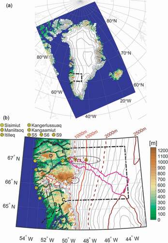
Because the runoff of from the ice sheet is important for the local infrastructure (Mikkelsen et al. 2016), we estimate the amount of glacial freshwater input to the Watson River. For this calculation we use the drainage basin definition (see Figure 1) from Lindbäck et al. (2014, 2015), who used a single-direction flow algorithm and surface analysis in order to derive a drainage catchment on the hydraulic potential surface.

Models

HIRHAM5 (Christensen et al. 2006) is an RCM consisting of the dynamic core of the numerical weather forecast model HIRLAM together with the physics scheme from the GCM ECHAM. Compared with the HIRHAM5 version described in Christensen et al. (2006), a dynamic snow/ice scheme together with an updated snow/ice albedo scheme have been included in the model runs used in this study (see Langen et al. 2015, 2017 for details).

In this study, the HIRHAM5 RCM is forced at the boundaries by EC-Earth (Hazeleger et al. 2012). The Earth system model (ESM) EC-Earth is based on the operational seasonal forecast system of the European Centre for Medium-Range Weather Forecasts (ECMWF), but with an interactive atmosphere-ocean-sea ice coupling applied across the entire globe. When compared to other coupled models with similar complexity, the model performs well in simulating tropospheric fields and dynamic variables (Hazeleger et al. 2012). However, EC-Earth has a 2°C cold bias over the Arctic with an overestimation of sea-ice extent and thickness (Koenigk et al. 2013).

Five twenty-one-year time slices, dynamically downscaling the EC-Earth output over Greenland, have been performed. In these downscalings, HIRHAM5 is forced by EC-Earth only at the boundaries every six hours and with sea-ice cover and sea-surface temperatures once per day within the domain. The periods include a historical period (1990–2010), two periods for the RCP4.5 scenario (2030–2050 and 2080–2100), and two periods for the RCP8.5 scenario (2030–2050 and 2080–2100). The first year of each time slice was used as a spin-up and therefore not used, resulting in five twenty-year time slices used in this study. In addition to the online one-year spin-up of atmospheric conditions, we included an offline spin-up of about 100 years, looping over the first decade of each individual time-slice experiment, with focus on the subsurface conditions (Langen et al. 2017). We compare the EC-Earth forced regional downscalings for the historical period 1991–2010, with a simulation forced by ERA-Interim (ERA-I; Dee et al. 2011) but otherwise identical in setup (see Langen et al. 2017).

The HIRHAM5 simulations are validated using the observations given earlier. We also compare our high-resolution runs with a model ensemble consisting of all available CORDEX (Jones, Giorgi, and Asrar 2011) runs for the Artic domain (ARC-44), with a horizontal resolution of 50 km (see Table 1). The CORDEX database includes simulations from four GCMs downscaled with three regional climate models, including the simulations discussed in this article. With a horizontal resolution of 50 km, the CORDEX runs for the Arctic domain are not able to give a reasonable view of the nonglacier areas of Greenland having a clear influence from the ice sheet. We therefore only use the CORDEX data in validating the 5.5 km runs on the ice sheet.

Table 1. List of all available CORDEX ARC-44 GCM-driven simulations used for comparison with the high-resolution run for Greenland

RCMs	GCMs				Reference
	CCCma-CanESM2	ICHEC-EC-EARTH	NCC-NorESM1-M	MPI-M-MPI-ESM-LR
DMI-HIRHAM5		x			Christensen et al. (2006)
SMHI-RCA4	x	x	x	x	Samuelsson et al. (2011)
MGO-RRCM				x	Shkolnik et al. (2007)

Results

Model validation

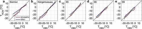
Since EC-Earth is a dynamically self-consistent climate model, with variability being out of phase with reality, the regional downscaling over Greenland has to be compared against observations in a statistical sense and not compared month by month. A simple but efficient method is quantile-quantile plots, where model data and observations are ranked individually so that their quantiles are plotted against each other. Figure 2 gives quantile-quantile plots of monthly mean temperatures for the historical EC-Earth run as a function of observed monthly mean temperatures. Note that the weather station data do not cover the full 1991–2010 period. Also shown are monthly mean temperatures taken from the ERA-I run used in Langen et al. (2017) and Mottram et al. (2017), and we see that the EC-Earth historical downscaling has a close match to observations for monthly mean temperatures, both off (panels A and B) and on (panels C, D, and E) the ice sheet, and it performs at the same level as the ERA-I downscaling.

Figure 2. Quantile-quantile plots of monthly mean temperatures (model vs. observations). The global climate model (GCM)-driven historical simulation is shown in red while the ERA-I-driven simulation is shown in blue. Each panel represents a specific location and time period. (a) Sisimiut 1991–2010, (b) Kangerlussuaq 1991–2010, (c) weather station S5 1993–2010, (d) weather station S6 1995–2010, and (e) weather station S9 2000–2010

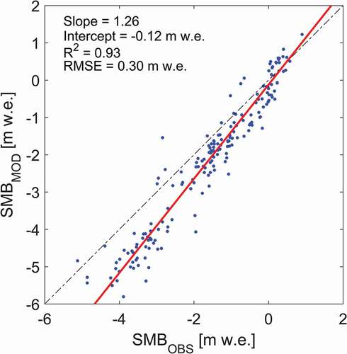
Machguth et al. (2016) compiled an extensive set of surface mass balance (SMB) observations, with a total of 180 observational records within the Qeqqata municipality, overlapping in time with our experiment (cf. the red dots in the right panel of Figure 1). The individual observations have a very limited time span (from two months to two years), making the observations difficult to compare with the dynamically self-consistent GCM-driven simulations. Figure 3 therefore compares the observed SMBs with the ERA-I-driven simulation SMB only. Although the model shows a clear overestimation (26 percent on average based on the slope of an orthogonal least squares fit) of the rate of ice loss, the linear correlation between the 180 data points is relatively high and the RMSE value for the fitted line is relatively low.

Figure 3. Scatter plot of observed and modeled surface mass balance (SMB) at 180 locations in Qeqqata municipality. An orthogonal linear fit to all data is shown in red together with statistics for the fit in the top left. Note that observations (and model data) cover uneven time periods, ranging from two months to as much as two years

Over the ice sheet, we make area-weighted sums of snowmelt and total runoff for grid points located within the Kangerlussuaq drainage basin (Lindbäck et al. 2014, 2015). As shown in Figure 4, we see a clear difference between the historical EC-Earth-driven run (black) and the ERA-I-driven run (green). For snowmelt, the ERA-I run has an average of 7.3 Gt yr⁻¹ for 1991–2010, while the EC-Earth run has an average of 4.8 Gt yr⁻¹. This underestimation of melt is a consequence of a continental and North Atlantic summer cold bias in the driving EC-Earth present-day simulation (Hazeleger et al. 2012). This cold bias leads to downward fluxes of energy (particularly in downwelling longwave radiation) that are smaller than those in the ERA-I-driven run during the melting season (not shown). Nevertheless, the near-surface summer air temperatures in the EC-Earth-driven run at the on-ice stations (Figure 2C–E) are similar to or only slightly lower than those in the ERA-I-driven run because the near-surface air temperatures are kept close to the temperature of the melting surface. Why no cold bias is seen for the warm period in Figure 2B is unclear at this moment.

Figure 4. Change in snowmelt (solid lines) and total surface runoff (dashed lines) for the Kangerlussuaq drainage basin for the historical period (black), representative concentration pathway [RCP] 4.5 (blue), and RCP8.5 (red). Also shown, in green, is snowmelt and runoff for the ERA-I-driven run for 1980–2014

Climate change off the ice sheet

Figure 5 shows change in temperature (panels A–D) and change in precipitation (panels E–H) for the west part of Qeqqata municipality relative to the 1991–2010 historical period. The change in temperature is relatively uniform for all four individual scenario periods. This we mostly attribute to the similarity of the ice-free surfaces and the vicinity of large-scale homogeneous sources of heat (the ocean) and the ice sheet (cold buffer). At the annual time scale, this large-scale driver of change dominates. Certain topographically induced features show up somewhat more clearly at seasonal or shorter time scales (not shown). As shown in Table 2, we project an increase in annual temperature at the end of the 21st century of about 3°C for the RCP4.5 scenario and an increase of about 5.5°C for the RCP8.5 scenario for west Greenland (global mean values of annual temperature changes for EC-Earth are 2°C and 4°C for RCP4.5 and RCP8.5, respectively; i.e., the regional values using HIRHAM5 are 50% and 40% above the global means for RCP4.5 and RCP8.5, respectively). This increase in temperature will intensify the local/regional water cycle, and in line with the general expected increase in precipitation in the polar regions, Qeqqata will also likely experience an overall increase in precipitation. This change in precipitation is less uniform, as seen in Figure 5E–H, with an intensification of the present-day pattern of rainfall. This pattern largely reflects the rugged topography of the region, with the Sukkertoppen Ice Cap and Tasersiap Sermia catching much of the precipitation and Kangerlussuaq lying in its rain shadow. For Kangerlussuaq, at the end of the century we project an increase in precipitation of up to about 300 mm yr⁻¹, with the largest contribution the result of an increase in rainfall. A general shift in the rain/snowfall ratio is seen over most of the land areas of Greenland (not shown, Christensen et al. 2016).

Table 2. Changes in annual mean temperature and precipitation relative to the 1991–2010 historical period for five locations in Qeqqata

Location	RCP4.5 2031–2050		RCP4.5 2081–2100		RCP8.5 2031–2050		RCP8.5 2081–2100
	ΔT (°C)	ΔP (%)	ΔT (°C)	ΔP (%)	ΔT (°C)	ΔP (%)	ΔT (°C)	ΔP (%)
Sisimiut	0.9	11	3.0	28	1.9	15	6.0	40
Kangerlussuaq	0.9	17	2.4	34	2.0	8	4.8	81
Maniitsoq	0.8	12	2.9	23	1.8	16	5.3	34
Kangaamiut	0.8	16	2.9	27	1.8	21	5.5	34
Itilleq	0.9	15	2.8	34	1.9	17	5.6	58

Figure 5. Change in annual temperature and precipitation for western Qeqqata. (a, e) representative concentration pathway [RCP] 4.5 2031–2050 change relative to 1991–2010; (b, f) RCP4.5 2081–2100 change relative to 1991–2010; (c, g) RCP8.5 2031–2050 change relative to 1991–2010; and (d, h) RCP8.5 2081–2100 change relative to 1991–2010. See the Figure 1 caption for an explanation of the yellow markers. The white line outlines the ice sheet

Another way to study the change in temperature and precipitation is to use future climate analogs for these variables. Climate analogs in this part of Greenland can be seen as an attempt to identify what the future climatic setting of the region will look like. Taking the area around Kangerlussuaq as representative for the landscape in this continental climate setting, we can search for locations in present-day climate that already look like the projected future for Kangerlussuaq. Figure 6 shows the annual mean climate analog for Kangerlussuaq for the RCP8.5 scenario. For temperature (panel A), the mid-century analog (orange) is identified with locations close to the Nuuk region, while the end of the century analog (red) is closer to the present-day climate of the Qaqortoq region. Thus, the analog first moves toward the ocean outward from Kangerlussuaq fjord and then southward as the temperature continues to increase. For precipitation (Figure 6B), however, the analog is moving northward and closer to the sea where the annual precipitation amount is about 300 mm higher than the current value for Kangerlussuaq. This is seen as a change from the very dry, Arctic desert-like conditions around Kangerlussuaq to wetter locations, which today can be found north of Kangerlussuaq, where a moist gradient is found seaward of Kangerlussuaq and in particular toward Disko Bay.

Figure 6. Climate analogs for temperature (a) and precipitation (b) for grid points having an elevation within 200 m compared to the grid point representing Kangerlussuaq using the representative concentration pathway [RCP] 8.5 scenario only. For temperature, the orange color represents areas that for the 1991–2010 historical period have annual mean temperatures close to (±0.25°C) the annual mean temperature of Kangerlussuaq for the RCP8.5 scenario 2031–2050. Similarly, red color is for the RCP8.5 2081–2100 period. For precipitation, the interval is ±25 mm yr⁻¹. The yellow symbols (from north to south) mark the location of Aasiaat, Kangerlussuaq, Nuuk, and Qaqortoq

While agriculture may extend into these northern regions as a result of warming, the complexity of the climate analogs being quite different for temperature and precipitation suggests that the future conditions in the region will be far different than those currently experienced in the south of Greenland, where agriculture is currently largely confined.

Climate change on the ice sheet

As seen in Figure 4, melt and runoff rates intensify in both scenarios for the Kangerlussuaq drainage basin. The increases are rather modest (~35% for melt and ~38% for runoff in RCP4.5, with similar values for RCP8.5, 36% and 42%, respectively) in the 2031–2050 period, but become much larger toward the end of the century (~67% and ~165% for melt and 70% and 178% for runoff in the RCP4.5 and RCP8.5 runs, respectively). Comparing the end-of-century changes in temperature from the previous section with end-of-century melt rates, we get 22 percent °C⁻¹ (67%, 3.0°C) for RCP4.5 and 30 percent °C⁻¹ (165%, 5.5°C) for RCP8.5. These small-area totals agree well with the Greenland-wide total of 30 percent °C⁻¹ found by Fettweis et al. (2008). With average melt and runoff rates doubled or tripled in the RCP8.5 scenario, massive melt and flooding events such as those affecting the Watson River in 2012 (Mikkelsen et al. 2016) will become quite common. Even in the RCP4.5 scenario, several spikes comparable to the ERA-I-driven 2012 value occur when taking into account the 2.4 Gt yr⁻¹ offset between the two present-day references.

In Figure 7, we compare our RCP8.5 scenario experiments (minus the historical period) with a 5.5 km horizontal resolution with an ensemble median of the currently available 50 km resolution CORDEX Arctic runs for the Qeqqata region. The change in annual precipitation is of the same magnitude for the 5.5 km simulations as for the 50 km ensemble median, but the details given by the 5.5 km simulations far exceed the 50 km median. We note in particular the clear north-south gradient in the precipitation signal for Sukkertoppen Ice Cap and neighboring east-west-oriented glaciers, seen both in the near term as well as in the end-of-century time slice. Similarly, a topographically induced local enhancement at the southern end of the Watson River drainage basin is a unique feature because of the higher resolution (compare also with Figure 1). Similar plots as in Figure 7 were also made using temperature data (not shown) showing a close resemblance between the 5.5 km simulation and the 50 km ensemble median.

Figure 7. Change in precipitation for model glacier grid points in Qeqqata using the 5.5 km simulation (a, b) compared with the ensemble median for the 50 km CORDEX Arctic runs (c, d). (a, c) representative concentration pathway [RCP] 8.5 2031–2050 change relative to 1991–2010; (b, d) RCP8.5 2081–2100 change relative to 1991–2010. The Kangerlussuaq drainage basin is shown in magenta. See the Figure 1 caption for an explanation of the yellow markers

Figure 8 shows the change in SMB for RCP4.5 (panels A and B) and for RCP8.5 (panels C and D) relative to the historical run. For the mid-century time slice (panels A and C) the change is comparable for both scenarios, with values close to −0.5 m yr⁻¹ west of 48°W. East of 48°W the SMB change is positive but close to zero. For the end-of-century time slice (panels B and D), the difference in temperature change (cf. Figure 5) and increased runoff rates (Figure 4) are clearly reflected in the SMB change. For the RCP8.5 scenario, the area with a negative change in SMB (the ablation area) is clearly expanding higher up on the ice sheet, and the low-elevation value changes by as much as −2 m yr⁻¹.

Figure 8. Change in surface mass balance for model glacier grid points in Qeqqata. (a) Representative concentration pathway [RCP] 4.5 2031–2050 change relative to 1991–2010; (b) RCP4.5 2081–2100 change relative to 1991–2010; (c) RCP8.5 2031–2050 change relative to 1991–2010; and (d) RCP8.5 2081–2100 change relative to 1991–2010. The Kangerlussuaq drainage basin is shown in magenta. See the Figure 1 caption for an explanation of the yellow markers

The effect of this drastic change in SMB on the ice sheet is estimated as shown in Figure 9. By fitting a second-degree polynomial to annual SMB values for the two time slices for the RCP8.5 scenario relative to the historical period, we estimate the cumulative change in SMB for the 2011–2100 period. Here, we interpret this cumulative change in SMB as a change in ice-sheet thickness (in a manner similar to what was done in the final sensitivity experiments in Fettweis et al. 2013). If the resulting surface lowering exceeds the ice-sheet thickness (Morlighem et al. 2014) for a specific grid cell, that grid cell is then shown as a nonglacial grid cell in Figure 9. The most clear effect of ice-sheet retreat in this region is seen for the three ice caps located south of the Kangerlussuaq fjord (Sukkertoppen Ice Cap, Tasersiap Sermia, and Qapiarfiup Sermia). Here we assume, for the sake of simplicity and illustration, that (1) changes in ice flow are negligible, such that increased outward flow is unable to counter the SMB-driven surface lowering, and (2) the area was in equilibrium during the 1991–2010 reference period. Changes in ice flow, if included, would likely decrease our estimates of surface lowering by increasing the amount of mass moved from the ice-sheet interior toward the margin. Alternatively, the 1991–2010 period was most likely not in equilibrium (Colgan, Thomsen, and Citterio 2015a) and the addition of this reference-period imbalance would further increase our surface-lowering estimates. On the Sukkertoppen Ice Cap in particular, there is little potential for increased flow to counter the SMB-driven retreat.

Figure 9. Glacial retreat in Qeqqata for the representative concentration pathway [RCP] 8.5 2081–2100 scenario relative to the 1991–2010 historical period, assuming that changes in ice flow are negligible and that the area was in equilibrium during the 1991–2010 reference period. Nonglacier grid cells during the historical period are shown in transparent green/brown colors. Glacier grid cells during the historical period that become nonglacier during the RCP8.5 scenario are shown in nontransparent green/brown colors. For grid cells that are glacier during all of the scenario period, the magenta/blue color map represents the change in elevation, while the contour lines give the elevation at the end of the 21st century. See the Figure 1 caption for an explanation of the yellow markers

Discussion

In Figure 2B (Kangerlussuaq), when comparing simulated and observed monthly mean temperatures, we note an offset for the cold period where the EC-Earth simulation is about 4°C lower than observations, but when the monthly mean temperature is above −10°C the model values show a very close match to observations. We also note that for Sisimiut (Figure 2A), located close to the sea, the slope of the ERA-I curve is relatively far from unity, suggesting a damping effect from the sea. Overall, the EC-Earth-driven run is colder than the ERA-I-driven run. This suggests that the reason for the better agreement in the EC-Earth-driven run may be for the wrong reasons; HIRHAM is unable to get very cold at a coastal grid point, unless the sea is fully ice covered.

The offset between the two present-day runs (EC-Earth historical and ERA-I driven) in Figure 4 illustrates the importance of referencing downscaled future scenarios with corresponding present-day runs. In this case we compare the EC-Earth-driven scenarios relative to the corresponding EC-Earth-driven present-day run; although, when doing so, one implicitly ignores potential nonlinearities whereby the magnitude of climate change can depend on the reference state (e.g., Boberg and Christensen 2012; Fettweis et al. 2013).

In this study we have analyzed high-resolution climate projections in detail to determine the likely future effects of climate change on the Qeqqata region of west Greenland. The detail provided by the high-resolution simulations is complemented by the consistency in the climate output by the available regional climate models for this region. This combination of CORDEX data and HIRHAM5 downscaling is particularly powerful for picking up local effects not otherwise captured. Of the higher-resolution models previously run for Greenland, the results are certainly comparable.

Given the very large area covered by glacier ice in this region it is unsurprising that many of the effects are seen initially in the glaciers of the region. In particular, the retreat and near disappearance of the small local ice caps in this region by the end of the century under the high-emissions scenario will have a substantial effect on the geography of the region. The increase in melt and runoff across the ice sheet is also likely to have a significant effect in river catchments such as the Watson River, which flows through Kangerlussuaq. This work suggests, therefore, that careful planning is necessary to ensure that infrastructure can withstand future extreme events that will likely become more common. Similarly, higher meltwater discharge into the fjords in this region may also have an effect on fisheries (e.g., Swalethorp et al. 2016) and needs to be taken into account.

There are few realistic analogs at the present day in Greenland for the warmer and relatively wetter climate around Kangerlussuaq, which suggests that narratives around the extension of agricultural productivity or naive approximations of ecosystem changes may be flawed. Much more work must be done by agronomists and ecologists to determine the likely impact of these projected changes on the ecosystem, wildlife, and the potential for agricultural development in this region. Alternatively, the retreat of the ice caps does provide much greater possibilities for the development of mineral resources, such as the Isua iron-ore mining prospect (Colgan et al. 2015b). The sustained increase in melt also provides an opportunity for the development of hydropower resources in this region that could provide significant power for both industrial and domestic applications (Ahlstrøm et al. 2008).

At the same time, it is notable that for the high-resolution simulations presented here, the changes in surface mass balance and both snow and ice melt scale linearly according to emissions. This suggests that, for surface mass loss processes at least, the impact of climate change on the ice sheet can still be mitigated by reductions in greenhouse gas emissions and/or content in the atmosphere. Finally, we should note that although we have focused on Qeqqata municipality in west Greenland, much of this study is relevant for many other areas, particularly in western Greenland. The retreat of the ice caps south of the fjord Kangerlussuaq is consistent with modeling by several groups focused on small glaciers and ice caps globally (e.g., Radić et al. 2014; Huss and Hock 2015; Marzeion, Jarosch, and Hofer 2012), suggesting that many of the small local glaciers will disappear from Greenland before the end of the 21st century, particularly under the high emissions RCP8.5 scenario.

The disappearance of these glaciers and the substantial retreat of the ablation zone in this area also pose a challenge to climate and ice-sheet models. The orography of the region will change substantially, potentially changing the local surface mass budget. In large-scale regional climate models such as HIRHAM5, the ice mask and topography are kept constant, and estimates of full Greenland surface mass balance may also therefore mislead. There are a number of conflicting errors. First, areas that become ice free are still counted within the surface mass budget. Second, lower elevation because of melting can enhance further melt as a feedback. Third, the ice-sheet surface slope may steepen because of the increased melt and precipitation, leading to enhanced orographic uplift and precipitation. Outside of uncoupled climate/ice-sheet models, these processes are not accounted for and there may therefore be significant uncertainties in SMB as a result.

The fact that the overall level of change in precipitation (see Figure 7) is a good match between the HIRHAM5 5.5 km simulations and the CORDEX 50 km median change indicates that the detailed changes in the very high-resolution simulation may offer clear added value compared to coarser-resolution simulations, particularly in the complex outline of terminating glacier outlets such as for the Watson River drainage basin. However, the low density of observations in Greenland makes it difficult to statistically assess if there is an improvement in precipitation gained from higher-resolution modeling, as suggested by, for example, Lucas-Picher et al. (2012), but assessment of high-resolution models of Europe unambiguously demonstrate a significant improvement in precipitation (e.g., Prein et al. 2015). The improvement shown by Prein et al. (2015) is attributed to improved representation of orography, an improvement that is also shown in the 5.5 km simulations for Greenland when compared with the CORDEX 50 km simulations.

Conclusion

Using observations of temperature both off and on the ice sheet together with SMB observations for validation, the 5.5 km resolution historical simulation has shown high confidence in the results. The historical simulation has been compared with four scenario runs: two mid-century runs for RCP4.5 and RCP8.5 and two end-of-century runs for RCP4.5 and RCP8.5. Changes in annual mean temperature (precipitation) for five locations are close to 1°C (10–20%) for the mid-century RCP4.5 time period and in the range 2.5–3°C (20–30%) for the end-of-century RCP4.5 scenario. For the RCP8.5 time slices, the changes in temperature (precipitation) are in the range 1.8–2°C (8–20%) and 4.8–6.0°C (30–80%) for mid-century and end-of-century, respectively.

We also searched for locations with a present-day climate comparable with the projected future for Kangerlussuaq using the RCP8.5 scenario. For temperature, the mean climate analog is found close to the Nuuk region for the mid-century period while the end-of-century analog is found in the Qaqortoq region. For precipitation, however, the analog is moving northward and closer to the sea, where the annual precipitation is about 300 mm higher than the present-day value for Kangerlussuaq. When studying climate change on the ice sheet, melt and runoff rates are found to significantly increase for the Kangerlussuaq drainage basin for both scenarios. The increase in melt is 67 percent for the end-of-century RCP4.5 scenario and 165 percent for the end-of-century RCP8.5 scenario. Corresponding values for end-of-century runoff are 70 percent and 178 percent for the RCP4.5 and RCP8.5, respectively, indicating more frequent massive melt and flooding events. Furthermore, when comparing the 5.5 km simulations with available 50 km CORDEX scenario simulations for precipitation on the ice sheet, similar levels of change were found on large scales, but the details given by the 5.5 km simulation suggest added value compared to coarser-resolution simulations.

The future change in SMB was also studied showing an upward expanding ablation zone toward the end of the 21st century for both RCP4.5 and RCP8.5. The cumulative change in SMB is furthermore used in an attempt to estimate ice-sheet retreat in Qeqqata municipality, suggesting that the majority of the ice caps south of the fjord Kangerlussuaq will be gone by the end of this century.

Acknowledgments

The authors thank the two anonymous reviewers whose comments and suggestions helped improve and clarify this manuscript. The authors would also like to thank Katrin Lindbäck for providing the subglacial catchment area and Paul Smeets and the Institute for Marine and Atmospheric Research, Utrecht University (UU/IMAU), for providing the AWS data. We acknowledge the World Climate Research Programme’s Working Group on Regional Climate, and the Working Group on Coupled Modelling, former coordinating body of CORDEX and responsible panel for CMIP5. We also thank the climate modeling groups (listed in Table 1) for producing and making available their model output.

Additional information

Funding

The research leading to these results has received funding from the European Research under the European Community’s Seventh Framework Programme (FP7/ 2007-2013)/ERC grant agreement 610055 as part of the ice2ice project, from the Danish Cooperation for Environment in the Arctic (DANCEA) under the Danish Energy Agency as part of the project “Datagrundlag for klimatilpasningsindsatsen I Grønland,” and by Nordic Centers of Excellence eSTICC (eScience Tool for Investigating Climate Change in northern high latitudes) funded by Nordforsk grant 57001.

References

- Ahlstrøm, A. P., R. Mottram, C. Nielsen, N. Reeh, and S. B. Andersen. 2008. Evaluation of the future hydropower potential at Paakitsoq, Ilulissat, West Greenland. Danmarks Og Grønlands Geologiske Undersøgelse Rapport 31:1.
- Barletta, V. R., L. S. Sørensen, and R. Forsberg. 2013. Scatter of mass changes estimates at basin scale for Greenland and Antarctica. The Cryosphere 7:1411–13. doi:https://doi.org/10.5194/tc-7-1411-2013.
- Boberg, F., and J. H. Christensen. 2012. Overestimation of Mediterranean summer temperature projections due to model deficiencies. Nature Climate Change 2:433–36. doi:https://doi.org/10.1038/nclimate1454.
- Burgess, E. W., R. R. Forster, J. E. Box, E. Mosley-Thompson, D. H. Bromwich, R. C. Bales, and L. C. Smith. 2010. A spatially calibrated model of annual accumulation rate on the Greenland Ice Sheet (1958–2007). Journal of Geophysical Research 115:1–14. doi:https://doi.org/10.1029/2009JF001293.
- Cappelen, J. 2016. Weather observations in Greenland 1958–2015. Danish Meteorological Institute Technical Report 16-08, Danish Meteorological Institute, Copenhagen.
- Christensen, J. H., M. Olesen, F. Boberg, M. Stendel, and I. Koldtoft. 2016. Fremtidige klimaforandringer I Grønland: Qeqqata Kommune. Danish Meteorological Institute Technical Report 15-04, Danish Meteorological Institute, Copenhagen.
- Christensen, O. B., M. Drews, J. H. Christensen, K. Dethloff, K. Ketelsen, I. Hebestadt, and A. Rinke. 2006. The HIRHAM regional climate model, version 5. Danish Meteorological Institute Technical Report 06-17, Danish Meteorological Institute, Copenhagen.
- Christiansen, H. H., and O. Humlum. 2000. Permafrost, Topografisk Atlas Grønland, ed. B. H. Jakobsen, J. Böcher, N. Nielsen, R. Guttesen, O. Humlum, and E. Jensen, 32–35. Copenhagen: C. A. Reitzets Forlag.
- Colgan, W., J. Box, M. Andersen, X. Fettweis, B. Csatho, R. Fausto, D. van As, and J. Wahr. 2015b. Greenland high-elevation mass balance: Inference and implication of reference period (1961–90) imbalance. Annals of Glaciology 56:105–17 doi:https://doi.org/10.3189/2015AoG70A967.
- Colgan, W., H. Thomsen, and M. Citterio. 2015a. Unique applied glaciology challenges of proglacial mining. Geological Survey of Denmark and Greenland Bulletin 33:61–64.
- Cullather, R. I., S. M. J. Nowicki, B. Zhao, and M. J. Suarez. 2014. Evaluation of the surface representation of the Greenland Ice Sheet in a general circulation model. Journal of Climate 27:4835–56. doi:https://doi.org/10.1175/JCLI-D-13-00635.1.
- Daanen, R., P. Ingeman-Nielsen, S. S. Marchenko, V. E. Romanovsky, N. Foged, M. Stendel, J. H. Christensen, and K. Hornbech Svensen. 2011. Permafrost degradation risk zone assessment using simulation models. The Cryosphere 5:1043–56. doi:https://doi.org/10.5194/tc-5-1043-2011.
- Dee D. P., S. M. Uppala, A. J. Simmons, P. Berrisford, P. Poli, S. Kobayashi, U. Andrae, M. A. Balmaseda, G. Balsamo, P. Bauer, et al. 2011. The ERA-Interim reanalysis: Configuration and performance of the data assimilation system. Quarterly Journal of the Royal Meteorological Society 137:553–97. doi:https://doi.org/10.1002/qj.v137.656.
- Ettema, J., M. R. van den Broeke, E. van Meijgaard, W. J. van de Berg, J. L. Bamber, J. E. Box, and R. C. Bales. 2009. Higher surface mass balance of the Greenland ice sheet revealed by high-resolution climate modeling. Geophysical Reserach Letters 36:L12501. doi:https://doi.org/10.1029/2009GL038110.
- Fettweis, X., J. E. Box, C. Agosta, C. Amory, C. Kittel, C. Lang, D. van As, H. Machguth, and H. Gallée. 2017. Reconstructions of the 1900–2015 Greenland ice sheet surface mass balance using the regional climate MAR model. The Cryosphere 11:1015–33. doi:https://doi.org/10.5194/tc-11-1015-2017.
- Fettweis, X., B. Franco, M. Tedesco, J. H. van Angelen, J. T. M. Lenaerts, M. R. van den Broeke, and H. Gallée. 2013. Estimating the Greenland ice sheet surface mass balance contribution to future sea level rise using the regional atmospheric climate model MAR. The Cryosphere 7:469–89. doi:https://doi.org/10.5194/tc-7-469-2013.
- Fettweis, X., E. Hanna, H. Gallée, P. Huybrechts, and M. Erpicum. 2008. Estimation of the Greenland ice sheet surface mass balance for the 20th and 21st centuries. The Cryosphere 2:117–29. doi:https://doi.org/10.5194/tc-2-117-2008.
- Hazeleger, W., X. Wang, C. Severijns, S. Ştefănescu, R. Bintanja, A. Sterl, K. Wyser, T. Semmler, S. Yang, B. van den Hurk, et al. 2012. EC-Earth V2.2: Description and validation of a new seamless earth system prediction model. Climate Dynamics 39:2611–29. doi:https://doi.org/10.1007/s00382-011-1228-5.
- Huss, M., and R. Hock. 2015. A new model for global glacier change and sea-level rise. Frontiers of Earth Science 3:54. doi:https://doi.org/10.3389/feart.2015.00054.
- Jones, C., F. Giorgi, and G. Asrar. 2011. The Coordinated Regional Downscaling Experiment: CORDEX, an international downscaling link to CMIP5. CLIVAR Exchanges 16:34–40.
- Koenigk, T., L. Brodeau, R. G. Graversen, J. Karlsson, G. Svensson, M. Tjernström, U. Willen, and K. Wyser. 2013. Arctic climate change in 21st century CMIP5 simulations with EC-Earth. Climate Dynamics 40:2720–42. doi:https://doi.org/10.1007/s00382-012-1505-y.
- Langen, P. L., R. S. Fausto, B. Vandecrux, R. H. Mottram, and J. E. Box. 2017. Liquid water flow and retention on the Greenland ice sheet in the Regional Climate Model HIRHAM5: Local and large-scale impacts. Frontiers of Earth Science 4:110. doi:https://doi.org/10.3389/feart.2016.00110.
- Langen, P. L., R. H. Mottram, J. H. Christensen, F. Boberg, C. B. Rodehacke, M. Stendel, D. van As, A. P. Ahlstrøm, J. Mortensen, S. Rysgaard, et al. 2015. Quantifying energy and mass flux controlling Godthåbsfjord freshwater input in a 5-km simulation (1991–2012). Journal of Climate 28:3694–713. doi:https://doi.org/10.1175/JCLI-D-14-00271.1.
- Lindbäck, K., R. Pettersson, S. H. Doyle, C. Helanow, P. Jansson, S. S. Kristensen, L. Stenseng, R. Forsberg, and A. L. Hubbard. 2014. High-resolution ice thickness and bed topography of a land-terminating section of the Greenland Ice Sheet. Earth System Science Data 6:331–38. doi:https://doi.org/10.5194/essd-6-331-2014.
- Lindbäck, K., R. Pettersson, A. L. Hubbard, S. H. Doyle, D. van As, A. B. Mikkelsen, and A. A. Fitzpatrick. 2015. Subglacial water drainage, storage, and piracy beneath the Greenland ice sheet. Geophysical Research Letters 42:7606–14. doi:https://doi.org/10.1002/2015GL065393.
- Lucas-Picher, P., M. Wulff-Nielsen, J. H. Christensen, G. Aðalgeirsdóttir, R. Mottram, and S. Simonsen. 2012. Very high resolution in regional climate model simulations for Greenland: Identifying added value. Journal of Geophysical Research 117:D02108. doi:https://doi.org/10.1029/2011JD016267.
- Machguth, H., H. H. Thomsen, A. Weidick, A. P. Ahlstrøm, J. Abermann, M. L. Andersen, S. B. Andersen, A. A. Bjørk, J. E. Box, R. J. Braithwaite, et al. 2016. Greenland surface mass-balance observations from the ice-sheet ablation area and local glaciers. Journal of Glaciology 62:861–87. doi:https://doi.org/10.1017/jog.2016.75.
- Marzeion, B., A. H. Jarosch, and M. Hofer. 2012. Past and future sea-level change from the surface mass balance of glaciers. The Cryosphere 6:1295–322. doi:https://doi.org/10.5194/tc-6-1295-2012.
- Mikkelsen, A. B., A. Hubbard, M. MacFerrin, J. E. Box, S. H. Doyle, A. Fitzpatrick, B. Hasholt, H. L. Bailey, K. Lindbäck, and R. Pettersson. 2016. Extraordinary runoff from the Greenland ice sheet in 2012 amplified by hypsometry and depleted firn retention. The Cryosphere 10:1147–59. doi:https://doi.org/10.5194/tc-10-1147-2016.
- Morlighem, M., E. Rignot, J. Mouginot, H. Seroussi, and E. Larour. 2014. Deeply incised submarine glacial valleys beneath the Greenland Ice Sheet. Nature Geoscience 7:418–22. doi:https://doi.org/10.1038/ngeo2167.
- Mottram, R. H., F. Boberg, P. Langen, S. Yang, C. Rodehacke, J. H. Christensen, and M. S. Madsen. 2017. Surface mass balance of the Greenland ice sheet in the Regional Climate Model HIRHAM5: Present state and future prospects. Low Temperature Science 75:1–11.
- Noël, B., W. J. van de Berg, H. Machguth, S. Lhermitte, I. Howat, X. Fettweis, and M. R. van den Broeke. 2016. A daily, 1 km resolution data set of downscaled Greenland ice sheet surface mass balance (1958–2015). The Cryosphere 10:2361–77. doi:https://doi.org/10.5194/tc-10-2361-2016.
- Oerlemans, J., and H. F. Vugts. 1993. A meteorological experiment in the melting zone of the Greenland Ice Sheet. Bulletin of the American Meteorological Society 74:355–66. doi:https://doi.org/10.1175/1520-0477(1993)074<0355:AMEITM>2.0.CO;2.
- Prein, A. F., A. Gobiet, H. Truhetz, K. Keuler, K. Goergen, C. Teichmann, C. F. Maule, E. van Meijgaard, M. Déqué, G. Nikulin, et al. 2015. Precipitation in the EURO-CORDEX 0.11 and 0.44 simulations: High resolution, high benefits? Climate Dynamics 46:383–412. doi:https://doi.org/10.1007/s00382-015-2589-y.
- Radić, V., A. Bliss, A. C. Beedlow, R. Hock, E. Miles, and J. G. Cogley. 2014. Regional and global projections of twenty-first century glacier mass changes in response to climate scenarios from global climate models. Climate Dynamics 42 (1–2):37–58. doi:https://doi.org/10.1007/s00382-013-1719-7.
- Rae, J. G. L., G. Aðalgeirsdóttir, T. L. Edwards, X. Fettweis, J. M. Gregory, H. T. Hewitt, J. A. Lowe, P. Lucas-Picher, R. H. Mottram, A. J. Payne, et al. 2012. Greenland ice sheet surface mass balance: Evaluating simulations and making projections with regional climate models. The Cryosphere 6:1275–94. doi:https://doi.org/10.5194/tc-6-1275-2012.
- Samuelsson, P., C. G. Jones, U. Willén, A. Ullerstig, S. Gollvik, U. Hansson, C. Jansson, E. Kjellström, G. Nikulin, and K. Wyser. 2011. The Rossby Centre Regional Climate model RCA3: Model description and performance. Tellus A 63:4–23. doi:https://doi.org/10.1111/j.1600-0870.2010.00478.x.
- Shepherd A., E. R. Ivins, A. Geruo, V. R. Barletta, M. J. Bentley, S. Bettadpur, K. H. Briggs, D. H. Bromwich, R. Forsberg, N. Galin, et al. 2012. A reconciled estimate of ice-sheet mass balance. Science 338:1183–1189.
- Shkolnik, I. M., V. P. Meleshko, and V. M. Kattsov. 2007. The MGO climate model for Siberia. Russian Meteorology and Hydrology 32:351–59.
- Swalethorp, R., T. Nielsen, A. Thompson, M. Møhl, and P. Munk. 2016. Early life of an inshore population of West Greenlandic cod Gadus morhua: Spatial and temporal aspects of growth and survival. Marine Ecology Progress Series 555:185–202. doi:https://doi.org/10.3354/meps11816.
- van As, D., M. Langer Andersen, D. Petersen, X. Fettweis, J. H. van Angelen, J. T. M. Lenaerts, M. R. M. van den Broeke, J. Lea, C. E. Bøggild, A. P. Ahlstrøm, et al. 2014. Increasing meltwater discharge from the Nuuk region of the Greenland ice sheet and implications for mass balance (1960–2012). Journal of Glaciology 60:314–22. doi:https://doi.org/10.3189/2014JoG13J065.
- van de Wal, R. S. W., W. Boot, C. J. P. P. Smeets, H. Snellen, M. R. van den Broeke, and J. Oerlemans. 2012. Twenty-one years of mass balance observations along the K-transect, West Greenland. Earth System Science Data 4:31–35. doi:https://doi.org/10.5194/essd-4-31-2012.
- van de Wal, R. S. W., W. Greuell, M. R. van den Broeke, C. H. Reijmer, and J. Oerlemans. 2005. Surface mass-balance observations and automatic weather station data along a transect near Kangerlussuaq, West Greenland. Annals of Glaciology 42:311–16. doi:https://doi.org/10.3189/172756405781812529.
- van de Wal, R. S. W., and A. Russell. 1994. A comparison of energy balance calculations, measured ablation and meltwater runoff near Søndre Strømfjord, West Greenland. Global Planetary Change 9:29–38. doi:https://doi.org/10.1016/0921-8181(94)90005-1.
- van den Broeke, M. R., C. J. P. P. Smeets, and R. S. W. van de Wal. 2011. The seasonal cycle and interannual variability of surface energy balance and melt in the ablation zone of the west Greenland ice sheet. The Cryosphere 5:377–90. doi:https://doi.org/10.5194/tc-5-377-2011.
- Vernon, C. L., J. L. Bamber, J. E. Box, M. R. van den Broeke, X. Fettweis, E. Hanna, and P. Huybrechts. 2013. Surface mass balance model intercomparison for the Greenland ice sheet. The Cryosphere 7:599–614. doi:https://doi.org/10.5194/tc-7-599-2013.