Assessing ecological effects of glacial meltwater on lakes fed by the Greenland Ice Sheet: The role of nutrient subsidies and turbidity

ABSTRACT

Meltwater discharge from the Greenland Ice Sheet (GrIS) exports sediment, solutes, total phosphorus (TP), dissolved inorganic nitrogen (DIN), and other macro- and micronutrients to associated aquatic ecosystems. It remains unclear how this meltwater affects the ecology of glacially fed (GF) lakes. We assessed a suite of physical, chemical, and biological features of four GF lakes, and compared them to those of four nearby snow- and groundwater-fed (SF) lakes. We found that TP concentrations were six times higher in GF compared to SF lakes, but microbial extracellular enzyme activities and aluminum, iron, and phosphorus sediment fractions suggested that much of this TP in GF lakes is likely not biologically available. Turbidity was fifteen times higher in GF lakes, and DIN was twice as high than in SF lakes, but these nitrogen differences were not significant. While diatom species richness did not significantly differ between lake types, GF lakes had higher water column chlorophyll a (Chl a). Diatom species distributions across all lakes were strongly associated with turbidity, TP, and dissolved organic carbon (DOC). While cosmopolitan diatom taxa such as Discostella stelligera were found in both lake types, diatom communities differed across lake types. For instance, Fragilaria and Psammothidium species dominated GF lakes, while Achnanthes species and Lindavia ocellata were dominant in SF lakes. In addition to turbidity, the moderate amounts of DIN in GF lakes may play an important role in shaping diatom communities. This is supported by the high abundance in GF lakes of taxa such as Fragilaria tenera and D. stelligera, which reflect nitrogen enrichment in some lakes. Our results demonstrate how GrIS meltwaters alter the ecology of Arctic lakes, and contribute to the growing body of literature that reveals spatial variability in the effects of glacial meltwaters on lake ecosystems.

KEYWORDS:

• Greenland
• glacial lakes
• phosphorus
• turbidity
• diatoms

Introduction

Glacial meltwater contains particulates, such as minerogenic glacial flour, and other solutes. Suspended glacier flour particles are as small as clay or fine silt. They cause high turbidity, which gives many glacially fed aquatic ecosystems a distinct milky-brown or gray hue, and can limit light penetration into water, decreasing the amount of photosynthetically active radiation (PAR) and ultraviolet radiation (UVR) to which plankton are exposed (Sommaruga 2015). Glacial meltwater is also a source of nutrients such as phosphorus (P), derived from subglacial weathering of P-containing bedrock (Hodson 2004; Hawkings et al. 2016), and nitrogen (N; Saros et al. 2010), concentrated in glacier ice from the atmosphere (Daly and Wania 2005) or sourced from subglacial microbial weathering processes (Williams et al. 2007).

Climate warming has increased glacier meltwater delivery into lakes and streams of Alpine regions for the past seventy years (Granshaw and Fountain 2006). Glacially fed (GF) lakes form at the termini of glaciers and at the margins of ice caps and ice sheets as a function of meltwater production, ice dynamics, and environmental setting, such as topography and moraine location. Glacially fed lakes are predicted to increase in abundance and size around the world as a result of continued deglaciation (Carrivick and Tweed 2013). Because glacial meltwater contains high nutrient concentrations, GF lakes have the potential to be unique ecosystems and hot spots of nutrient cycling (McClain et al. 2003).

Among the studies that have been published, the effects of nutrient-rich glacial meltwater on the ecological structure and function of receiving lakes have been largely investigated in GF alpine lakes (Fegel et al. 2016; Saros et al. 2010; Slemmons and Saros 2012; Williams et al. 2016). In the North American Rocky Mountains, nitrate-enriched glacial meltwater from small mountain glaciers has shifted lakes from N to P limitation (Saros et al. 2010), increased lake primary production (Slemmons and Saros 2012), and decreased diatom species richness (Saros et al. 2010; Slemmons and Saros 2012). There is currently a gap in the literature that evaluates how glacial meltwater affects Arctic GF lakes. Comparisons of lake features across GF and SF lake types in the Arctic will help to clarify meltwater-induced changes in lake features and subsequent community shifts.

The Arctic region of west Greenland presents a unique opportunity to investigate the ecological consequences of meltwater input into Arctic lakes, because high amounts of glacial meltwater are exported from the Greenland Ice Sheet (GrIS) in this area (~158 km³ yr⁻¹; Lewis and Smith 2009), and particularly in west Greenland. GrIS meltwater contains nutrient concentrations that may be favorable for microbial growth in associated aquatic ecosystems. For instance, high concentrations of the macronutrients N, P, and silica are exported in meltwaters from the GrIS (Hawkings et al. 2015, 2016). Soluble reactive P (SRP) is a small portion of this P flux and reaches concentrations of 0.35 μM (11 μg L⁻¹). Most exported P associated with glacial sediments is in the particulate phase (>97%). In total, GrIS P flux may contribute 15 percent of the bioavailable P input to Arctic oceans (Hawkings et al. 2016). Although GrIS meltwater from the Leverett Glacier in west Greenland contains low concentrations of dissolved organic carbon (DOC; 41.4 and 17.7 μM, or 0.5 and 0.2 mg L⁻¹ mean values for 2009 and 2010, respectively), it has a significant carbohydrate component and is highly bioavailable (Lawson et al. 2014). Bhatia et al. (2013) demonstrate that GrIS meltwater also contains high concentrations of dissolved and particulate iron (Fe), half of which is estimated to be bioavailable as a micronutrient. The large estimated annual fluxes of Fe in GrIS meltwater suggest it could be critical for supporting primary production in the North Atlantic Ocean at certain times during the year. The basal environments of continental ice sheets are biogeochemically reactive and weathering rates are high; their solute discharge rates are on the same scale as those of the world’s largest rivers (Wadham et al. 2010).

The total nutrient load exported in meltwater increases with higher melt rates, suggesting that nutrient export will increase in the future with climate warming (Hawkings et al. 2016). Higher summer temperatures have increased the amount of meltwater runoff from the GrIS since 1990 (Hanna et al. 2008), and GrIS mass losses have increased by 100 percent since 1996 (van den Broeke et al. 2009). Annual GrIS meltwater production is highest in the west of Greenland (Lewis and Smith 2009). Thus, it is likely that the highest nutrient export occurs in this region as well.

While nutrient export from the GrIS margin has been characterized in west Greenland (Bhatia et al. 2013; Lawson et al. 2013; Hawkings et al. 2015, 2016), the ecological effects of these subsidies in associated GF lake ecosystems remains unclear. Glacially fed lakes are prominent landscape features controlled by ice-sheet dynamics. Russell Glacier, for instance, tightly controlled proglacial lake extent and physical structure by its recent advancement (from 1968 to 1999; Knight et al. 2000). Proglacial lakes, rivers, and streams are more prevalent in surrounding areas with high meltwater output from the GrIS (Lewis and Smith 2009). Thus, GF lakes may increase in number as rapid climate warming causes increased melt of the GrIS in the near future (Anderson et al. 2017). Additionally, nutrient subsidies to lakes can increase rates of lake carbon (C) cycling, for instance by increasing planktonic primary production and respiration rates (Cole et al. 2000; Pace and Cole 2000; Slemmons and Saros 2012). Lake bacterial cell-specific respiration rates of DOC decrease with P availability, and C-use efficiency increases (Smith and Prairie 2004). With a highly labile DOC source (Lawson et al. 2013), GF lakes have increasing potential to be biogeochemical hot spots for C cycling in the Greenland Arctic landscape (McClain et al. 2003). Determining how GrIS meltwater affects lake nutrient availability and subsequent ecological effects is important to understanding the potentially important role Arctic GF lakes play in elemental cycling.

Here we assess the ecological effects of solutes and nutrients from GrIS meltwater on GF lakes along the ice-sheet margin. Based on previous work on GrIS nutrient export (Bhatia et al. 2013; Lawson et al. 2013; Hawkings et al. 2015, 2016), we hypothesized that GF lakes would have enhanced concentrations of biologically available P and dissolved inorganic N (DIN) compared to nearby snow- and groundwater-fed (SF) lakes due to meltwater inputs. We also hypothesized that similar to alpine lake ecosystems (e.g., Slemmons and Saros 2012), these nutrient subsidies would be biologically available, as indicated by geochemical analyses and microbial enzyme activities. In addition, we predicted that these subsidies, along with turbidity, would elicit different diatom assemblages between GF and SF lakes, with GF lakes having lower species richness. We address these questions by comparing water and sediment chemistry, microbial extracellular enzyme activities (EEAs), and diatom community structure between GF and SF lakes of similar size and proximity to the GrIS.

Methods

Study site

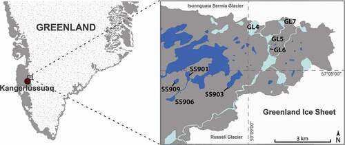
The area around Kangerlussuaq in west Greenland has warmed in recent decades, with 5.1°C and 1.9°C increases in spring and summer, respectively, during the period from 1981 to 2011 (Hanna et al. 2012). Because of this rapid warming, and the fact that GrIS meltwater flux is highest in this region (Lewis and Smith 2009), lakes near the ice-sheet margin in this area are ideal for addressing our questions. Bedrock in this area is composed of granitic gneiss (Nielson 2010). Target lakes were located along the GrIS and were sampled during the summer of 2015 (Figure 1). Glacially fed lakes included GL4, GL5, GL6, and GL7. Of those, GL4 and GL7 are headwater lakes, with both feeding into lakes GL5 and GL6. Glacially fed lake sizes ranged from 0.05 km² to 0.44 km² (Table 1). Snow- and groundwater-fed lakes included SS901, SS903, SS906, and SS909. There is some surficial flow of water occasionally from lake SS906 to lake SS901. Snow- and groundwater-fed lake sizes ranged from 0.06 km² to 0.36 km². Lakes GL4, GL5, and GL6 were resampled in the summer of 2016 for Chl a and surface sediments.

Table 1. Lake characteristics and sampling information. The only samples collected in 2016 were Chl a for the three indicated GF lakes and surface sediments from GL6. Surface sediments were used for both diatom counts and Psenner extractions

Lake	Type	Area (km^2)	Location (Deg Min Sec N & W)	Anchored depth (m)	Years Sampled	Surface Sediment Collection Location
GL4	GF	0.44	67°09ʹ28”, 50°08ʹ44”	28	2015, 2016	Shore
GL5	GF	0.13	67°09ʹ03”, 50°07ʹ26”	17	2015, 2016	Basin
GL6	GF	0.05	67°08ʹ43”, 50°07ʹ29”	5.5	2015, 2016	Basin
GL7	GF	0.08	67°09ʹ33”, 50°06ʹ18”	Sampled from shore	2015	Shore
SS901	SF	0.12	67°07ʹ52”, 50°14ʹ03”	14	2015	Basin
SS903	SF	0.36	67°07ʹ45”, 50°10ʹ19”	21.5	2015	Basin
SS906	SF	0.09	67°07ʹ09”, 50°15ʹ20”	18	2015	Basin
SS909	SF	0.06	67°07ʹ42”, 50°14ʹ59”	15	2015	Basin

Figure 1. Map of study area, showing the locations of lakes relative to the Greenland Ice Sheet. Glacially fed (GF) lakes are indicated in light blue, and snow- and groundwater-fed (SF) lakes are dark blue

All SF lakes included in this study stratify during summer, with oxygen-profile data collected every summer since 2013 suggesting that SF lake hypolimnia remain oxygenated (data not shown). Epilimnion depths in our target SF lakes, excluding SS909, ranged from 5 m (SS906) to 11 m (SS903) in July 2013 (Saros et al. 2016). A weather station adjacent to SS903 indicated that average June temperatures at this location were 6.4°C and 7.6°C in 2013 and 2014, respectively, and July temperatures were 7.6°C and 9.0°C. We did not collect temperature and oxygen profile data to determine whether summer stratification and anoxia occur in the GF target lakes. In turbid GF alpine lakes of the Austrian Alps, stratification occurs because of the absorbance of solar radiation by glacier flour particulates at the lake surface (Peter and Sommaruga 2017). The surface temperatures of these stratified lakes can reach 16.65°C. These stratified lakes often mix following precipitation events, because of the intrusion of cold water into the lake surface, and are classified as discontinuous cold polymictic. If west Greenland GF lakes stratify, the relatively small amount of summer precipitation in this region suggests that precipitation-induced mixing events would not occur.

Water parameters

Chemical and physical water parameters were measured to determine differences between GF and SF lakes and to assess their relationship to diatom community structure from each lake type. Water temperature, conductivity, and pH were measured at the lake surface using a submersible HydroLab Datasonde 5A instrument. Turbidity was measured using a handheld turbidimeter (AquaFluor by Turner Designs). These parameters were measured from the deepest point of each lake, except for GL4, GL6, and GL7, which were measured near shore. Water clarity was determined using a Secchi disk deployed from a raft and averaging two consecutive depth measurements. Secchi depth was not collected from GL7 because of logistical constraints. In SF lakes, surface water was collected using a van Dorn bottle deployed from the side of a rubber raft. In GF lakes, water was either collected with a van Dorn bottle deployed from a raft or sampled near shore at 1 m depth in the case of GL4 and GL7.

Chl a was determined by filtering surface water through Whatman GF/F filters, which were stored frozen until analysis. Chl a was extracted from filters with 90 percent acetone, centrifuged, and quantified with a Varian Cary-50 Ultraviolet-Visible spectrophotometer (Agilent Technologies; APHA 2000). Chl a was collected from target lakes in the summer of 2015 and again for GL4, GL5, and GL6 in the summer of 2016. Values were averaged across years for those repeat samples. Total alkalinity was determined on unfiltered lake water by titration with 0.2N H₂SO₄ to pH 4.5 (American Public Health Association [APHA] 2000). Total alkalinity was not collected from SF lake SS909 because of logistical constraints. Water used for dissolved nutrients (NH₄⁺, NO₃⁻, and SRP) and DOC was filtered through prerinsed Whatman GF/F filters and stored in acid-washed bottles. Dissolved and total nutrient samples (TN and TP) were analyzed on a Lachat QuickChem 8500 analyzer. NH₄⁺, NO₃⁻, and SRP were analyzed with the phenate, cadmium reduction, and ascorbic acid methods, respectively (APHA 2000). NH₄⁺ and NO₃⁻ were added together as dissolved inorganic nitrogen (DIN). Unfiltered TN and TP samples were measured as NO₃⁻ or SRP following persulfate digestion (APHA 2000). DOC was measured using a Shimadzu TOC analyzer.

Sediment Psenner extractions

Sediment Fe hydroxide (Fe(OH)₃) and especially aluminum (Al) hydroxide (Al(OH)₃) adsorb P in lake water and sediments, and can control P availability to microbes (Kopáček et al. 2005; Norton et al. 2011). Thus, as one measure of P bioavailability, we performed stepwise extractions of P, Fe, and Al on the top 0–2 cm (0–3 cm for GL6) of lake sediments. Because of logistical constraints, GL4 and SS909 sediments were not collected for this analysis. This sequential analysis rapidly assesses sediment P, Fe, and Al concentrations. Ratios of these extractions can predict lake sediment P release in anoxic conditions (Kopáček et al. 2005). Lake sediments were collected with a gravity corer from the deepest point we were able to locate in each lake. Sediments were extruded and stored frozen in Whirl-pak bags until analysis. Following a modified method of Psenner, Pucsko, and Sager (1984), four sediment extractions were performed: (1) 0.5 NH₄Cl (in lieu of DI water; Tessier, Campbell, and Bisson 1979) extracts loose and readily available P, Fe, and Al from sediment porewater; (2) 0.11 M Na₂S₂O₄ buffered with 0.11 M NaHCO₃ (BD) collects reducible species (particularly Fe^III oxyhydroxides) and associated P; (3) 0.1 M NaOH collects P associated with Al(OH)₃ and organic material; and (4) 0.5 M HCl extracts P, Fe, and Al associated with mineral material such as calcite and apatite (Kopáček et al. 2005). Following incubation on a shaker with each extract solution, samples were centrifuged for fifteen minutes at 3,000 rpm to separate the extract from the sediment. After the extract was collected, the centrifugation step was immediately repeated with fresh extract solution. Supernatants from each extraction step were analyzed for P, Fe, and Al by inductively coupled plasma optical emission spectrometry (ICP-OES; Thermo Electron iCap 6300).

The potential for P release from lake sediments was evaluated using Al:Fe_{NH4Cl+BD+NaOH} (Al:Fe) and Al_NaOH:P_NH4Cl+BD (Al:P) ratios. Briefly, if Al:Fe is below 3 and Al:P is below 25, then P is predicted to be released from lake sediments in anoxic conditions. If either of these ratios is greater than these thresholds, P release from lake sediments is likely minimal (Kopáček et al. 2005).

The organic content of sediment (percent organic matter, or %OM) was determined using loss on ignition (Heiri, Lotter, and Lemcke 2001). Briefly, wet sediment was weighed, dried at 100°C for sixteen hours, and reweighed to determine water content. The dried sediment was heated in a muffle furnace at 550°C for four hours to combust all organic material. Finally, the combusted sediment was reweighed to determine %OM.

Extracellular enzyme activities

To assess microbial demand and acquisition efforts for C, N, and P, we measured microbial extracellular enzyme activities (EEAs) as described in Burpee et al. (2016). Briefly, whole water samples were collected from lake epilimnia with a van Dorn bottle or by hand in acid-washed bottles. Samples were stored unfiltered and frozen (−20°C) until analysis. The EEA samples were analyzed on a Thermo Electron Corporation Fluoroskan Ascent FL fluorescence spectrophotometer following the methods of Sinsabaugh and Foreman (2001) and Findlay et al. (2003), and the optimization procedures of German et al. (2011). Because GF lakes had low EEAs, assays were run for forty-eight hours. The four enzymes selected for the assay together approximate microbial demand for macronutrients C, N, and P; these include β-1,4-glucosidase (BG), β-1,4-N-acetylglucosaminidase (NAG), leucine aminopeptidase (LAP), and phosphatase (AP). Respectively, these enzymes were measured using the fluorescent-labeled substrates 4-MUB-β-D-glucoside, 4-MUB-N-acetyl-β-D-glucosaminide, L-Leucine-7-AMC, and 4-MUB-phosphate. While EEAs of individual enzymes estimate total microbial demand for the corresponding nutrient, enzyme ratios BG:NAG+LAP and BG:AP estimate microbial investment in C-acquisition efforts with respect to N and P (Sinsabaugh, Hill, and Shah 2009; Sinsabaugh et al. 2008).

Diatom community analysis

Diatom assemblages were enumerated from lake-surface sediments. Single lake-surface sediment samples (0–1 cm) were collected with a gravity corer in 2015 from each lake except for GL5 and GL6, which were collected in 2016. Lake SS909 sediments were not collected because of logistical constraints. Surface sediments for two glacial lakes, GL4 and GL7, were collected near shore from a depth of 1 m, using a trowel and being careful to minimize disturbance. No obvious microbial mats were present in the littoral zone that could have altered the diatom community structure collected in these areas. Sediments were treated with 10 percent HCl, followed by 30 percent H₂O₂, which removed carbonate and organic material, respectively. Diatom slides were prepared following Battarbee (1986). Diatoms were counted with an Olympus BX51 microscope under 1,000x magnification using oil immersion. A minimum of 300 diatom valves were counted and identified from each slide according to Krammer and Lange-Bertalot (1986–1991) and Spaulding, Lubinski, and Potapova (2010).

Statistical analyses

Differences in physical and chemical factors between GF and SF lakes were evaluated using one-way analysis of variance (ANOVA). Because water chemistry and physical parameters did not meet assumptions of normality, these were also evaluated using nonparametric Kruskal-Wallis rank sum tests, which were in agreement with ANOVA tests at a significance level of p = 0.05. Thus, ANOVA results are reported. Lake sediment extraction data were log₁₀ transformed to meet assumptions of normality. Principal component analyses (PCAs) were conducted to determine dominant environmental trends across lake types. Constrained correspondence analysis (CCA) was used to examine species distribution trends across sites and environmental variables. The analysis included the relative abundance values for the most dominant taxa (>5% relative abundance in a sample lake). TP, DIN, DOC, turbidity, and conductivity were log₁₀ transformed and evaluated as explanatory environmental variables. To determine species richness across sample lakes, rarefaction analysis was conducted using a sample size of 300 individuals. All statistical analyses and plots were produced using R (version 3.3.2). ANOVAs were completed using the car package (version 2.1-4; Fox and Weisberg 2011), and rarefaction analysis, PCA, and CCA were conducted using the vegan package (version 2.4-2; Oksanen et al. 2017). Boxplots were made using ggplot2 (version 2.2.1; Wickham 2009).

Results

Water quality

Water chemistry was distinct between GF and SF lakes: TP concentrations were six times greater in GF lakes compared to SF lakes (18 versus 3 μg L⁻¹, p < 0.01, n = 8; Figure 2A), although SRP was below detection (<2 μg L⁻¹ PO₄⁻³-P) in all lakes. DOC concentrations were greater in SF lakes than in GF lakes (7 versus <1 mg L⁻¹, p = < 0.01, n = 8; Figure 2G), as were TN concentrations (367 versus 63 μg L⁻¹, p < 0.01, n = 8; Figure 2C). DIN concentrations were higher in GF lakes, but not significantly so (9 μg L⁻¹ for SF lakes, 20 μg L⁻¹ for GF lakes, p = 0.10, n = 8; Figure 2E). Both NO₃⁻ and NH₄⁺, which make up the bulk of the DIN pool (Bergström 2010), were not significantly different between lake types when considered individually.

Figure 2. Physical and chemical properties of glacially fed (GF) and snow- and groundwater-fed (SF) lakes. Significant differences are indicated by *** (p < 0.001), ** (p = 0.001–0.01), or * (p = 0.01–0.05)

Glacially fed lakes along the GrIS were much more turbid than SF lakes (30.8 versus 1.8 nephelometric turbidity units [NFUs], p < 0.01, n = 8; Figure 2B), and water clarity, measured by Secchi disk depth, was very low in GF compared to SF lakes (0.2 versus 7.7 m, p < 0.01, n = 7; Figure 2D). Conductivity (n = 8) and total alkalinity (n = 7) were lower in GF lakes (24 μS cm⁻¹ and 4 mg L⁻¹, respectively) compared to SF lakes (107 μS cm⁻¹ and 46 mg L⁻¹, p values = 0.03 and 0.02; Figure 2H). However, lake water pH was not significantly different between lake types (6.5 for GF lakes, 5.9 for SF lakes, p = 0.18, n = 8). Average surface water temperature was similar across GF and SF lakes (8.4°C and 10.6°C, respectively, p = 0.39, n = 8; Figure 2F).

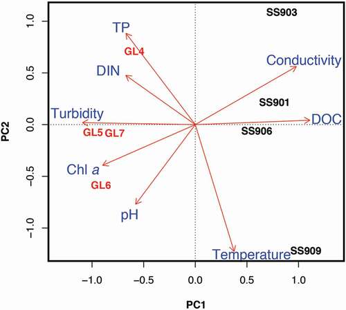
Principal component analyses of axes 1 and 2 explained 78 percent of the variance in lake features (Figure 3). Both GF and SF lakes separated along the first axis, which closely tracked turbidity (PC1 score −0.94) and DOC concentration (PC1 score 0.96) and explained 55 percent of the variation. Conductivity also tracked the first axis (PC1 score 0.84) with higher values in SF lakes. Although DIN was not significantly different between GF and SF lakes, PCA suggested that higher concentrations are associated with GF lakes (PC1 score −0.58). The second axis explained 23 percent of measured water-quality variation. Temperature and TP were oriented along the second axis (PC2 scores −0.85 and 0.61). SF lakes exhibited the most separation along the second axis, compared to GF lakes.

Figure 3. Principal component analysis (PCA) plot of physical and chemical properties of glacially fed (GF) and snow- and groundwater-fed (SF) lakes. GF lakes are labeled in red, SF lakes in black, and environmental variables in blue

Lake sediments

Differences in P chemistry between lake types were variable (n = 6): total extractable P (P_TE) was similar between GF and SF lakes (16.4 and 13.7 μmol g⁻¹ dry sediment, p = 0.25; Figure 4O), and the labile fraction of P_TE (P_NH4CL) was low across GF and SF lake sediments (<0.1 versus 0.1 μmol g⁻¹ dry sediment, p = 0.01; Figure 4K). However, other fractions of sediment P were distinct between GF and SF lakes. Fe^III oxyhydride-associated P (P_BD) was greater in SF compared to GF lakes (2.9 versus 0.3 μmol g⁻¹ dry sediment, p < 0.01; Figure 4L). Phosphorus associated with amorphous Al(OH)₃ and organic material (P_NaOH) was also greater in SF lakes compared with GF lakes (6.9 versus 2.0 μmol g⁻¹ dry sediment, p = 0.02; Figure 4M). In contrast, mineral-bound P (P_HCl) was roughly four times higher in GF lakes than SF lakes (14.1 versus 3.8 μmol g⁻¹ dry sediment, p < 0.01; Figure 4N).

Figure 4. Sequential sediment extractions for aluminum (Al; A–E), iron (Fe; F–J), and phosphorus (P; K–O) from glacially fed (GF) and snow- and groundwater-fed (SF) lake sediments. Significant differences are indicated by *** (p < 0.001), ** (p = 0.001–0.01), or * (p = 0.01–0.05)

Aluminum and Fe sediment chemistry differed between lake types (n = 6). Glacially fed lake sediments contained more total extractable Al (Al_TE) than SF lake sediments (127.4 versus 31.3 μmol g⁻¹ dry sediment, p < 0.01; Figure 4E). Porewater Al (Al_NH4Cl) concentrations were both low (<1 μmol g⁻¹ dry sediment; Figure 4A) and did not differ between lake types (p = 0.60). Further, Al_BD was similarly low and did not differ between lake types (1.1 and 1.3 μmol g⁻¹ dry sediment in SF and GF lakes, respectively, p = 0.60; Figure 4B). In contrast, amorphous Al (Al_NaOH) was nearly three times higher in GF lakes than in SF lakes (43.8 and 15.2 μmol g⁻¹ dry sediment, p = 0.01; Figure 4C). Mineral-associated Al (Al_HCl) was five times higher in GF lakes compared to SF lakes (82.2 and 14.9 μmol g⁻¹ dry sediment, respectively, p < 0.01; Figure 4D).

SF lake sediments contained more total extractable Fe (Fe_TE) than GF lake sediments (245.4 versus 112.8 μmol g⁻¹ dry sediment, p = 0.03; Figure 4J). Both lake types had low porewater Fe (Fe_NH4Cl; <1 μmol g⁻¹ dry sediment, p = 0.01; Figure 4F). Glacially fed lake sediments had greater concentrations of Fe^III oxyhydrides (Fe_BD) compared to SF lake sediments (158.9 versus 26.7 μmol g⁻¹ dry sediment, p < 0.01; Figure 4G). Fe_NaOH concentrations were not different between lake types (p = 0.31; Figure 4H). Mineral-extractable Fe (Fe_HCl) was similar between lake sediments (70.6 and 77.2 μmol g⁻¹ dry sediment for SF and GF lakes, respectively, p = 0.67; Figure 4I).

Both Al:Fe and Al:P, indices that estimate the potential for P release from lake sediments under anoxic conditions (Kopáček et al. 2005), were both higher in GF lakes compared to SF lakes (n = 6): 1.5 and 147.5 in GF lakes, respectively, and 0.1 and 5.4 in SF lakes (p values <0.01; Figure 5). Because P release is predicted if Al:Fe is below 3 and Al:P is below 25, these values indicate that P is more strongly bound to lake sediments in GF lakes, whereas P release from SF lake sediments under anoxia is probable. Lake sediments from SF lakes contained more organic matter (OM) than GF lake sediments (12.0 versus 1.7% OM, p < 0.01).

Figure 5. Ratios of glacially fed (GF) and snow- and groundwater-fed (SF) lake sediment extractions. Phosphorus (P) release from sediments during anoxia is predicted if aluminum to iron (Al:Fe_{NH4Cl+BD+NaOH}) is below 3 and if aluminum to phosphorus (Al_NaOH:P_NH4Cl+BD) is below 25

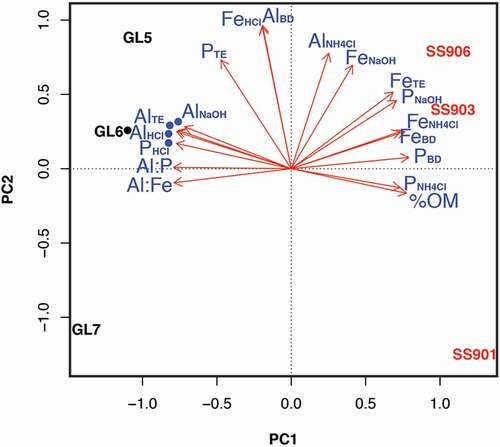
Principal component analyses of axes 1 and 2 explained 91 percent of the variation associated with lake sediment Al, Fe, and P speciation. The PCA demonstrated a separation of SF and GF lake sediments along the first axis, which tracked an organic (%OM, PC1 score 0.71) to mineral gradient (P_HCl and Al_HCl, PC1 scores −0.71 and −0.70; Figure 6). Generally, Al and Fe also separated out across the first axis, with Al extractions associated with GF lakes and Fe extractions associated with SF lakes. Porewater Al (Al_NH4Cl) and mineral Fe (Fe_HCl) were the exceptions to this pattern. Fe_HCl, Al_NH4Cl, and Al associated with reducible metal species (Al_BD) tracked PCA of axis 2 (PC2 scores −0.65, 0.53, and 0.65, respectively), which separated both GF and SF lakes. While most P fractions were associated with SF lakes, P_HCl was associated with GF lakes. The ratios Al:Fe and Al:P were strongly associated with GF lakes as well.

Figure 6. Principal component analysis (PCA) plot of sequential extractions from glacially fed (GF) and snow- and groundwater-fed (SF) lake sediments. GF lakes are labeled in red, SF lakes in black, and extraction variables in blue. Percent organic matter = %OM

Biological metrics

Phosphatase activity, indicating microbial P demand, was similar between lake types (0.19 versus 0.17 μmol mL⁻¹ h⁻¹ in SF and GF lakes, respectively, p = 0.60, n = 8; Table 2). However, other enzyme activities were different between lake types. Both BG and NAG+LAP activities, indicating microbial C and N demand, respectively, were higher in SF lakes (0.10 and 0.23 μmol mL⁻¹ h⁻¹, respectively), and were low enough in GF lakes to reach limits of detection (both <0.01 μmol mL⁻¹ h⁻¹, p values = 0.03 and <0.01, n = 8). Both BG:AP and BG:NAG+LAP ratios, indicative of microbial investment in C acquisition relative to P and N, respectively, were higher in SF lakes (0.48 and 0.41) than in GF lakes (<0.01 and 0.05, p values < 0.01 and = 0.02, n = 8).

Table 2. Microbial extracellular enzyme activities (EEAs) of glacially fed (GF) and snow- and groundwater-fed (SF) lakes. EEA units are μmol mL⁻¹ h⁻¹. Significant differences (p ≤ 0.05) between lake types are indicated by an asterisk (*)

Lake Type	BG	NAG + LAP	AP	BG:(NAG + LAP)	BG:AP
GF	<0.01*	<0.01*	0.17	0.05*	<0.01*
SF	0.01	0.23	0.19	0.41	0.48

Glacially fed lakes contained higher water column Chl a concentrations (1.7 versus 1.0 μg L⁻¹ in SF lakes, p = 0.03, n = 8), possibly indicating greater planktonic algal biomass (Figure 7A). Although GF lakes had slightly lower diatom species richness, it was not significantly different between GF and SF lakes (22.1 and 33.0, respectively, p = 0.28, n = 7; Figure 7B).

Figure 7. Chlorophyll a (Chl a) as a measure of algal biomass (a) and average diatom species richness, determined by rarefaction analysis (b). Significant differences are indicated by *** (p < 0.001), ** (p = 0.001–0.01), or * (p = 0.01–0.05)

Surface sediments (n = 7) demonstrated that both lake types were dominated by benthic diatom taxa, mostly belonging to the Achnanthidium or Psammothidium genera. Abundant (>5% relative abundance) planktonic or tychoplanktonic taxa included Lindavia ocellata, Discostella stelligera, Aulacoseira perglabra and Fragilaria vaucheriae, Fragilaria tenera, Staurosira construens, Staurosira construens var. venter, and Staurosirella pinnata. Lindavia ocellata was only present in SS901 and SS906, which are hydrologically connected (3.5 and 8.1 percent relative abundance, respectively), while D. stelligera was present in all SF lakes (11 percent mean relative abundance) and in GL5 and GL6, also hydrologically connected (14 percent mean relative abundance). Achnanthes species were the most dominant in SS903 (all Achnanthes species, representing 69 percent relative abundance). Achnanthidium minutissimum was also common in GF lakes (17 percent mean relative abundance). All Psammothidium species (Psammothidium chlidanos, Psammothidium scoticum, and Psammothidium subatomoides) were found solely in GF lakes. For GF lakes, mean percent relative abundances for P. chlidanos and P. scoticum were 10 and 23, respectively. Psammothidium subatomoides was only found in the littoral sediments of GL4 (19 percent relative abundance). Fragilaria vaucheriae and F. tenera were only present in GF lakes (7.0 and 5.4 mean percent relative abundance, respectively). Staurisirella pinnata was observed mostly in SF lakes (9 percent mean relative abundance), although it was also present in GL5 and GL6 (4 percent mean relative abundance). Staurosira construens was observed mostly in SF lakes (21 percent mean relative abundance), although it was also present in GL5 (0.8 percent relative abundance). Staurosira construens var. venter was only present in GL5 and GL6 (10.7 and 1.1percent relative abundance, respectively).

CCA axes 1 and 2 explained 65 percent of the overall variation (and 69 percent of the constrained variation) of abundant diatom species distributions across lakes (Figure 8). When CCA axis 3 was included, the overall and constrained variation explained increased to 82 percent and 87 percent, respectively. Sites were distributed across a DOC (0.90 CCA1 biplot score) versus TP and turbidity gradient (−0.89 and −0.94 CCA1 scores, respectively). Discostella stelligera was associated more with the second axis than the first (CCA1 score = 0.20 versus CCA2 score = −0.80).

Figure 8. Canonical correspondence analysis (CCA) plot of diatom species distribution (right panel) across glacially fed (GF) and snow- and groundwater-fed (SF) lakes (left panel), determined by nutrient and turbidity variables (middle panel). Turb = turbidity and Cond = conductivity

Discussion

We found that lakes fed by GrIS meltwater have distinct physical, chemical, and biological characteristics. Compared to SF lakes, differences included higher concentrations of TP and possibly DIN in GF lake water, although the difference in DIN was not significant. While the different sampling locations (pelagic versus littoral) in GF lakes may have affected our results, we note that the chemistry across GF samples was more similar than that in GF compared to SF lakes. These findings support our first hypothesis that GF lakes would have higher concentrations of phosphorus and DIN compared to SF lakes, although we could not assess P bioavailability from TP measurement alone. Conversely, SF lakes had higher concentrations of DOC and TN than GF lakes. DOC and TN tightly covary in SF lakes surrounding Kangerlussuaq (Burpee et al. 2016). Therefore, the high TN concentrations in SF lakes are likely because of large DOC pools that contain organic N. We also determined that physical environments of GF lakes, measured by turbidity and water clarity, were different than those of SF lakes, while surface water temperatures were similar.

The enhanced P concentrations found in GF lakes in Greenland differ from patterns in GF alpine lakes in North America, which have higher NO₃-N than SF lakes but similarly low P (Saros et al. 2010; Slemmons and Saros 2012; Williams et al. 2007). Bedrock underlying the GrIS at our study location consists of P-containing minerals, such as fluorapatite (Hawkings et al. 2016; Porder and Ramachandran 2013). Further, the subglacial environments of continental ice sheets such as the GrIS are biogeochemically reactive and have high weathering rates (Hawkings et al. 2016; Wadham et al. 2010). High TP concentrations are present in other Arctic and alpine glacier meltwaters in Svalbard, Sweden, France, and Pakistan (Hodson, Mumford, and Lister 2004). In contrast, low TP in North American GF alpine lakes could be attributable to different bedrock types and lower subglacial weathering rates. This region has slow weathering bedrock, for instance (Saros et al. 2005).

Whether the source of nitrate in alpine glacier meltwater in the North American Rocky Mountains is attributable to subglacial microbial and weathering processes or atmospheric deposition (i.e., the alpine distillery effect; Daly and Wania 2005) remains unclear (Saros et al. 2010; Williams et al. 2007). Principal component analyses associated DIN with GF lakes along the GrIS, and GF lakes had a higher mean concentration of DIN than SF lakes, although the difference was not statistically significant. Elevated DIN in GF lakes could be attributable to weathered minerogenic sources (Holloway and Dahlgren 2002) or to increases in anthropogenic N deposition in Greenland since the mid-nineteenth century (Hastings, Jarvis, and Steig 2009). Regardless of the sources, we found evidence that, similar to GF alpine lakes, glacial meltwaters to these Arctic lakes alter the nutrient chemistry compared to nearby SF lakes.

Although these GF lakes have higher concentrations of TP and higher algal biomass than SF lakes, sediment chemistry analyses raise questions about the bioavailability of this P to microbial communities. While GF and SF lake sediments contained similar amounts of P_TE, most GF sediment P was in the mineral phase, whereas SF lakes had higher P content in more labile phases. Since the same suspended glacial flour that contributes to water turbidity settles to the bottom and constitutes GF lake sediments, it is likely that the P content of sediments and whole water samples are similar in GF lakes. Thus, the high TP measured in GF lake water is likely due primarily to mineral-associated P. The fact that SRP and DOC are both extremely low in GF meltwater minimizes these as potential sources contributing to TP. Our findings are consistent with other work that reports that glacial meltwaters in Svalbard, France, and Pakistan contain high TP, but low algal-available P (P_NaOH; Hodson, Mumford, and Lister 2004).

Higher Al content in GF lake sediments could further modify P availability to microbes. For instance, Al(OH)₃ can adsorb to P, thus preventing its release from the sediment into the water column (Kopáček et al. 2005; Kopáček et al. 2000). Norton et al. (2011) demonstrated that during the course of 16.6 thousand years following deglaciation, Al species introduced into a northeast American lake from developing catchment soils sequestered P from the water column. Diatom community changes tracked this declining P. Thus, high Al:Fe and Al:P ratios provide further evidence that GF lakes have less potential to release adsorbed P from glacial flour material (Kopáček et al. 2005). Last, our EEA results suggest high microbial demand for P relative to C and N, implying that P is biologically scarce in GF lakes; however, these results should be interpreted with caution because the C and N enzyme activities were below detection. These low activities may reflect actual microbial demand, or possibly enzyme interference by adsorption to fine-grained mineral particles (Tietjen and Wetzel 2003). Together, these data suggest that while GF lakes have high TP concentrations, the bioavailablility of this pool may be low.

Some GF lakes in alpine regions are clear, not turbid; this is the case in many GF lakes of the central North American Rocky Mountains (Saros et al. 2010; Slemmons and Saros 2012). In that area, high water clarity in alpine GF lakes is likely because of glacial flour settling and becoming entrained in lake inlet streams (Saros et al. 2010), relatively reduced rates of weathering activity, and reduced amounts of glacier flour produced by comparatively smaller alpine glaciers. In other areas, turbidity is likely an important driver of lake ecology in GF lakes; decreasing turbidity throughout a 400-year alpine lake-sediment pigment record was one of the factors implicated in driving increased primary production (Vinebrooke et al. 2010). In contrast, Kammerlander et al. (2016) demonstrated increased abundance and richness of algae and ciliates in an alpine GF turbid lake, compared to a clear lake. Our own evidence suggests that in addition to nutrient subsidies, lake turbidity is an important factor that corresponds to diatom species distribution across target lakes along the GrIS.

The similarity of surface temperatures between GF and SF lakes in Greenland is also consistent with patterns in some clear GF and SF alpine lakes (Slemmons and Saros 2012). We were unable to collect thermal profile data from the GF lakes studied here, hence it remains unclear whether vertical temperature gradients differ between GF and SF lakes in this region. In other regions, such as the Austrian Alps, the turbidity of GF lakes alters thermal stratification patterns compared to those of SF lakes, with turbid GF alpine lakes being polymictic (Peter and Sommaruga 2017; Sommaruga 2015). The surface temperatures of the target Greenland GF lakes were lower than the alpine lakes observed by Peter and Sommaruga (2017), however, which can reach temperatures as high as 16.65°C. The average surface temperature of the GF lakes included in this study (8.4°C) suggests that stratification was not occurring at the time of observation.

Lakes surrounding Kangerlussuaq are mostly closed basins in which evaporative concentration controls lake-water chemistry (Anderson et al. 2001). Thus, higher conductivity in SF lakes results from longer residence times and subsequently higher concentrations of ions due to evaporative concentration. Glacially fed lakes have shorter residence times than SF lakes, owing to greater surface outflows.

Higher water column algal biomass in Greenland GF lakes is consistent with patterns in other clear and turbid alpine GF lakes (Kammerlander et al. 2016; Slemmons and Saros 2012; Slemmons et al. 2015). This elevated planktonic algal biomass may be driven by P inputs, as even small amounts of labile P associated with mineral glacial flour can be biologically significant (Hodson, Mumford, and Lister 2004). Additionally, elevated DIN concentrations in GF and SF alpine lakes have a positive effect on algal biomass (Das et al. 2005; Slemmons and Saros 2012; Slemmons et al. 2015), and could be responsible for the high water column Chl a in these GrIS-fed lakes. Finally, higher Chl a concentrations that occur in some GF turbid lakes may be driven by altered light availability (Kammerlander et al. 2016), which can lead to an increase in low-light adapted algae, such as cryptophytes (Gervais 1997), which were not counted in this study. Furthermore, some algae can adapt to lower light intensities by increasing Chl a content per cell (Jøsrgensen 1969). It must therefore be noted that although we use Chl a as a proxy for algal biomass, the proportional relationship between Chl a and biomass could differ between turbid GF and clear SF lakes.

Algal biomass is often negatively correlated to species richness (Interlandi and Kilham 2001), but our hypothesis that GF lakes would have reduced species richness was not supported, despite this being observed in clear, N-subsidized alpine GF lakes (Saros et al. 2010). Species richness in Greenland GF lakes may be even higher than our reported value, which included littoral samples from GL4 and GL7. Some turbid GF lakes exhibit greater protistan (ciliates and algae) species richness, likely owing to photoprotection and expanded resource niches (Kammerlander et al. 2016). Thus, the reduced species richness expected of nutrient-subsidized GF lake diatom communities (in accordance with resource competition theory; Interlandi and Kilham 2001) may be offset by lake turbidity, which constrains light availability and reduces exposure to harmful light, thereby offsetting reductions in richness from nutrient enrichment.

Turbidity was the most important environmental variable that tracked diatom species distributions across the study lakes, closely followed by DOC and TP. Lakes that had similar landscape position and hydrological connectivity had more similar diatom communities. This was true for GL5 and GL6, and SS901 and SS906. Although GL4 and GL7 were not hydrologically connected, they had similar diatom communities that could reflect direct adjacency to the GrIS. Benthic diatom taxa were abundant in both lake types, suggesting that benthic diatom abundance was not caused by differences in lake-water chemistry. Benthic diatom dominance was unexpected in GF lakes because of high turbidity and low water clarity. The high proportion of GF lake benthic diatom abundance may be because of increased diatom productivity in the shallow littoral zones and relatively less productivity in the turbid water columns of GF lakes. Benthic diatoms, including a high abundance of Psammothidium and Achnanthidium species, exist in supraglacial cryoconite holes on the surface of Antarctic and Arctic glaciers (Stanish et al. 2013; Vinšová et al. 2015; Yallop and Anesio 2010). Thus, diatom assemblages of GF lakes along the GrIS could be dominated by supraglacial communities arriving via meltwater. The fact that the surface sediments were collected from littoral zones for two out of the four GF lakes (GL4 and GL7) could also inflate the observed benthic diatom abundance. Both GL4 and GL7 clustered together in our CCA (Figure 8), suggesting similar environments from which the surface sediments were collected. Further, the sample size of GF lakes (n = 4) is small in this study, and may not represent typical GrIS-fed systems. These considerations are important to consider while interpreting our algal community data. Nevertheless, even GF lake surface sediments collected from greater depths (GL5 and GL6) contained high proportions of benthic diatom species, such as A. minutissimum, S. construens var. venter, and F. vaucheriae.

Diatom communities were different between GF and SF lakes, and while some species were abundant in both lake types (D. stelligera and A. minutissimum), most were abundant in either one or the other. The presence of F. tenera only in GF lakes is consistent with nutrient-enriched alpine GF lakes (Kammerlander et al. 2016; Slemmons et al. 2015), and northeast Greenland Bunny Lake (Slemmons et al. 2016), and is associated with N enrichment (Das et al. 2005; Sheibley et al. 2014). In contrast, F. tenera was present in nonglacial central and northeastern Greenland coastal lakes, although lake nutrients were not evaluated in this study (Cremer and Wagner 2004). Paleolimnological evidence from North American alpine lakes suggests that, compared to a SF lake, the GF Jasper Lake had earlier dominance by key diatom species with moderate N requirements, such as Asterionella formosa and Fragilaria crotonensis (Slemmons et al. 2015). In east Greenland, the sedimentary diatom profile from Bunny Lake, fed by the Renland Ice Cap, revealed an increase in the relative abundances of taxa such as F. crotonensis, Fragilaria tenera, and Tabellaria flocculosa as glacial meltwater influx increased about 1,000 years ago (Slemmons et al. 2016). These diatom community shifts were attributed to changes in lake physical and nutrient characteristics induced by meltwater inputs, but contemporary data on these lake features were not available. Further, Discostella stelligera can be indicative of DIN enrichment (Köster and Pienitz 2006; Perren, Axford, and Kaufman 2017), and its high relative abundance in Greenland GF lakes is also consistent with that found in alpine GF lakes (Slemmons et al. 2015). It is possible that D. stelligera is also in GL4 and GL7, but our sediment samples were from the littoral zones of these lakes, and would underrepresent planktonic taxa if they are there. Together, these data suggest that the moderately elevated DIN in GF lakes is an important resource subsidy.

In conclusion, we show that GF lakes along the GrIS have their own distinct physical, chemical, and biological features compared to SF lakes in the area. Although high turbidity, elevated TP, and moderate DIN appear to be important drivers of GF lake algal ecology, our work suggests that Al contributions to GrIS-associated lakes have important interactions with P and likely reduce its bioavailability in GF lakes. Our results contribute to the growing body of literature that reveals the spatial variability in the effects of glacial meltwaters on Arctic and alpine lakes worldwide. In turn, lakes play key roles in biogeochemical cycling in these regions. Their growing numbers with glacial recession underscore their increasing importance in regional responses to global changes.

Acknowledgments

We thank Rachel Fowler, Robert Northington, Kristin Strock, Max Egener, Andrea Nurse, Helen Schlimm, Carl Tugend, and Kate Warner for field assistance, and the CPS staff for support in the field. We additionally thank Robert Northington for nutrient analysis, Stephen Norton for assistance with Psenner methods, and Johanna Cairns for assistance in figure rendering. Discussions with Ruben Sommaruga greatly improved data interpretation.

Additional information

Funding

Funding for this project was provided by the U.S. National Science Foundation (Grants no. 1203434 and 1144423).

References

- American Public Health Association (APHA). 2000. Standard methods for the examination of Water and Wastewater, 20th ed. Washington, D.C: American Public Health Association, American Water Works Association, Water Environment Federation.
- Anderson, N. J., R. Harriman, D. B. Ryves, and S. T. Patrick. 2001. Dominant factors controlling variability in the ionic composition of West Greenland lakes. Arctic, Antarctic, and Alpine Research 33 (4):1–15. doi:https://doi.org/10.2307/1552551.
- Anderson, N. J., J. E. Saros, J. E. Bullard, S. M. Cahoon, S. McGowan, E. A. Bagshaw, C. D. Barry, R. Bindler, B. T. Burpee, J. L. Carrivick, et al. 2017. The Arctic in the twenty-first century: Changing biogeochemical linkages across a paraglacial landscape of Greenland. Bioscience 67 (2):118–33.
- Battarbee, R. W. 1986. Diatom analysis. In Handbook of Holocene palaeoecology and palaeohydrology, ed. B. E. Berglund, 527–70. New York: Wiley-Interscience.
- Bergström, A. K. 2010. The use of TN:TP and DIN:TP ratios as indicators for phytoplankton nutrient limitation in oligotrophic lakes affected by N deposition. Aquatic Sciences 72:277–81. doi:https://doi.org/10.1007/s00027-010-0132-0.
- Bhatia, M. P., E. B. Kujawinski, S. B. Das, C. F. Breier, P. B. Henderson, and M. A. Charette. 2013. Greenland meltwater as a significant and potentially bioavailable source of iron to the ocean. Nature Geoscience 6 (4):274–78. doi:https://doi.org/10.1038/ngeo1746.
- Burpee, B., J. E. Saros, R. M. Northington, and K. S. Simon. 2016. Microbial nutrient limitation in Arctic lakes in a permafrost landscape of southwest Greenland. Biogeosciences 13 (2):365–74. doi:https://doi.org/10.5194/bg-13-365-2016.
- Carrivick, J. L., and F. S. Tweed. 2013. Proglacial lakes: Character, behavior and geological importance. Quaternary Science Reviews 78:34–52. doi:https://doi.org/10.1016/j.quascirev.2013.07.028.
- Cole, J. J., M. L. Pace, S. R. Carpenter, and J. F. Kitchell. 2000. Persistence of net heterotrophy in lakes during nutrient addition and food web manipulations. Limnology and Oceanography 45 (8):1718–30. doi:https://doi.org/10.4319/lo.2000.45.8.1718.
- Cremer, H., and B. Wagner. 2004. Planktonic diatom communities in High Arctic lakes (Store Koldewey, Northeast Greenland). Canadian Journal of Botany 82 (12):1744–57. doi:https://doi.org/10.1139/b04-127.
- Daly, G. L., and F. Wania. 2005. Organic contaminants in mountains. Environmental Science & Technology 39 (2):385–98. doi:https://doi.org/10.1021/es048859u.
- Das, B., R. D. Vinebrooke, A. Sanchez-Azofeifa, B. Rivard, and A. P. Wolfe. 2005. Inferring sedimentary chlorophyll concentrations with reflectance spectroscopy: A novel approach to reconstructing historical changes in the trophic status of mountain lakes. Canadian Journal of Fisheries and Aquatic Sciences 62 (5):1067–78. doi:https://doi.org/10.1139/f05-016.
- Fegel, T. S., J. S. Baron, A. G. Fountain, G. F. Johnson, and E. K. Hall. 2016. The differing biogeochemical and microbial signatures of glaciers and rock glaciers. Journal of Geophysical Research: Biogeosciences 121:919–32.
- Findlay, S. E., R. L. Sinsabaugh, W. V. Sobczak, and M. Hoostal. 2003. Metabolic and structural response of hyporheic microbial communities to variations in supply of dissolved organic matter. Limnology and Oceanography 48 (4):1608–17. doi:https://doi.org/10.4319/lo.2003.48.4.1608.
- Fox, J., and S. Weisberg. 2011. An {R} companion to applied regression, 2nd ed. Thousand Oaks, CA: Sage.
- German, D. P., M. N. Weintraub, A. S. Grandy, C. L. Lauber, Z. L. Rinkes, and S. D. Allison. 2011. Optimization of hydrolytic and oxidative enzyme methods for ecosystem studies. Soil Biology and Biochemistry 43 (7):1387–97. doi:https://doi.org/10.1016/j.soilbio.2011.03.017.
- Gervais, F. 1997. Light-dependent growth, dark survival, and glucose uptake by cryptophytes isolated from a freshwater chemocline. Journal of Phycology 33 (1):18–25. doi:https://doi.org/10.1111/j.0022-3646.1997.00018.x.
- Granshaw, F. D., and A. G. Fountain. 2006. Glacier change (1958–1998) in the north Cascades national park complex, Washington, USA. Journal of Glaciology 52 (177):251–56. doi:https://doi.org/10.3189/172756506781828782.
- Hanna, E., P. Huybrechts, K. Steffen, J. Cappelen, R. Huff, C. Shuman, T. Irvine-Fynn, S. Wise, and M. Griffiths. 2008. Increased runoff from melt from the Greenland Ice Sheet: A response to global warming. Journal of Climate 21 (2):331–41. doi:https://doi.org/10.1175/2007JCLI1964.1.
- Hanna, E., S. H. Mernild, J. Cappelen, and K. Steffen. 2012. Recent warming in Greenland in a long-term instrumental (1881–2012) climatic context: I. Evaluation of surface air temperature records. Environmental Research Letters 7 (4):045404. doi:https://doi.org/10.1088/1748-9326/7/4/045404.
- Hastings, M. G., J. C. Jarvis, and E. J. Steig. 2009. Anthropogenic impacts on nitrogen isotopes of ice-core nitrate. Science 324 (5932):1288. doi:https://doi.org/10.1126/science.1170510.
- Hawkings, J., J. Wadham, M. Tranter, J. Telling, E. Bagshaw, A. Beaton, S. L. Simmons, D. Chandler, A. Tedstone, and P. Nienow. 2016. The Greenland Ice Sheet as a hot spot of phosphorus weathering and export in the Arctic. Global Biogeochemical Cycles 30:191–210. doi:https://doi.org/10.1002/2015GB005237.
- Hawkings, J. R., J. L. Wadham, M. Tranter, E. Lawson, A. Sole, T. Cowton, A. J. Tedstone, I. Bartholomew, P. Nienow, D. Chandler, et al. 2015. The effect of warming climate on nutrient and solute export from the Greenland Ice Sheet. Geochemical Perspectives Letters 1:94–104. doi:https://doi.org/10.7185/geochemlet.1510.
- Heiri, O., A. F. Lotter, and G. Lemcke. 2001. Loss on ignition as a method for estimating organic and carbonate content in sediments: Reproducibility and comparability of results. Journal of Paleolimnology 25 (1):101–10. doi:https://doi.org/10.1023/A:1008119611481.
- Hodson, A., P. Mumford, and D. Lister. 2004. Suspended sediment and phosphorus in proglacial rivers: Bioavailability and potential impacts upon the P status of ice: Marginal receiving waters. Hydrological Processes 18 (13):2409–22. doi:https://doi.org/10.1002/(ISSN)1099-1085.
- Holloway, J. M., and R. A. Dahlgren. 2002. Nitrogen in rock: Occurrences and biogeochemical implications. Global Biogeochemical Cycles 16 (4):1118. doi:https://doi.org/10.1029/2002GB001862.
- Interlandi, S. J., and S. S. Kilham. 2001. Limiting resources and the regulation of diversity in phytoplankton communities. Ecology 82 (5):1270–82. doi:https://doi.org/10.1890/0012-9658(2001)082[1270:LRATRO]2.0.CO;2.
- Jøsrgensen, E. G. 1969. The adaptation of plankton algae IV. Light adaptation in different algal species. Physiologia Plantarum 22 (6):1307–15. doi:https://doi.org/10.1111/j.1399-3054.1969.tb09121.x.
- Kammerlander, B., K. A. Koinig, E. Rott, R. Sommaruga, B. Tartarotti, F. Trattner, and B. Sonntag. 2016. Ciliate community structure and interactions within the planktonic food web in two alpine lakes of contrasting transparency. Freshwater Biology 61 (11):1950–65. doi:https://doi.org/10.1111/fwb.2016.61.issue-11.
- Knight, P. G., R. I. Waller, C. J. Patterson, A. P. Jones, and Z. P. Robinson. 2000. Glacier advance, ice-marginal lakes and routing of meltwater and sediment: Russell Glacier, Greenland. Journal of Glaciology 46 (154):423–26. doi:https://doi.org/10.3189/172756500781833160.
- Kopáček, J., J. Borovec, J. Hejzlar, K. U. Ulrich, S. A. Norton, and A. Amirbahman. 2005. Aluminum control of phosphorus sorption by lake sediments. Environmental Science & Technology 39 (22):8784–89. doi:https://doi.org/10.1021/es050916b.
- Kopáček, J., J. Hejzlar, J. Borovec, P. Porcal, and I. Kotorova. 2000. Phosphorus availability in an acidified watershed-lake ecosystem. Limnology and Oceanography 45 (1):212–25. doi:https://doi.org/10.4319/lo.2000.45.1.0212.
- Köster, D., and R. Pienitz. 2006. Seasonal diatom variability and paleolimnological inferences: A case study. Journal of Paleolimnology 35 (2):395–416. doi:https://doi.org/10.1007/s10933-005-1334-7.
- Krammer, K., and H. Lange-Bertalot. 1986–1991. Bacillariophyceae. In Sußwasserflora von Mitteleuropa, eds. H. Ettl, G. Gartner, J. Gerloff, H. Heynig, and D. Mollenhauer. Vols. 2 (1–4). Stuttgart/Jena: Gustav Fischer Verlag. (Freshwater flora of central Europe.).
- Lawson, E. C., J. L. Wadham, M. Tranter, M. Stibal, G. P. Lis, C. E. Butler, J. Laybourn-Parry, P. Nienow, D. Chandler, and P. Dewsbury. 2014. Greenland Ice Sheet exports labile organic carbon to the Arctic oceans. Biogeosciences 11 (14):4015–28. doi:https://doi.org/10.5194/bg-11-4015-2014.
- Lewis, S. M., and L. C. Smith. 2009. Hydrologic drainage of the Greenland Ice Sheet. Hydrological Processes 23 (14):2004–11. doi:https://doi.org/10.1002/hyp.v23:14.
- McClain, M. E., E. W. Boyer, C. L. Dent, S. E. Gergel, N. B. Grimm, P. M. Groffman, S. C. Hart, J. W. Harvey, C. A. Johnston, E. Mayorga, et al. 2003. Biogeochemical hot spots and hot moments at the interface of terrestrial and aquatic ecosystems. Ecosystems 6 (4):301–12. doi:https://doi.org/10.1007/s10021-003-0161-9.
- Nielsen, A. B., 2010. Present conditions in Greenland and the Kangerlussuaq area. Posiva Oy. Working Report no. 2010-07.
- Norton, S. A., R. H. Perry, J. E. Saros, G. L. Jacobson, I. J. Fernandez, J. Kopáček, T. A. Wilson, and M. D. SanClements. 2011. The controls on phosphorus availability in a Boreal lake ecosystem since deglaciation. Journal of Paleolimnology 46 (1):107–22. doi:https://doi.org/10.1007/s10933-011-9526-9.
- Oksanen, J., F. G. Blanchet, M. Friendly, R. Kindt, P. Legendre, D. McGlinn, P. R. Minchin, R. B. O’Hara, G. L. Simpson, P. Solymos, et al. 2017. vegan: Community ecology package. R Package Version 2.4-2.
- Pace, M. L., and J. J. Cole. 2000. Effects of whole-lake manipulations of nutrient loading and food web structure on planktonic respiration. Canadian Journal of Fisheries and Aquatic Sciences 57 (2):487–96. doi:https://doi.org/10.1139/f99-279.
- Perren, B. B., Y. Axford, and D. S. Kaufman. 2017. Alder, nitrogen, and lake ecology: Terrestrial-aquatic linkages in the postglacial history of lone spruce Pond, southwestern Alaska. PloS ONE 12 (1):0169106. doi:https://doi.org/10.1371/journal.pone.0169106.
- Peter, H., and R. Sommaruga. 2017. Alpine glacier-fed turbid lakes are discontinuous cold polymictic rather than dimictic. Inland Waters 7 (1):45–54. doi:https://doi.org/10.1080/20442041.2017.1294346.
- Porder, S., and S. Ramachandran. 2013. The phosphorus concentration of common rocks: A potential driver of ecosystem P status. Plant and Soil 367 (1–2):41–55. doi:https://doi.org/10.1007/s11104-012-1490-2.
- Psenner, R., R. Pucsko, and M. Sager. 1984. Die Fraktionierung organischer und anorganischer phosphorverbindungen von sedimenten: Versuch einer definition ökologisch wichtiger Frakionen. Archive Fur Hydrobiologie Supplement 70 (1):111–55.
- Saros, J. E., S. J. Interlandi, S. Doyle, T. J. Michel, and C. E. Williamson. 2005. Are the deep chlorophyll maxima in alpine lakes primarily induced by nutrient availability, not UV avoidance? Arctic, Antarctic, and Alpine Research 37 (4):557–63. doi:https://doi.org/10.1657/1523-0430(2005)037[0557:ATDCMI]2.0.CO;2.
- Saros, J. E., R. M. Northington, C. L. Osburn, B. T. Burpee, and N. J. Anderson. 2016. Thermal stratification in small arctic lakes of southwest Greenland affected by water transparency and epilimnetic temperatures. Limnology & Oceanography 61 (4):1530–42. doi:https://doi.org/10.1002/lno.10314.
- Saros, J. E., K. C. Rose, D. W. Clow, V. C. Stephens, A. B. Nurse, H. A. Arnett, J. R. Stone, C. E. Williamson, and A. P. Wolfe. 2010. Melting alpine glaciers enrich high-elevation lakes with reactive nitrogen. Environmental Science & Technology 44 (13):4891–96. doi:https://doi.org/10.1021/es100147j.
- Sheibley, R. W., M. Enache, P. W. Swarzenski, P. W. Moran, and J. R. Foreman. 2014. Nitrogen deposition effects on diatom communities in lakes from three national parks in Washington State. Water, Air, & Soil Pollution 225 (2):1857. doi:https://doi.org/10.1007/s11270-013-1857-x.
- Sinsabaugh, R. L., and C. M. Foreman. 2001. Activity profiles of bacterioplankton in a eutrophic river. Freshwater Biology (46):1239–49. doi:https://doi.org/10.1046/j.1365-2427.2001.00748.x.
- Sinsabaugh, R. L., B. H. Hill, and J. J. F. Shah. 2009. Ecoenzymatic stoichiometry of microbial organic nutrient acquisition in soil and sediment. Nature 462 (7274):795–98. doi:https://doi.org/10.1038/nature08632.
- Sinsabaugh, R. L., C. L. Lauber, M. N. Weintraub, B. Ahmed, S. D. Allison, C. Crenshaw, A. R. Contosta, D. Cusack, S. Frey, M. E. Gallo, et al. 2008. Stoichiometry of soil enzyme activity at global scale. Ecology Letters 11 (11):1252–64.
- Slemmons, K. E., A. Medford, B. L. Hall, J. R. Stone, S. McGowan, T. Lowell, M. Kelly, and J. E. Saros. 2016. Changes in glacial meltwater alter algal communities in lakes of Scoresby Sund, Renland, East Greenland throughout the holocene: Abrupt reorganizations began 1000 years before present. The Holocene 27 (7):929–40. doi:https://doi.org/10.1177/0959683616678468.
- Slemmons, K. E., and J. E. Saros. 2012. Implications of nitrogen-rich glacial meltwater for phytoplankton diversity and productivity in alpine lakes. Limnology and Oceanography 57 (6):1651–63. doi:https://doi.org/10.4319/lo.2012.57.6.1651.
- Slemmons, K. E., J. E. Saros, J. R. Stone, S. McGowan, C. T. Hess, and D. Cahl. 2015. Effects of glacier meltwater on the algal sedimentary record of an alpine lake in the central US Rocky Mountains throughout the late Holocene. Journal of Paleolimnology 53 (4):385–99. doi:https://doi.org/10.1007/s10933-015-9829-3.
- Smith, E. M., and Y. T. Prairie. 2004. Bacterial metabolism and growth efficiency in lakes: The importance of phosphorus availability. Limnology and Oceanography 49 (1):137–47. doi:https://doi.org/10.4319/lo.2004.49.1.0137.
- Sommaruga, R. 2015. When glaciers and ice sheets melt: Consequences for planktonic organisms. Journal of Plankton Research 37 (3):509–18. doi:https://doi.org/10.1093/plankt/fbv027.
- Spaulding, S. A., D. J. Lubinski, and M. Potapova, 2010: Diatoms of the United States. Accessed on March 11, 2017. http://westerndiatoms.colorado.edu.
- Stanish, L. F., E. A. Bagshaw, D. M. McKnight, A. G. Fountain, and M. Tranter. 2013. Environmental factors influencing diatom communities in Antarctic cryoconite holes. Environmental Research Letters 8 (4):045006. doi:https://doi.org/10.1088/1748-9326/8/4/045006.
- Tessier, A., P. Campbell, and M. Bisson. 1979. Sequential extraction procedure for the speciation of trace metals. Analytical Chemistry (51):844–51. doi:https://doi.org/10.1021/ac50043a017.
- Tietjen, T., and R. G. Wetzel. 2003. Extracellular enzyme-clay mineral complexes: Enzyme adsorption, alteration of enzyme activity, and protection from photodegradation. Aquatic Ecology 37 (4):331–39. doi:https://doi.org/10.1023/B:AECO.0000007044.52801.6b.
- van den Broeke, M., J. Bamber, J. Ettema, E. Rignot, E. Schrama, W. J. van de Berg, E. van Meijgaard, I. Velicogna, and B. Wouters. 2009. Partitioning recent Greenland mass loss. Science 326 (5955):984–86. doi:https://doi.org/10.1126/science.1178176.
- Vinebrooke, R. D., P. L. Thompson, W. Hobbs, B. H. Luckman, M. D. Graham, and A. P. Wolfe. 2010. Glacially mediated impacts of climate warming on alpine lakes of the Canadian Rocky Mountains. Verhandlungen Des Internationalen Verein Limnologie 30:1449–52.
- Vinšová, P., E. Pinseel, T. J. Kohler, B. van de Vijver, J. D. Žárský, J. Kavan, and K. Kopalová. 2015. Diatoms in cryoconite holes and adjacent proglacial freshwater sediments, Nordenskiöld glacier (Spitsbergen, High Arctic). Czech Polar Reports 5:112–33. doi:https://doi.org/10.5817/CPR2015-2-11.
- Wadham, J. L., M. Tranter, M. Skidmore, A. J. Hodson, J. Priscu, W. B. Lyons, M. Sharp, P. Wynn, and M. Jackson. 2010. Biogeochemical weathering under ice: Size matters. Global Biogeochemical Cycles 24 (3):GB3025. doi:https://doi.org/10.1029/2009GB003688.
- Wickham, H. 2009. ggplot2: Elegant Graphics for Data Analysis. New York: Springer-Verlag.
- Williams, J. J., A. Nurse, J. E. Saros, J. Riedel, and M. Beutel. 2016. Effects of glaciers on nutrient concentrations and phytoplankton in lakes within the Northern Cascades Mountains (USA). Biogeochemistry 131 (3):373–85. doi:https://doi.org/10.1007/s10533-016-0264-y.
- Williams, M. W., M. Knauf, R. Cory, N. Caine, and F. Liu. 2007. Nitrate content and potential microbial signature of rock glacier outflow, Colorado front range. Earth Surface Processes and Landforms 32 (7):1032–47. doi:https://doi.org/10.1002/(ISSN)1096-9837.
- Yallop, M. L., and A. M. Anesio. 2010. Benthic diatom flora in supraglacial habitats: A generic-level comparison. Annals of Glaciology 51 (56):15–22. doi:https://doi.org/10.3189/172756411795932029.