Observed sediment and solute transport from the Kangerlussuaq sector of the Greenland Ice Sheet (2006–2016)

ABSTRACT

New measurements of Watson River sediment and solute concentrations and an extended river discharge record improved by acoustic Doppler current profiler (ADCP) measurements are used to calculate the total sediment and solute transport from a large ice-sheet sector in southern west Greenland. For the 2006–2016 period, the mean annual sediment and solute transport was 17.5 ± 7.2 × 10⁶ t and 85 ± 30 × 10³ t, respectively (standard deviation given). The highest annual transport occurred in 2010, attaining values of 29.6 × 10⁶ t and 138 × 10³ t, respectively. The corresponding annual average values of specific transport are 1.39 × 10³ t km⁻² a⁻¹ for sediment and 6.7 t km⁻² a⁻¹ for solutes from the approximately 12,600 km² (95% ice covered) catchment, yielding an area-average erosion rate of 0.5 mm a⁻¹. The specific transport is likely several times higher under the ice sheet near the margin where all meltwater passes than it is in the interior where the ice sheet is frozen to the bed. We conclude that the Greenland Ice Sheet is a large supplier of sediment and solutes to the surrounding fjords and seas. We find that the proglacial area can be a net source of sediments during high floods and we confirm that an increased amount of meltwater-transported sediments can explain the expansion of deltas around Greenland, contradictory to delta erosion observed elsewhere in the Arctic in recent years.

KEYWORDS:

• Glacial erosion
• Greenland Ice Sheet
• Kangerlussuaq
• sediment transport
• solute transport
• Watson River

Introduction

River transport of sediment and solutes from the continents to the oceans is an important pathway of the geological and geochemical cycles on Earth. Knowledge of sediment transport rates and transport routes is vital when interpreting information about past climates from lake- and ocean-bottom cores (Syvitski, Andrews, and Dowdeswell 1996). Glacial erosion is the strongest geomorphological agent, with rates surpassing all other natural erosion rates (Hallet, Hunter, and Bogen 1996; Koppes and Montgomery 2009). Recently, it was demonstrated that 7–9 percent of the global sediment output to the sea originated from glacial erosion in Greenland (Overeem et al. 2017). The landscapes of the northern part of the northern hemisphere are formed by at least three large glaciations during the Quaternary (e.g., Strahler and Strahler 1992), with ice masses of 2–3 km in thickness covering vast areas that are now ice free. The only locations where similar contemporary conditions exist are at and around the Greenland Ice Sheet (GrIS). Therefore, glacial erosion and the transport of sediment and solutes from the GrIS represent a valuable analog to the conditions during previous glaciations. Hence, studies of the contemporary transport of sediment and solutes are important in obtaining knowledge on realistic transport rates during the glaciations, which is useful in understanding landscape formation in glaciated areas and in interpreting sedimentation rates found in sediment cores from fjords and the ocean. In addition, recent transport rates are important for understanding biogeochemical responses of downstream ecosystems.

The contributions of sediment and solutes to the Greenland proglacial areas, fjords, and the ocean are not well constrained. Sediment delivery from Greenland to the adjoining oceans has previously been estimated to 140–1,040 × 10⁶ t (Hasholt et al. 2006) and recently by Hawkings et al. (2017) to 450–2,159 × 10⁶ t. A review of sediment-transport studies in Greenland by Hasholt (2016) indicates that the transport of sediment is of a magnitude that affects proglacial morphology and dominates deposition in the regional marine environment from fjords to the ocean floor. Bendixen et al. (2017) observed increased delta areas around Greenland contradictory to net coastal erosion in other Arctic areas, hypothesizing the reason to be increased runoff and sediment transport. The suspended sediment is observed to influence the marine biology by plume formation and by supply of nutrients (Hodson, Mumford, and Lister 2004; McGrath et al. 2010; Hudson et al. 2013). Fine sediment grains (glacial flour) with freshly eroded surfaces are chemically reactive, and together with the transported solutes, they are important for the supply of nutrients to the marine environment (Hawkings et al. 2014, 2015, 2016, 2017; Meire et al. 2016; Wadham et al. 2016; Yde et al. 2014).

Although the estimated solute transport constitutes less than 5 percent of the sediment transport in glacier catchments in Greenland, the solute transport from Greenland is significant compared to other areas in the Arctic (Hasholt et al. 2006; Hawkings et al. 2017). Therefore, solute transport should be included when determining the total mass loss from land surfaces and also because of its vital importance as a nutrient supplier to life in the sea (Hawkings et al. 2014, 2015, 2017; Meire et al. 2016; Yde et al. 2014).

In this study, we determine the sediment and solute release from an approximately 12,600 km² catchment in southern west Greenland, including approximately 12,000 km² of the GrIS (Lindbäck et al. 2015). The catchment drains through the Watson River, which has been monitored at the settlement of Kangerlussuaq since 2006. The sediment and solute transports through the Watson River have previously been estimated by Hasholt et al. (2013) and Yde et al. (2014), respectively. Here, we extend the time series by seven years by including new data. However, a revision of previously reported values is due for two important reasons. First, Lindbäck et al. (2015) updated the delineation of the ice-sheet catchment feeding the Watson River, yielding a 29 percent larger catchment, thus impacting area-average erosion rate calculations. Second, a new stage-discharge relation based on measurements of water discharge using an acoustic Doppler current profiler (ADCP) was established by van As et al. (2017). This new rating curve resulted in discharge values roughly doubling the previous calculations, thereby also impacting sediment and solute transport estimates.

The objectives of this study are: (1) to present the revised sediment and solute transport calculations from the Watson River catchment; (2) to extend the sediment and solute transport time series from 2007–2010 to 2006–2016; (3) to analyze the characteristics of the transported sediment and solutes; and (4) to discuss the results in comparison with other monitored glacierized areas around Greenland.

Study area

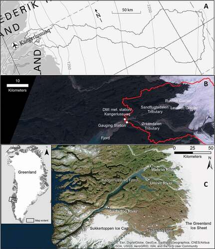
The Watson River catchment consists of two parts: an ice-sheet sector, stretching westward from the main GrIS topographic divide to the margin located approximately 30 km east of Kangerlussuaq Airport, and a proglacial area from the ice-sheet margin to the Kangerlussuaq river-gaging station (Figure 1). The catchment area is approximately 12,600 km² (of which 95 percent are glacierized) compared to the 9,743 km² used in the calculations of specific transport by Hasholt et al. (2013) and Yde et al. (2014). The 29 percent increase in estimated catchment area is the result of new information about the bedrock topography beneath the GrIS (Lindbäck et al. 2015). The proglacial area remains identical to the previous reported value (590 km²). The gaging station is located 300 m upstream of the Watson River outlet, where the river enters the delta area and the fjord Kangerlussuaq. Three kilometers upstream of the station, two river branches merge from Sandflugtsdalen and Ørkendalen. The rivers from these valleys originate at the ice-sheet margin 30–40 km upstream from the gaging station. The proglacial area represents a typical Greenlandic landscape (Anderson et al. 2002, 2017) with outwash plains, low vegetation, and permafrost and a coastal area connected to a delta and a fjord or ocean. The Sandflugtsdalen branch has at least three riegels across the river with braided reaches in between, whereas the Ørkendalen branch is braided along its entire reach.

Figure 1. (A) GrIS catchment after Lindbäck et al. (2015); (B) proglacial area; and (C) Watson River and the fjord Kangerlussuaq

The riegels and the rocks in the proglacial catchment consist mainly of gneiss of Nagsugtoqidian orogeny (Henriksen 2005). The main minerals comprise quartz, plagioclase, K-feldspar, amphibole, pyroxene, and pyrite with minor amounts of biotite, muscovite, garnet, magnetite, epidote, and chlorite (Hindshaw et al. 2014; Yde et al. 2010). Calcite does not occur as a primary mineral, but disseminated calcite has been recorded in very low trace amounts as a product of plagioclase weathering (Hindshaw et al. 2014). Evaporites have not been reported from this part of Greenland. The landscape consists of gently rolling bedrock hills with altitudes up to 600 m above sea level (a.s.l.), often covered by a thin layer of glacial deposits. Lakes and river valleys are incised between the hills. The river valleys are filled with braided river deposits (Carrivick et al. 2013) and in the western part are bordered by old marine terraces (Ten Brink 1974). The soils are classified as Haplic Cambisols (Jones et al. 2010). The vegetation consists mainly of grass and low scrub.

The climate of the GrIS in the region is monitored by automatic weather stations (AWS) located at a transect perpendicular to the ice-sheet margin (van As et al. 2017; van den Broeke et al. 2008). The glacial mean equilibrium line altitude (ELA) was reported to be approximately 1,550 m a.s.l. for 1991–2011 (van de Wal et al. 2012), but since 2010 has increased to altitudes between 1,500 and 1,850 m a.s.l. (Smeets et al. 2018; van As et al. 2017). Melting occurred as high as the main divide in 2012 (e.g., Hanna et al. 2014). The climate of the proglacial area is observed at Kangerlussuaq airport. Here, the mean annual air temperature, relative humidity, and wind speed were −3.3°C, 67 percent, and 3.7 m s⁻¹, respectively, for the period 1961–1990 (Cappelen 2016). The mean annual precipitation is 256 ± 60 mm w.e. for 1991 − 2012 after undercatch correction (Mernild et al. 2015). The climate is defined as low Arctic, according to Born and Böcher (2001). The presence of saline lakes as described by Anderson et al. (2002) indicates that the ice-free area is dry, and that runoff and sediment transport from the area outside the large valleys are negligible compared to the contributions from the GrIS. The winter precipitation accumulates as snow from October to May. The snow melts first at the lower altitudes in the proglacial area, causing a minor discharge peak in May–June. Because of the arid conditions, there is practically no runoff or sediment transport from the proglacial area the rest of the year. The main runoff season is from June to August following the melt, with secondary peaks caused by periods with intense melting, rainfall events, and/or sudden release of meltwater storage (glacial outbursts; Bartholomew et al. 2011; Russell et al. 2011; van As et al. 2017, 2018).

Methods

Discharge

Continuous recording of the river stage is carried out using DIVER pressure transducers that are corrected for barometric pressure. Since 2006 pressure transducers have been installed on a rock promontory approximately 150 m upstream of the bridge segments over the Watson River. During the first year, the measuring range of the pressure transducer was insufficient at 5 m, causing a data gap during the peak of the melt season. All later installed pressure transducers have a range of 10 m, and they record every five or ten minutes (accuracy ± 1–2 cm).

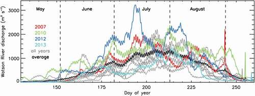
New discharge measurements are carried out using an ADCP and moving boat technique at a safe cross-section downstream of the riegel (Figure 2). The new discharge data have been used together with simultaneous stage records to establish a stage-discharge relation that was used to convert the continuous stage record into a continuous discharge record, accurate within 15 percent (60% for 2006; van As et al. 2017). Previously, the stage-discharge relation was based on less precise discharge measurements carried out using the float method (Hasholt et al. 2013). The recalculated annual discharge is roughly double the previous reported values. The large seasonal variations of the discharge within the different years appear in Figure 3 (van As et al. 2018).

Figure 2. Gaging station at bridge crossing during low runoff (April 19, 2016) and high runoff (July 25, 2016)

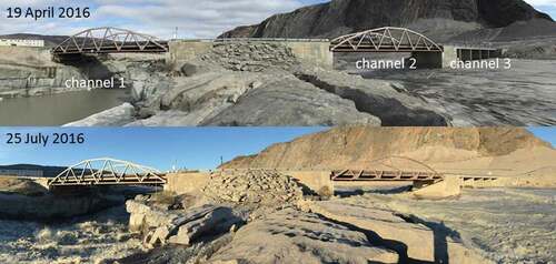
Figure 3. Seasonal variations of discharge. Years 2007, 2010, 2012, and 2013 are shown specifically. Peaks in August–September are jökulhlaup events (e.g., 2007)

Sediment flux

Water samples were collected using hand sampling with a bottle sampler (300–1,000 ml sample sizes). An ISCO 6700 peristaltic pump sampler (300 ml) was installed periodically. In all, since 2006 503 daily samples were collected at the Watson River bridge (Figure 2). Because of the extremely turbulent flow conditions on the riegel underneath the bridges (Froude numbers greater than 1, velocities 2–10 m s⁻¹), sediment with grain sizes up to at least 2 mm are homogeneously mixed with water throughout the cross-sections (Hasholt et al. 2013). During the major part of the runoff season, when the water velocity is well above 2 m s⁻¹, coarse sand (≥0.6 mm) is observed in the water samples. This implies that a simple bottle sampler can be used to obtain water samples representing the total sediment load, and that there is no need to use depth-integrated sampling of the suspended load and separate measurements of bed load. Analyses of the water samples for the determination of sediment concentration, loss on ignition, and grain size are described in detail by Hasholt et al. (2013). The accuracy of the determination of concentration is ±1 mg l⁻¹, which is negligible compared to observed short time variations of the concentrations of ±10 percent of mean.

A continuous record of sediment flux can then be derived by multiplying sediment concentration by the water flux. A continuous record of sediment concentration can be obtained through interpolation (Method 1) in Table 1, if sampling intervals are short enough for this method. We calculate annual total values for years with at least twenty-five samples taken throughout the entire melt season to interpolate between years (2008 to 2013).

Table 1. Modeled transport characteristics of sediment and solutes in Watson River

	2006	2007	2008	2009	2010	2011	2012	2013	2014	2015	2016	Average	SD
Discharge (km^3 a^−1)	5.4	7.5	5.5	4.9	11.2	7.8	10.7	4.3	6.8	3.8	8.1	6.9	2.5
Sediment
Number of samples	7	24	50	67	184	48	77	29		1	16
Mean concentration (mg l^−1)	1930	3011	1917	2400	2358	2350	2638	1369		1568	1369	2089	552
Maximum concentration (mg l^−1)	8255	5427	6257	5943	5117	4095	5113	4264		1568	3163	4920	1817
Method 1 (× 10^6 t a^−1)			9.3	10.6	26.4	21.0	28.4	10.2				17.6	8.7
Method 2 (× 10^6 t a^−1)	13.1	19.1	13.1	12.7	24.6	20.5	30.5	7.9	13.9	7.8	18.6	16.5	6.9
Method 3 (× 10^6 t a^−1)	13.1	19.4	13.2	11.4	29.6	20.2	29.3	10.2	16.9	8.7	20.9	17.5	7.2
Method deviation (%)	0	2	22	10	10	1	4	16	10	6	6	4
Specific transport (t km^−2 a^−1)	1040	1537	1038	909	2353	1606	2325	810	1345	693	1658	1392	573
Solutes
Total solute export(× 10^3 t a^−1)	66.5	84.7	70.7	60.8	138.2	95.6	132.0	53.9	83.1	46.6	99.8	84.7	29.9
Specific transport(t km^−2 a^−1)	5.3	6.7	5.6	4.8	11.0	7.6	10.5	4.3	6.6	3.7	7.9	6.7	2.4

To account for temporal variations of sediment concentration between sampling times, from 2007 to 2016 a Solitech transmissometer sensor and an OBS3+ optical backscatter sensor were installed periodically (and damaged or destroyed several times) under the northern bridge segment, measuring every five or ten minutes (channel 1 in Figure 2). The sensor signals provide proxies of sediment concentration (Method 2), but the signals must be calibrated against the concentrations from manual or ISCO water samples. The calibration curves following Hasholt et al. (2013) are shown in Figures 4B and 4C. Gaps in the record are filled using either Method 1 or Method 3 below. Method 2 provides us with ten years of sediment transport estimates (2007–2016).

Figure 4. (A) Sampled sediment concentration plotted against river discharge. The red line represents the best exponential fit; dashed lines give the root mean square difference. (B) Sediment concentration versus OBS sensor readings. The red line is the fit following Hasholt et al. (2013). (C) Sediment concentration versus Solitech sensor readings. The red line is the fit following Hasholt et al. (2013)

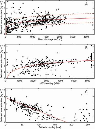
A third method (Method 3) of calculating sediment transport works for the entire 2006–2016 observational period and uses a newly derived empirical relation of sampled sediment concentration C(kg m⁻³) as a function of discharge Q (in m³ s⁻¹), C = 0.76 × Q^0.167 (Figure 4A), allowing sediment transport to be calculated using the continuous discharge record alone.

The accuracy of Methods 2 and 3 is ±25 percent. All sediment-transport calculations are described in more detail by Hasholt et al. (2013). For years with overlapping time series, the three methods give similar results and the differences are smaller than the uncertainty of the measurements (Table 1).

Solute flux

Bulk water samples were collected at the bank of the Watson River within a few hundred meters upstream from the gaging station. Here, we use a compiled set of solute data, consisting of sixty-four previously published analyses from 2007 to 2009 (described in detail by Yde et al. 2014), together with thirteen analyses from samples from 2013. We only include samples collected during the peak flow period in July and August because inclusion of samples collected during the early and late melt season may cause an overestimation of annual transports (Krawczyk, Lefauconnier, and Pettersson 2003; Stachnik et al. 2016; Yde et al. 2008). We present concentrations and transport of major ions (Na⁺, K⁺, Ca²⁺, Mg²⁺, Cl⁻, SO₄^2-, NO₃⁻, HCO₃⁻) and Si and Fe (see Yde et al. [2014] for details about the methods of ion analyses). The analytical uncertainties are as much as ±10 percent for some ions (K⁺, Ca²⁺, and Si), but generally less than ±5 percent (Yde et al. 2014). Some ion concentrations were not analyzed in 2008 (Fe), 2009 (Cl⁻, NO₃⁻, HCO₃⁻), and 2013 (Si, NO₃⁻, SO₄^2-, HCO₃⁻).

We use the discharge-weighted method, where measured ion concentrations are multiplied by the discharge at the time of sampling. The resulting instantaneous ion fluxes are then averaged and divided by the mean annual discharge average to derive annual mean ion concentrations. Annual ion exports are subsequently estimated by multiplying the annual mean ion concentrations with annual total discharge. These are used to calculate annual solute fluxes for years with measured ion concentrations. The mean ion concentrations of the measured years are used for the calculation of annual solute fluxes for years without measured ion concentrations. Differences are only as much as 2.4 percent between the new estimates of annual mean ion concentrations and the values used by Yde et al. (2014) for 2007, where ion concentrations were measured.

Results

The average annual sediment transport through the Watson River for 2006–2016 was 17.5 × 10⁶ t a⁻¹, with a maximum of 29.6 × 10⁶ t a⁻¹ in 2010 and a minimum of 8.7 × 10⁶ t a⁻¹ in 2015 (Table 1, Method 3). The standard deviation of the mean was 7.2 × 10⁶ t a⁻¹, indicative of a large interannual variability (Figure 5). No significant trend could be detected from the eleven-year observation period. The average specific sediment load was 1.39 × 10³ ± 0.2–0.3 × 10³ t km⁻² a⁻¹, with a maximum of 2.33 × 10³ t km⁻² a⁻¹, a minimum of 0.69 × 10³ t km⁻² a⁻¹, and a standard deviation of 0.57 × 10³ t km⁻² a⁻¹.

Figure 5. Annual totals and uncertainty of sediment transport through the Watson River

Characteristics of the transported sediment are shown in Table 2. The average loss on ignition was 1.3 percent of the sediment transport, with a maximum of 2.7 percent and a minimum of 0.2 percent during the eleven-year period. The lowest percentage was found when the transport was high. The concentration of sediment that passed the 0.7 µm glass fiber filters and was captured on the 0.45 µm membrane filters was in average 15 mg l⁻¹, or less than 1 percent of the average sediment concentration (Table 2). It is not possible to give a thorough description of the seasonal variations, because these measurements only covered five years and did not include all water samples. However, the highest concentrations of very fine sediment mainly occurred in samples collected early in the peak flow season and during the autumn recession. Very low concentrations occurred in samples from the mid-peak flow season, indicating a supply limit of very fine material. Grain-size distributions from 2009 (low discharge) showed that 71 percent of the sediment was finer than medium silt (20 µm) while only 7.5 percent was finer in 2010 (high discharge; Table 2). Coarser particles (pebble size) were not observed in the water samples, but a transport of pebble-size material at the gaging station was observed as pebbles either wedged into the sensor fittings or imbedded in drifting ice floes. The grain-size distributions clearly demonstrate not only that the transport consisted of a large proportion of very fine material but also that years with high flood discharges carried coarser sediment, 21 percent was coarse sand or coarser in 2010 while it was 0 percent in 2009.

Table 2. Characteristics of sediments and solutes in Watson River, 2006–2016. Solute concentrations are shown as annual-mean ion concentrations based on the discharge-weighted method

	2006	2007	2008	2009	2010	2011	2012	2013	2014	2015	2016	Average	Stdev
Average loss on ignition (%)	1.9	1.5	1.2	1.2	1.2	0.4	0.2	2.7		1.0	1.4	1.27	0.71
Maximum (%)	3.2	1.9	4.7	6.0	3.5	2.2	0.69	6.9			3.0	3.57	1.99
Minimum (%)	1.1	1.2	0.4	0.4	0.4	0.02	0.1	0.7			0.4	0.52	0.41
Average 0.7–0.45 μm fraction (mg l^−1)	7.7	13.9	9.5	0	44.3							15.1	15.3
Maximum (mg l^−1)	11.7	15.5	44.8	0	68.9							28.2	25.1
Minimum (mg l^−1)	1.8	12.4	0	0	21.2							7.1	8.4
Average grain size (µm)				8.9	154.8
Max. (μm)				13.9	227.9
Min. (μm)				5.4	118.3
<20 μm fraction (%)				71	7.5
Na^+ mg l^−1		0.75	0.84	0.81				0.76				0.79	0.002
K^+ mg l^−1		0.79	0.92	0.89				1.05				0.91	0.006
Ca^2+ mg l^−1		1.32	1.68	1.79				2.14				1.73	0.19
Mg^2+ mg l^−1		0.20	0.20	0.25				0.33				0.25	0.003
Cl^− mg l^−1		1.07	1.02					0.44				0.84	0.15
NO3^− mg l^−1		0.15	0.16									0.15	0.0002
SO4^2- mg l^−1		1.54	1.77	1.55								1.62	0.006
HCO3^− mg l^−1		4.32	5.65									4.98	0.29
Si mg l^−1		1.07	0.65	1.17								0.96	0.12
Fe mg l^−1		0.08		0.03				0.05				0.05	0.01

The average annual solute transport was 85 × 10³ t a⁻¹ (with standard deviation of 30 × 10³ t a⁻¹); that is, 200 times smaller than the sediment transport (Table 1). We find a maximum annual solute transport of 138 × 10³ t a⁻¹ in 2010, and a minimum of 47 × 10³ t a⁻¹ in 2015. The corresponding average specific solute yield was 6.7 t km⁻² a⁻¹ with a standard deviation of 2.4 t km⁻² a⁻¹. The major ions constituted approximate 92 percent of the total annual solute transport. The dominating anion and cation were HCO₃⁻ and Ca²⁺, respectively (Table 2). For most ions, the average ion concentration shows little variation in years with measurements.

Discussion and conclusions

Given our discharge-independent methodology for sediment concentration determination (Methods 1 and 2), the sediment flux is directly proportional to the discharge. The new annual mean (17.5 × 10⁶ t a⁻¹) is 10.2 × 10⁶ t a⁻¹ larger than the previously published 7.3 × 10⁶ t a⁻¹ in Hasholt et al. (2013). This is partly because of the extension of the monitoring period, but mostly because of the new stage discharge relationship by van As et al. (2017), roughly doubling the discharge. The updated mean specific yield (1.39 × 10³ t km⁻² a⁻¹) is larger than the previously published value of 0.744 × 10³ t km⁻² a⁻¹, despite using a 29 percent larger catchment area in our calculations.

Previous investigations of the sediment and solute flux in the Watson River catchment were carried out at the Leverett Glacier, draining a 600 km² subcatchment of the Kangerlussuaq area. Cowton et al. (2012) describe flux and specific yield from the years 2009 and 2010. Their results are included in the extended time series covering the years 2011 and 2012 by Hawkings et al. (2015). They state that the fluxes of sediment do not scale with discharge because the subglacial drainage network does not always give access to the eroded sediment that can be transported. They also find specific total sediment yields of as much as 15,000 t km⁻² a⁻¹, larger than all other specific yields measured in Greenland (Hasholt 2016). Presumably intense subglacial erosion takes place near the margin of the ice sheet where ample meltwater flushes the eroded material, in contrast to more interior locations where meltwater is not (abundantly) present. The methodology by Cowton et al. (2012) and Hawkings et al. (2015) differs from ours by only measuring suspended load and not covering the complete month of September.

The Kangerlussuaq Fjord receives sediment originating from both the GrIS and the proglacial area. The contribution from most of the approximately 590 km² proglacial area, consisting of vegetation-covered soil and some bare rock, is negligible. Yet the approximately 50 km² outwash plains in the proglacial valleys likely function as considerable sources and sinks. We estimate the mass balance of these outwash plains by subtracting the measured sediment output to the sea by the input from the GrIS that we can base on previous findings following Cowton et al. (2012) and using their reported contribution from the Leverett Glacier subcatchment and uncertainties. We upscale to encompass the entire Kangerlussuaq catchment by assuming the same annual specific yield throughout the ice-sheet ablation area as from the Leverett Glacier catchment (600 km²). The Russell Glacier part of the Sandflugtsdalen catchment contributes with 58 km², partly based on Lindbäck et al. (2015). The contribution from the Ørkendalen GrIS tributary is found using the 1,800 km² ablation area from Lindbäck et al. (2015). We use the 600 km² Leverett Glacier catchment area reported by Cowton et al. (2012) instead of the 900 km² found by Lindbäck et al. (2015). The calculated annual mass balance for the four years (2009–2012) with overlapping measurements is shown in Table 3. The results suggest that the proglacial outwash plains act as net sinks in years with low melt runoff and as net sources during years with high meltwater runoff from the GrIS. Glacial erosion causes accumulation of eroded material at the bottom of the GrIS. The uptake of eroded sediments depends on the development level of the subglacial drainage network. If the meltwater transport capacity exceeds the amount of available sediment, the flux will decrease with increasing discharge. On the outwash plains, the rivers are alluvial (Engelund and Hansen 1972). Because river velocity and bed-shear stress increase with increasing discharge and sediment is abundant on the alluvial plains, the sediment flux here will increase too. The resultant net depositions from the four-year mass balance indicate that an average of 6 cm is deposited upon the approximately 50 km² outwash plains (Table 3). The increased contribution from the outwash plains at high discharge is indicated by the larger amount of coarse sediment in 2010 compared to 2009 (Table 2). This is also supported by the increase in delta areas at Kangerlussuaq and around Greenland. Bendixen et al. (2017) relate the increasing delta areas, contrasting the observed coastal erosion in other Arctic areas to the recent increases in meltwater runoff from Greenland. Watson River discharge estimates for 1949–2016 confirm that meltwater production has been relatively low and rather stable until 2000, followed by a substantial increase (van As et al. 2018).

Table 3. Sediment annual mass balance estimates for the Watson River catchment, 2009–2012

		Leverett Glacier		Russell Glacier	Ørkendalen Tributary	Total GrIS Input	Watson River Export			Proglacial Deposition
Year	Specific Sediment Transport	Sediment Transport^a	Uncertainty^a	Sediment Transport	Sediment Transport	Sediment Transport	Sediment Transport	Uncertainty	Specific Sediment Transport	Sediment Loss
	(t km^−2 a^−a)	(x 10^6 t a^−a)		(x 10^6 t a^−a)	(x 10^6 t a^−a)	(x 10^6 t a^−a)	(x 10^6 t a^−a)		(t km^−2 a^−a)	(× 10^6 t a^−a)
2009	15,000	9	±39%	0.53	27	36.5	11.4	±25%	910	25.1
2010	10,100	6	±39%	0.35	18.2	24.6	29.6	±25%	2,350	−5.0
2011	11,700	7	±39%	0.41	21	28.4	20.2	±25%	1,610	8.2
2012	8,500	5	±39%	0.30	15.3	20.7	29.3	±25%	2,330	−8.6
Average	11,300	6.8				27.6	22.6		1,800	4.9
SD	2,800	1.7				6.7	8.7		690	15.3

^aFrom Cowton et al. (2012) and Hawkings et al. (2015)

An estimate of the total contribution of sediment to the Kangerlussuaq fjord was presented by Mikkelsen and Hasholt (2013). It was found that the specific load from the Sarfartoq catchment (Figure 1C) was only a third of the specific load from the Kangerlussuaq (Watson River) and Umivit catchments, because a share of the sediment from the GrIS part of the Sarfartoq catchment is collected in a large proglacial lake. The new stage-discharge relation and the changed catchment area for Watson River only increase this difference, revealing the importance of proglacial sediment sinks.

Previously published total solute transport and major ion values (2007–2010) were 44 and 40 × 10³ t a⁻¹, respectively (Yde et al. 2014), compared to 89 and 81 × 10³ t a⁻¹ for the same period using the new discharge dataset. Although there are only a few years of overlap between our values and those reported by Hawkings et al. (2015), they correlate well (r² = 0.88) and both scale to discharge. The findings support that increasing discharge leads to increased export of solutes and related nutrients from the Watson River catchment.

We find an average specific solute transport of 6.7 t km² a⁻¹. This specific transport is lower than any other previous estimations of the specific total solute flux from glacierized catchments (Tranter and Wadham 2014). This may partly be because of limited influence from subglacial water beneath the accumulation area and partly because of chemical depletion of subglacial sediment (Graly, Humphrey, and Harper 2016).

In recent years, there has been an increasing effort to quantify the magnitudes of chemical transport from the GrIS to adjacent seas, with special emphasis on nutrient export (e.g., Hawkings et al. 2014, 2015, 2016, 2017; Wadham et al. 2016). These estimates are almost all based on an upscaling from the Watson River catchment, or the subcatchment Leverett Glacier, to the entire GrIS. Because of the relatively low chemical reactivity of the local gneissic lithology and the low input of marine-derived salts, the estimated ion exports from the GrIS should be regarded as conservative estimates. In Table 4, we present past, present, and future estimates of ion export from the GrIS, based on GrIS runoff modeling estimates derived by Lenaerts et al. (2015). The GrIS runoff was calculated from the estimated total freshwater runoff subtracted by solid-ice calving (520 Gt yr⁻¹) and seasonal snowmelt from the tundra (50 Gt yr⁻¹), assuming that the contributions from both solid-ice calving and seasonal snowmelt from the tundra remain constant through time (Lenaerts et al. 2015). Between the periods 1960–1989 and 2006–2016, the runoff from the GrIS has increased by 65 percent. Assuming that runoff is the dominant control on solute export (Tranter and Wadham 2014), this increase in runoff is equivalent to a 65 percent increase in solute export. For estimations of future solute exports, the climate-change scenario Representative Concentration Pathways 2.6 (RCP2.6) is applied to present an increasing atmospheric temperature (c. 2 K) over Greenland until the year 2100, followed by a slow decrease (Lenaerts et al. 2015). In contrast, the climate-change scenario RCP8.5/4xCO₂ represents a situation with increasing atmospheric CO₂ concentration to four times the preindustrial level in 2120 (c. 5 K in 2100), followed by a stable atmospheric CO₂ concentration (Lenaerts et al. 2015).

Table 4. Past, present, and future estimates of ion fluxes (× 10³ t yr⁻¹) from the GrIS based on upscaling from the Watson River catchment. The mean GrIS runoff fluxes are derived from Lenaerts et al. (2015). Two climate scenarios are used for estimating future ion fluxes. The RCP2.6 scenario has a modest increase in atmospheric temperature over Greenland until 2100 (c. 2 K), followed by a slow decrease. The RCP8.5/4xCO₂ scenario has a strong increase in atmospheric temperature over Greenland (c. 5 K in 2100)

	Runoff	Na^+	K^+	Ca^2+	Mg^2+	Cl^−	NO3^−	SO4^2-	HCO3^−	Si	Fe
	(km^3 yr^−1)	(× 10^3 t yr^.1)
1960–1989	394	311	358	677	96	337	60	640	1,959	380	20
2006–2016	652	515	592	1,120	159	557	98	1,059	3,241	629	33
2090–2099 (RCP2.6)	800	631	727	1,374	195	684	121	1,299	3,975	772	41
2090–2099 (RCP8.5/4xCO2)	1,581	1,247	1,435	2,715	384	1,350	239	2,565	7,853	1,525	81

The low-emission RCP2.6 scenario indicates a 23 percent increase in solute export in the years 2090–2099 from the contemporary level during 2006–2016, whereas the high-emission RCP8.5/4xCO₂ scenario shows a 142 percent increase in solute export. A change in GrIS solute export to this level is likely to have a huge impact on the marine primary productivity in the North Atlantic Ocean (e.g., Hawkings et al. 2015), especially considering that a simultaneous increase in suspended sediment export will lead to an even higher availability of labile nutrients to the surrounding seas (Gíslason, Oelkers, and Snorrason 2006; Hawkings et al. 2015; Hodson, Mumford, and Lister 2004). Changes in nutrient export from the GrIS will affect global biogeochemical cycles and related climatic feedback mechanisms. For instance, Meire et al. (2016) found that a high export of dissolved Si from the GrIS is likely to stimulate diatom growth, and thus primary production, in near-coastal ecosystems. Our Si estimate of 629 × 10³ t a⁻¹ supports the magnitude of their estimate of 618 × 10³ t a⁻¹. In combination with contributions from amorphous Si (Hawkings et al. 2017, 2015) and aeolian dust (Tréguer and De La Rocha 2013), a future increase in Si export will likely result in enhanced atmospheric carbon fixation by diatoms in the North Atlantic Ocean. The GrIS has also been identified as an important source for other macronutrients, such as phosphorus (Hawkings et al. 2016), nitrogen (Telling et al. 2012; Wadham et al. 2016), and iron (Bhatia et al. 2013; Hawkings et al. 2014; Statham, Skidmore, and Tranter 2008; Yde and Knudsen 2004; Yde et al. 2014), which potentially will stimulate increased marine primary production. Our Fe estimate of 33 × 10³ t a⁻¹ from the GrIS is similar in magnitude to previous estimates of 10 × 10³ t a⁻¹ (Bhatia et al. 2013), 16.5 × 10³ t a⁻¹ (Hawkings et al. 2014), and 15–52 × 10³ t a⁻¹ (Yde et al. 2014), but significantly higher than 1 × 10³ t a⁻¹ (Statham, Skidmore, and Tranter 2008). In order to present more accurate estimates, more hydrochemical data and discharge measurements are needed from chemically reactive basaltic catchments in west and east Greenland and sedimentary catchments in north and northeast Greenland.

Our results support that the GrIS is a major provider of sediments and solutes to both proglacial areas and to the sea. The average specific sediment yield (1,390 t km⁻² a⁻¹) from the 12,600 km² catchment is as high as for local glaciers in Greenland and elsewhere. Considering that the large upper part of the catchment where the ice sheet is frozen to the bed is not contributing at the moment, the specific sediment yield near the margin of the GrIS must be larger than for relatively small and thin local glaciers, supporting the findings of Cowton et al. (2012) and Hawkings et al. (2015). Our data span a longer time period and constrain the averages of fluxes and specific yields better than previous estimates. We therefore recommend that our estimates are taken into account when upscaling sediment production to the entire GrIS. Hasholt et al. (2006) already stated that Greenland was the major contributor of sediments and solutes to the surrounding seas. However, they argued that the estimate of the sediment contribution was not well constrained because of the poor measurement coverage, in addition to the unknown contribution of calving ice at marine-terminating glaciers. In recent years more information about sediment transport in Greenland has become available (e.g., Hasholt 2016; Ladegaard-Pedersen et al. 2017; Hawkings et al. 2017; Overeem et al. 2017). However, large areas in Greenland are still not monitored, and the calving contribution is still not well constrained. Our new estimate of solute transport is probably too low, because observations from more chemically reactive basaltic and sedimentary areas are missing. Our results show that estimates based on single years or short periods may cause considerable over- or underestimation, stressing the need for longer time series. If climate warming will yield increased amounts of meltwater, the contribution of sediment and solutes will increase proportionally. However, the amount of sediment that actually reaches the sea strongly depends on the sediment pathways through sink and source areas within the catchment.

Acknowledgments

We thank K. Lindbäck for the Kangerlussuaq catchment delineation, J. Lenaerts for providing the GrIS runoff estimates, and B. Fog and K. Pørksen for producing Figure 1. Thanks to K. Thorsøe, J. Abermann, and S. Wacker for retrieving CT and CTD loggers. Reviewers and associate editor, J. Telling, are thanked for critical comments improving the manuscript.

Additional information

Funding

Over the years, the Watson River discharge monitoring has been financed through various funding sources: the Commission for Scientific Research in Greenland grants 07-015998, 09-064628 and 2138-08-0003, the Danish Natural Science Research Council grant 272-07-0645, the Center for Permafrost (CENPERM), the Department of Geosciences and Natural Resource Management (IGN), the Greenland Analogue Project (GAP), and the Danish Energy Agency (ENS) through the WASEIS and PROMICE projects. We acknowledge local support by the Centre for Ice and Climate (CIC/NBI), CH2M HILL Polar Services (CPSpolar), Kangerlussuaq International Science Support (KISS), and the Greenland Survey (Asiaq).

References

- Anderson, N. J., J. E. Saros, J. E. Bullard, S. M. P. Cahoon, S. McGowan, E. A. Bagshaw, C. D. Barry, R. Bindler, B. T. Burpee, J. L. Carrivick, et al. 2017. The Arctic in the 21st century: Changing biogeochemical linkages across a paraglacial landscape of Greenland. BioScience 67:1–13.
- Anderson, N. J., S. Fritz, C. Gibson, B. Hasholt, and M. Leng. 2002. Lake-catchment interactions with climate in the low Arctic of southern West Greenland. Geological Survey of Greenland Bulletin 191:144–49.
- Bartholomew, I., P. Nienow, A. Sole, D. Mair, T. Cowton, S. Palmer, and J. Wadham. 2011. Supraglacial forcing of subglacial drainage in the ablation zone of the Greenland ice sheet. Geophysical Research Letters 38:L08502. doi:https://doi.org/10.1029/2011GL047063.
- Bendixen, M., L. L. Iversen, A. A. Bjørk, B. Elberling, A. Westergaard-Nielsen, I. Overeem, K. Barnhart, S. A. Khan, J. E. Box, J. Abermann, et al. 2017. Delta progradation in Greenland driven by increasing glacial mass loss. Nature 550:101–4. doi:https://doi.org/10.1038/Nature23873.
- Bhatia, M. P., E. B. Kujawinski, S. B. Das, C. F. Breier, P. B. Henderson, and M. A. Charette. 2013. Greenland meltwater as a significant and potentially bioavailable source of iron to the ocean. Nature Geoscience 6:274–78.
- Born, E., and J. Böcher. 2001. The ecology of Greenland. Nuuk: Ministry of Environment and Natural Resources.
- Cappelen, J. 2016. Weather observations in Greenland 1958–2015. Copenhagen: Danish Meteorological Institute Report 16-08, 31.
- Carrivick, J. L., A. G. D. Turner, A. J. Russell, T. Ingeman-Nielsen, and J. C. Yde. 2013. Outburst flood evolution at Russell Glacier, western Greenland: Effects of a bedrock cascade with intermediary lakes. Quaternary Science Reviews 67:39–58.
- Cowton, T., P. Nienow, I. Bartholemew, A. Sole, and D. Mair. 2012. Rapid erosion beneath the Greenland Ice Sheet. Geology 40:343–46.
- Engelund, F., and E. Hansen. 1972. A monograph on sediment transport in alluvial streams. Teknisk Forlag, Copenhagen, Denmark. 62 pp.
- Gíslason, S. R., E. H. Oelkers, and Á. Snorrason. 2006. Role of river-suspended material in the global carbon cycle. Geology 34:49–52.
- Graly, J. A., N. F. Humphrey, and J. T. Harper. 2016. Chemical depletion of sediment under the Greenland Ice Sheet. Earth Surface Processes and Landforms 41:1922–36.
- Hallet, B., L. Hunter, and J. Bogen. 1996. Rates of erosion and sediment evacuation by glaciers: A review of field data and their implications. Global and Planetary Change 12:213–35.
- Hanna, E., X. Fettweis, S. H. Mernild, J. Cappelen, M. Ribergaard, C. Shuman, K. Steffen, L. Wood, and T. Mote. 2014. Atmospheric and oceanic climate forcing of the exceptional Greenland Ice Sheet surface melt in summer 2012. International Journal of Climatology 34:1022–37.
- Hasholt, B. 2016. Sediment and solute transport from Greenland. In Source-to-sink fluxes in undisturbed cold environments, ed. A. Beylich, J. C. Dixon, and Z. Zwolinski, 96–115. Cambridge: Cambridge University Press.
- Hasholt, B., N. Bobrovitskaya, J. Bogen, J. McNamara, S. H. Mernild, D. Milburn, and D. E. Walling. 2006. Sediment transport to the Arctic Ocean and adjoining cold oceans. Nordic Hydrology 37:413–32.
- Hasholt, B., A. B. Mikkelsen, M. H. Nielsen, and M. A. D. Larsen. 2013. Observations of runoff and sediment and dissolved loads from the Greenland Ice Sheet at Kangerlussuaq, West Greenland, 2007 to 2010. Zeitschrift Für Geomorphologie 57 (Suppl. 2):3–27.
- Hawkings, J., J. Wadham, M. Tranter, J. Telling, E. Bagshaw, A. Beaton, S.-L. Simmons, D. Chandler, A. Tedstone, and P. Nienow. 2016. The Greenland Ice Sheet as a hot spot of phosphorus weathering and export in the Arctic. Global Biogeochemical Cycles 30:191–210. doi:https://doi.org/10.1002/2015GB005237.
- Hawkings, J. R., J. L. Wadham, L. G. Benning, K. R. Hendry, M. Tranter, A. Tedstone, P. Nienow, and R. Raiswell. 2017. Ice sheets as a missing source of silica to the polar oceans. Nature Communications 8:14198. doi:https://doi.org/10.1038/ncomms14198.
- Hawkings, J. R., J. L. Wadham, M. Tranter, E. Lawson, A. Sole, T. Cowton, A. J. Tedstone, I. Bartholomew, P. Nienow, D. Chandler, et al. 2015. The effect of warming climate on nutrient and solute export from the Greenland Ice Sheet. Geochemical Perspectives Letters 1:94–104.
- Hawkings, J. R., J. L. Wadham, M. Tranter, R. Raiswell, L. G. Benning, P. J. Statham, A. Tedstone, P. Nienow, K. Lee, and J. Telling. 2014. Ice sheets as a significant source of highly reactive nanoparticulate iron to the oceans. Nature Communications 5:3929. doi:https://doi.org/10.1038/ncomms4929.
- Henriksen, N. 2005. Grønlands geologiske udvikling. Copenhagen: Geological Survey of Denmark and Greenland (GEUS), 270.
- Hindshaw, R. S., J. Rickli, J. Leuthold, J. Wadham, and B. Bourdon. 2014. Identifying weathering sources and processes in an outlet glacier of the Greenland Ice Sheet using Ca and Sr isotope ratios. Geochimica Et Cosmochimica Acta 145:50–71.
- Hodson, A. J., P. Mumford, and D. Lister. 2004. Suspended sediment and phosphorus in proglacial rivers: Bioavailability and potential impacts upon the P status of ice-marginal receiving waters. Hydrological Processes 18:2409–22.
- Hudson, B., I. Overeem, D. McGrath, J. P. M. Syvitski, A. B. Mikkelsen, and B. Hasholt. 2013. MODIS observed increase in the duration and spatial extent of sediment plumes in Greenland fjords. The Cryosphere Discussions 7:6101–41.
- Jones, A., V. Stolbovoy, C. Tarnocai, G. Broll, O. Spaargaren, and L. Montanarella. 2010. Soil atlas of the northern circumpolar region. Luxembourg: European Commission, Publications Office of the European Union.
- Koppes, M. N., and D. R. Montgomery. 2009. The relative efficacy of fluvial and glacial erosion over modern orogenic timescales. Nature Geoscience 2:644–47.
- Krawczyk, W. E., B. Lefauconnier, and L.-E. Pettersson. 2003. Chemical denudation rates in the Bayelva catchment, Svalbard, in the fall of 2000. Physics and Chemistry of the Earth 28:1257–71.
- Ladegaard-Pedersen, P., C. Sigsgaard, A. Kroon, J. Aberman, K. Skov, and B. Elberling. 2017. Suspended sediment in a high-Arctic river: An appraisal of flux estimation methods. Science of the Total Environment 580:582–92. doi:https://doi.org/10.1016/j.scitotenv.2016.12.006.
- Lenaerts, J. T. M., D. Le Bars, L. van Kampenhout, M. Vizcaíno, E. M. Enderlin, and M. R. van den Broeke. 2015. Representing Greenland Ice Sheet freshwater fluxes in climate models. Geophysical Research Letters 42:6373–81.
- Lindbäck, K., R. Pettersson, A. L. Hubbard, S. H. Doyle, D. van As, A. B. Mikkelsen, and A. A. Fitzpatrick. 2015. Subglacial water drainage, storage, and piracy beneath the Greenland Ice Sheet. Geophysical Research Letters 42:7606–14.
- McGrath, D., K. Steffen, I. Overeem, S. H. Mernild, B. Hasholt, and M. van den Broeke. 2010. Sediment plumes as proxy for local ice-sheet runoff in Kangerlussuaq Fjord, West Greenland. Journal of Glaciology 56 (199):813–21.
- Meire, L., P. Meire, E. Struyf, D. W. Krawczyk, K. E. Arendt, J. C. Yde, T. J. Pedersen, M. J. Hopwood, S. Rysgaard, and F. J. R. Meysman. 2016. High export of dissolved silica from the Greenland Ice Sheet. Geophysical Research Letters 43:9173–82.
- Mernild, S. H., E. Hanna, J. R. McConnell, M. Sigl, A. P. Beckerman, J. C. Yde, J. Cappelen, and K. Steffen. 2015. Greenland precipitation trends in a long-term instrumental climate context (1890–2012): Evaluation of coastal and ice core records. International Journal of Climatology 35:303–20.
- Mikkelsen, A. B., and B. Hasholt. 2013. Sediment transport to the Kangerlussuaq fjord, west Greenland. In Proceedings 19th International Research Basins Symposium and Workshop, ed. S. L. Stuefer and W. R. Bolton, 157–66. University of Alaska Fairbanks, Fairbanks, USA.
- Overeem, I., B. D. Hudson, J. P. M. Syvitski, A. B. Mikkelsen, B. Hasholt, M. R. den Broeke, B. P. Y. Noël, and M. Morlighem. 2017. Substantial export of suspended sediment to the global oceans from glacial erosion in Greenland. Nature Geoscience 10:859–63.
- Russell, A. J., J. L. Carrivick, T. Ingeman-Nielsen, J. C. Yde, and M. Williams. 2011. A new cycle of jökulhlaups at Russell Glacier, Kangerlussuaq, West Greenland. Journal of Glaciology 57 (202):238–46.
- Smeets, C. J. P. P., P. Kuipers Munneke, D. van As, M. R. van den Broeke, W. Boot, J. Oerlemans, H. Snellen, C. H. Reijmer, and R. S. W. van de Wal. 2018. The K-transect in west Greenland: Twenty-three years of weather station data. Arctic, Antarctic, and Alpine Research, in press.
- Stachnik, Ł., E. Majchrowska, J. C. Yde, A. P. Nawrot, K. Cichała-Kamrowska, D. Ignatiuk, and A. Piechota. 2016. Chemical denudation and the role of sulfide oxidation at Werenskioldbreen, Svalbard. Journal of Hydrology 538:177–93.
- Statham, P. J., M. Skidmore, and M. Tranter. 2008. Inputs of glacially derived dissolved and colloidal iron to the coastal ocean and implications for primary productivity. Global Biogeochemical Cycles 22:GB3013.
- Strahler, A. H., and A. N. Strahler. 1992. Modern physical geography. New York: John Wiley & Sons.
- Syvitski, J. P. M., J. T. Andrews, and J. A. Dowdeswell. 1996. Sediment deposition in an iceberg-dominated glacimarine environment, East Greenland: Bain fill implications. Global and Planetary Change 12:251–70.
- Telling, J., M. Stibal, A. M. Anesio, M. Tranter, I. Nias, J. Cook, C. Bellas, G. Lis, J. L. Wadham, A. Sole, et al. 2012. Microbial nitrogen cycling on the Greenland Ice Sheet. Biogeosciences 9:2431–42.
- Ten Brink, N. 1974. Glacio-isostasy: New data from West Greenland and geophysical implications. Geological Society of America Bulletin 85:219–28.
- Tranter, M., and J. L. Wadham. 2014. Geochemical weathering in glacial and proglacial environments. In Treatise on geochemistry, ed. H. D. Holland and K. K. Turekian, vol. 7, 2nd ed., 157–73. Oxford: Elsevier.
- Tréguer, P. J., and C. L. De La Rocha. 2013. The world ocean silica cycle. Annual Reviews of Marine Science 5:477–501.
- van As, D., A. Bech Mikkelsen, M. Holtegaard Nielsen, J. E. Box, L. Claesson Liljedahl, K. Lindbäck, L. Pitcher, and B. Hasholt. 2017. Hypsometric amplification and routing moderation of Greenland ice sheet meltwater release. The Cryosphere 11:1371–86. doi:https://doi.org/10.5194/tc-11-1371-2017.
- van As, D., B. Hasholt, A. P. Ahlstrøm, J. E. Box, J. Cappelen, W. Colgan, R. S. Fausto, S. H. Mernild, A. B. Mikkelsen, P. Y. N. Brice, et al. 2018. The longest observationally-constrained record of Greenland ice sheet meltwater discharge (1949–2016). Arctic, Antarctic, and Alpine Research (submitted), in press.
- van den Broeke, M., P. Smeets, J. Ettema, and P. K. Munneke. 2008. Surface radiation balancein the ablation zone of the west Greenland ice sheet. Journal of Geophysical Research 113:D13105.
- van de Wal, R. S. W., W. Boots, C. J. P. Smeets, H. Snellen, M. R. van den Broeke, and J. Oerlemans. 2012. Twenty-one years of mass balance observations along the K-transect, West Greenland. Earth System Science Data 4:31–35.
- Wadham, J. L., J. Hawkings, J. Telling, D. Chandler, J. Alcock, E. O’Donnell, P. Kaur, E. Bagshaw, M. Tranter, A. Tedstone, et al. 2016. Sources, cycling and export of nitrogen on the Greenland Ice Sheet. Biogeosciences 13:6339–52.
- Yde, J. C., K. W. Finster, R. Raiswell, J. P. Steffensen, J. Heinemeier, J. Olsen, H. P. Gunnlaugsson, and O. B. Nielsen. 2010. Basal ice microbiology at the margin of the Greenland ice sheet. Annals of Glaciology 51 (56):71–79.
- Yde, J. C., and N. T. Knudsen. 2004. The importance of oxygen isotope provenance in relation to solute content of bulk meltwaters at Imersuaq Glacier, West Greenland. Hydrological Processes 18:125–39.
- Yde, J. C., N. T. Knudsen, B. Hasholt, and A. B. Mikkelsen. 2014. Meltwater chemistry and solute export from a Greenland Ice Sheet catchment, Watson River, West Greenland. Journal of Hydrology 519:2165–79.
- Yde, J. C., M. Riger-Kusk, H. H. Christiansen, N. T. Knudsen, and O. Humlum. 2008. Hydrochemical characteristics of bulk meltwater from an entire ablation season, Longyearbreen, Svalbard. Journal of Glaciology 54 (185):259–72.