Reconstructing Greenland Ice Sheet meltwater discharge through the Watson River (1949–2017)

ABSTRACT

Ice-sheet melting is the primary water source for the proglacial Watson River in southern west Greenland. Discharge from the large, approximately 12,000 km² ice-sheet catchment draining through the Watson River has been monitored since 2006. While this record is of respectable length for a Greenland monitoring effort, it is too short to resolve climate signals. Therefore, we use observed Tasersiaq lake discharge and Kangerlussuaq air temperature to reconstruct annual Watson River discharge back to 1949. The resulting sixty-five-year record shows that average ice-sheet runoff since 2003 has roughly increased by 46 percent relative to the 1949–2002 period. The time series suggests that the five top-ranking discharge years occurred since 2003. The three top-ranking discharge years (2010, 2012, and 2016) are characterized by melt seasons that were both long and intense. Interannual variability more than doubled since 2003, which we speculate to be because of hypsometric runoff amplification enhanced by albedo decrease and decreased firn permeability. The reconstructed time series proves to be a valuable tool for long-term evaluation of Greenland Ice Sheet surface mass balance models. A comparison with freshwater fluxes calculated by a downscaled version of the regional climate model RACMO2 reveals high correlation (r = 0.89), and also shows that the model possibly underestimates runoff by up to 26 percent in above-average melt years.

KEYWORDS:

• Greenland Ice Sheet
• melt
• climate change
• measurements
• model validation
• Kangerlussuaq

Introduction

Discharge measurements of proglacial rivers in Greenland have provided valuable insights into ice-sheet surface mass balance (SMB), hydrology, and sediment release in recent years (e.g., Bendixen et al. 2017; Chandler et al. 2013; Doyle et al. 2015; Fitzpatrick et al. 2014; Langen et al. 2015; Lindbäck et al. 2015; Overeem et al. 2015; Rennermalm et al. 2013; Smith et al. 2015). Yet, despite a wide variety of applications, only a handful of Greenland proglacial river discharge monitoring sites exist. Difficulties in measuring discharge from the ice sheet include: (1) large seasonality in meltwater production (halting in winter), (2) extreme forces on submerged equipment during peak flow, (3) frost damage to submerged equipment outside the melt season, (4) a lack of stable bedrock for instrument mounting and deriving temporally stable stage-discharge relations, and (5) general inaccessibility of the Greenland proglacial area. Since 2006, a hydrometric station has operated in the settlement of Kangerlussuaq, located on the Watson River in southern west Greenland (Figure 1). The river drains a large, approximately 12,000 km² sector of the ice sheet (Lindbäck et al. 2015). Its discharge time series, and revisions thereof, have been presented by, for example, Hasholt et al. (2013) and Mikkelsen et al. (2016). This data record has been important for studies of, for example, ice-sheet surface melting, the glacial hydraulic system, and sediment production. However, the limited (currently twelve year) length of the data record hampers the interpretation of interannual discharge variability or peak discharge values in a multi-decadal, or truly climatic, context. The timing of the data record during a particularly warm period in Greenland history (Mernild et al. 2014; Cappelen 2017; van den Broeke et al. 2016; Figure 2) averages that ice-sheet meltwater discharge through the Watson River was likely considerably higher during the observational period than in preceding decades. This notion is anecdotally supported by the destruction of six-decade-old earthen bridge abutments during a July 2012 overbank flooding event in Kangerlussuaq. To date, only climate models are capable of estimating ice-sheet surface meltwater runoff during a time period of multiple decades, but the further back in time the simulations are pushed, the fewer atmospheric observations are available to both force and validate the models.

Figure 1. Map of the study area with ice-sheet catchments (Watson River catchment in red, Tasersiaq catchment in dark blue). Grey lines give the surface elevation above sea level. Background: Landsat imagery from July and August 2017. Tasersiap Sermia is also known as “Qaarajuttoq Ice Cap.“

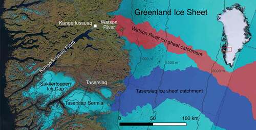
Figure 2. Average June–July–August air temperature recorded in Kangerlussuaq. The solid and dotted grey lines illustrate the 1949–2017 period average and standard deviation, respectively. Solid black lines give decadal averages. The ranking of the ten highest values is indicated at the top of the figure

To provide a better temporal context for the recent (2006–2017) observations of Watson River discharge and Greenland Ice Sheet studies dependent on these data, the primary aim of our study is to reconstruct a multi-decadal discharge record of the Watson River at annual time resolution using in situ observations. We use two other measurement records to reconstruct past discharge: (1) 1976–2014 discharge from Tasersiaq lake, draining a nearby ice-sheet catchment, and (2) 1949–2017 air temperature at Kangerlussuaq (Figure 2). Using the resulting 1949–2017 reconstruction, we contextualize Watson River discharge by quantifying recent increases and use the 2006–2017 observations to determine the characteristics of especially high-discharge years. Finally, we compare the reconstructed record with 1958–2016 runoff from the ice sheet and proglacial area, calculated by a downscaled version of the regional climate model RACMO2.

Study area

The Watson River is located in southern west Greenland, where its branches run for 26–33 km from the ice-sheet margin to its single outlet into the fjord at the Kangerlussuaq settlement (Figure 1). The river drains an approximately 12,000 km² sector (Lindbäck et al. 2015), or 0.7 percent of the Greenland Ice Sheet, and an approximately twenty times smaller (~590 km²) proglacial area (Hasholt et al. 2013). The river monitoring site is located just north of the Arctic Circle at 67.01°N by 50.68°W (10–20 m above sea level), and is well suited for discharge studies, because ice-sheet meltwater runoff variability is not dampened by passage through large proglacial lakes. Whereas the Watson River mostly runs over sediment planes, the monitoring site exhibits stable bedrock, guaranteeing a constant cross section, except in early spring (at low discharge) as a result of winter-accumulated ice.

The 1949–2017 average temperature recorded at Kangerlussuaq is −5.0°C. June-July-August (JJA) average temperature is well above freezing at nearly 10°C. Figure 2 shows that eight out of the ten warmest summers in Kangerlussuaq in the 1949–2017 period occurred since 2000, with both the 2000s and 2010s exceeding the long-term average by roughly one standard deviation. In contrast, some of the coldest summers are associated with preceding volcanic eruptions (Mernild et al. 2014), most notably El Chichón in 1982 (~6,300 km distance) and Mount Pinatubo in 1991 (~10,900 km distance; Abdalati and Steffen 1997).

The local climate is arid—the result of orographic shielding by the nearly 2 km tall Maniitsoq (Sukkertoppen) ice cap immediately southern west—with 1976–2016 annual average precipitation of 156 mm observed at Kangerlussuaq. Integrating this precipitation value over the proglacial area of the Watson River catchment (neglecting evapotranspiration) gives an annual contribution to discharge on the order of 0.1 km³, which is small in low-discharge years (e.g., 3.8 ± 0.6 km³ in 2015; Table 1) and negligible in peak-discharge years (e.g., 11.2 ± 1.7 km³ in 2010; Table 1), especially considering that precipitation likely reduces eastward of the meteorological measurement site at Kangerlussuaq. The regional climate model RACMO2 (Noël et al. 2017) confirms a small annual proglacial contribution to total discharge estimated at 2.6 ± 0.5 percent. With liquid precipitation values quickly diminishing with elevation on the ice sheet, we suggest that nearly all of the annual discharge through the Watson River is generated by the melting of snow and ice at the ice-sheet surface.

Table 1. Watson River discharge statistics for the 2006–2017 observational period. Values in brackets list rankings. Bold text signifies a top-three ranking

Year	Annual Total Discharge and Uncertainty (km^3)	Peak Discharge and Uncertainty (×10^3 m^3 s^−1), Excluding Jökullaups	Number of Days with Average Discharge over 200 m^3 s^−1	Number of Days with Average Discharge over 200 m^3 s^−1 and over the 2006–2017 Average (Black Line in Figure 5)
2006	5.4 ± 2.9 (8)	1.69 ± 1.19 (6)*	79 (8)	25 (7)
2007	7.5 ± 1.2 (5)	1.99 ± 0.30 (4)	87 (7)	57 (5)
2008	5.5 ± 0.9 (7)	1.29 ± 0.19 (10)	79 (8)	19 (8)
2009	4.9 ± 0.9 (9)	1.43 ± 0.21 (9)	94 (3)	18 (9)
2010	11.2 ± 1.7 (1)	2.38 ± 0.36 (2)	112 (1)	112 (1)
2011	7.8 ± 1.2 (4)	1.94 ± 0.29 (5)	89 (6)	67 (4)
2012	10.7 ± 1.6 (2)	3.22 ± 0.48 (1)	98 (2)	78 (2)
2013	4.3 ± 0.7 (10)	1.44 ± 0.22 (8)	71 (12)	10 (10)
2014	6.8 ± 1.0 (6)	1.59 ± 0.24 (7)	92 (5)	47 (6)
2015	3.8 ± 0.6 (12)	1.18 ± 0.18 (12)	73 (11)	10 (10)
2016	8.2 ± 1.3 (3)	2.19 ± 0.33 (3)	94 (3)	78 (2)
2017	4.3 ± 0.6 (11)	1.24 ± 0.19 (11)	79 (8)	6 (12)

*2006 peak discharge was not measured, but was estimated from air temperature (van As et al. 2017).

Figure 3. (A) Annual totals of Watson River discharge plotted against Tasersiaq discharge. (B) Annual totals of Watson River discharge plotted against annual sums of T^3.4, where T is daily average temperature (above freezing) recorded in Kangerlussuaq. Black dots represent Watson River measurements, and red dots are discharge values reconstructed from the Tasersiaq time series. (C) same as (B), but with temperature T_* calculated as the average between daily maximum and minimum temperature. Uncertainty ranges are indicated by error bars. Solid lines represent the best linear fits, and the dashed lines give the root-mean-square error. Discharge values for 2010 and 2012 are labeled with 10 and 12, respectively

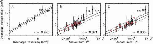
Figure 4. Annual totals of Watson River discharge from direct observations (black), and reconstructed from Tasersiaq discharge (red) and Kangerlussuaq air temperature (blue). The solid and dotted black lines illustrate the 1949–2000 average value and corresponding double standard deviations. Grey lines give the average and double standard deviations for 2001–2017. The ranking of the ten highest values is indicated at the top of the figure. The reconstructed time series of Greenland Ice Sheet meltwater discharge through the Watson River is provided in the supplementary material

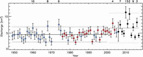
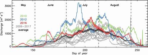
Figure 5. Hourly values of Watson River discharge for May–September 2006–2017 in grey with high-discharge years 2010, 2012, and 2016 plotted in color. The black line gives the 2006–2017 average. September peaks are the result of ice-dammed lake jökullaups

Our primary proxy to reconstruct Watson River discharge is discharge from the outlet of Tasersiaq, an approximately 65 km long and 2 km wide lake 90 km south of the Watson River (Figure 1). Tasersiaq had an annual average discharge of 2.6 km³ in the 1976–2014 period (data are available on request from Asiaq, the Greenland Survey). Ahlstrøm et al. (2017) estimate that a dominant portion (93%) of lake discharge is glacial runoff. The Tasersiaq ice-sheet catchment illustrated in Figure 1 is delineated by Lindbäck et al. (2015), but its area is exaggerated compared to the more realistic delineation by Ahlstrøm et al. (2017), who report a contributing ice area of approximately 7,000 km². Including the runoff from the steep slopes of the Tasersiaq Sermia ice cap directly south of the lake, the Tasersiaq ice-covered catchment is more than half the size of the Watson River ice-sheet catchment. The Tasersiaq ice-sheet catchment is roughly 50 percent wider in the ablation area, from where most meltwater originates, but the Watson River catchment has a markedly gentler slope and reaches elevations well below 1,000 m above sea level, and therefore generally has a more productive melt area (Figure 1). Measurements of air temperature at the Tasersiaq hydrometric station reveal that at an elevation of approximately 690 m above sea level the local above-freezing temperatures are generally 3–5°C below those at Kangerlussuaq. The catchment’s location directly on the lee side of tall ice caps yields annual precipitation values comparable to those at Kangerlussuaq, estimated at 161 mm by Ahlstrøm et al. (2017).

Methods

Watson River discharge is monitored approximately 25 km from the Greenland Ice Sheet margin, 150 m upstream of the bridge in the Kangerlussuaq settlement in southern west Greenland (Figure 1). The measurement infrastructure was established in 2006 and was maintained by the University of Copenhagen, Department of Geosciences and Natural Resource Management until 2013 (Hasholt et al. 2013). Thereafter, the Geological Survey of Denmark and Greenland continued the monitoring as part of the Programme for Monitoring of the Greenland Ice Sheet (data available at www.PROMICE.dk). Water stage is measured and converted to hourly averages of discharge using a stage-discharge relation largely determined by acoustic Doppler current profiling (van As et al. 2017). Uncertainty was chosen to be a conservative 15 percent, except for 2006, when a substantial data gap occurred, leading to a 53 percent uncertainty. For a detailed description of the Watson River monitoring methodology we refer to van As et al. (2017). In this study we focus on the annual discharge totals for the 2006–2017 period. To extend the data record back in time, we apply two methods.

First, we use annual discharge totals derived from stage measurements taken at the outlet of Tasersiaq lake (Figure 1). Similar to the Watson River, Tasersiaq receives the bulk (93%) of its water from ice-sheet runoff (Ahlstrøm et al. 2017). The measurement principle at both sites is identical. Tasersiaq stage is recorded at a three-hour temporal resolution (daily before 1979) and dates back to 1975. For further details on Tasersiaq monitoring and data coverage we refer to Ahlstrøm et al. (2017). Despite data gaps prohibiting the calculation of some annual totals, the dataset supplies us with thirty-two annual values for the thirty-nine-year time span (1976–2014) of the data record, twenty more than the Watson River record. The eight years (2007–2014) that both time series overlap reveal a high (r = 0.97, p < 10^–4) correlation in discharge from the two nearby catchments. The high correlation is partly the result of the large (factor-three) range in annual discharge totals in the 2007–2014 period (Figure 3A). We argue that this high correlation allows Tasersiaq and Watson River discharges to be reciprocal predictors. We therefore use linear regression, taking into account measurement uncertainties, to derive the fit parameters describing Watson River annual discharge (Q) as a function of Tasersiaq annual discharge (Q_Watson = 1.45 × Q_Tasersiaq + 1.6; Figure 3A). We find a root-mean-square error (RMSE) of 0.56 km³ (8% of the eight-year average) between the original and reconstructed Watson River time series, and consider this an additional uncertainty encompassing regional differences and Tasersiaq measurement error. We add this RMSE value to the Watson River discharge uncertainty for reconstructed values through standard (quadratic) addition. Including annual discharge totals reconstructed from Tasersiaq measurements provides us with thirty-six annual values of Watson River discharge within the 1976–2017 period.

To derive values for the six missing years for the 1976–2017 period and to extend the time series even further back, we use air temperature recorded in Kangerlussuaq since 1949 as our secondary proxy. Until 1970, measurements of daily maximum and minimum temperature were taken by the U.S. military, available from https://www.ncdc.noaa.gov. Since 1973, the Danish Meteorological Institute (DMI) has been conducting the measurements at three-hourly (1973–1998) and hourly (1998–present) time resolutions (Cappelen 2017; data are accessible through http://www.dmi.dk). Local melting, and thus glacial meltwater runoff, can be approximated using a linear temperature-index model. van As et al. (2017) show that meltwater runoff from the entire Watson River catchment can be estimated using a power law, in which Kangerlussuaq air temperature predicts Watson River discharge: Q = C × T^3.4, where T is temperature above freezing and C is a constant. For the DMI measurements since 1973, we calculate daily average temperatures to homogenize the time series and use them to calculate annual sums of T^3.4. The two time series correlate at r = 0.87 (p ≪ 10^–4). We then use the parameters of the best linear fit to derive missing annual discharge totals for the period with complete annual coverage of daily average temperatures; that is, since 1974. Only for 2012 does the regression fall short of the observed value beyond uncertainty. This is likely because of a combination of factors, such as the upward migration of the ice-sheet runoff limit (Mikkelsen et al. 2016), reduced springtime refreezing due to below-average winter snow accumulation (Tedesco et al. 2013), and melt enhancement through a melt-albedo feedback (Box et al. 2012). This part of the temperature-based reconstruction adds another eight annual values, resulting in a continuous forty-four-year (1974–2017) record of Watson River discharge.

For earlier years, when only daily maximum and minimum temperature were measured, we repeat the above exercise, but calculate a daily temperature T_* by averaging daily maximum and minimum temperature (n.b.: not daily average temperature). We do not calculate daily average temperatures from the maxima and minima following, for example, Dall’Amico and Hornsteiner (2006). Using T_* for linear regression with discharge is justified by the high correlation of 0.89 (p ≪ 10^–4) in Figure 3C (n = 33), even marginally higher than for T in Figure 3B (n = 36). Using the 1949–1970 Kangerlussuaq temperatures adds twenty-one years to the discharge reconstruction, giving a total of sixty-five annual values for the 1949–2017 (sixty-nine-year) period. Owing to an incomplete meteorological record, values for 1951 and 1971–1973 cannot be reconstructed.

The RMSE values separating temperature-reconstructed discharge and Watson River discharge (including Tasersiaq-reconstructed values) absorb uncertainty from interannual variability in precipitation, solar radiation, and other factors impacting annual discharge that are not well represented by the power-law temperature dependency of Watson River discharge. We again assume that the uncertainties are independent and random, and combine these RMSEs through standard (quadratic) error addition to the Watson River and Tasersiaq-derived discharge uncertainty to obtain an uncertainty estimate for the temperature-derived discharge values. Note that reconstructed values can have smaller absolute uncertainties than measured ones, because Watson River measurement uncertainty is expressed as a fraction of the annual total. The reconstructed time series of Greenland Ice Sheet meltwater discharge through the Watson River is provided in the supplementary material.

Results

Analysis of the 1949–2017 discharge record

The reconstructed Watson River discharge time series consists of sixty-five annual totals within the 1949–2017 period (Figure 4), making it the longest annual time series of Greenland Ice Sheet melting, assuming negligible contributions from the proglacial area. The 1949–2017 average ice-sheet meltwater discharge through the Watson River is estimated to be 5.0 km³ per year, with a minimum value of 2.2 km³ for 1983 and a maximum value of 11.2 km³ for 2010. Interannual variability measured by the 1949–2017 standard deviation is 1.8 km³, or 35 percent of the average. Consistent with the high summer temperatures in Greenland throughout the past two decades (e.g., Figure 2), Figure 4 illustrates that discharge since the turn of the century has been anomalously high in a multi-decadal context, also when not taking into account the temperature-based part of the reconstruction (the blue dots in Figure 4). While for 1949–2000 we find Watson River discharge to average 4.6 km³ with a standard deviation of 1.1 km³ (25% of the average), average meltwater production has increased to 6.5 km³ with a standard deviation of 2.2 km³ (34% of the average) for 2001–2017. The 1.9 km³ (42%) increase in the average exceeds one standard deviation of the 1949–2000 average. Comparing 2003–2017 (6.7 ± 2.3 km³) to 1949–2002, the increase is even larger at 46 percent.

The increase in interannual variability is larger than the increase in discharge volume, expressed through changes in standard deviation. Since 2001 the standard deviation increased increased by 97% from 1.1 km³ to 2.2 km³, and since 2003 by 112 percent compared to the 1949–2002 period. Larger interannual variability is to be expected with increasing annual average values, but variability likely changes disproportionally in our study area because of a number of melt amplifiers known to be at play in recent years, driven by atmospheric circulation anomalies (Fettweis et al. 2013; McLeod and Mote 2016; Rajewicz and Marshall 2014). In response to atmospheric forcing, the ice-sheet surface has darkened, enhancing melting through melt-albedo feedback (Box et al. 2012; Tedesco et al. 2013). Further, firn densification of the ice-sheet accumulation area has also been observed; formation of thick ice layers renders porous firn inaccessible for meltwater retention, promoting runoff (De La Peña et al. 2015; Machguth et al. 2016). Both the ice-sheet darkening and runoff line elevation increase are in part a result of an observed gradual increase in equilibrium line altitude (where annual SMB = 0) in the Kangerlussuaq region (Smeets et al. 2018). Also, meltwater runoff is amplified by the ice sheet’s hypsometry because increases in atmospheric temperature yield exponential increases in melt area (Mikkelsen et al. 2016; van As et al. 2017).

The increase in discharge in recent decades led to the occurrence of the five top-ranking discharge years (or, seven out of ten) since 2003 (Figure 4). Especially the years 2010 and 2012 show large positive excursions. The three largest discharge years in our record are 2010, 2012, and 2016 (Table 1), and they occurred within the period of monitoring at the Watson River bridge site, allowing us to investigate how these years came to be record setting. For instance, 2016 (ranked third) was marked by an early start to the melt season in mid-May (Figure 5), and included six distinct periods in which the ice sheet in the Kangerlussuaq region released above-average discharge volumes (not counting the discharge spike as a result of a jökullaup that occurred the second week of September). In 2012 (ranked second), the two single largest discharge peaks on record took place (Figure 5), the first of which washed out the road dam at the Kangerlussuaq bridge, constructed nearly six decades before in 1955 (Mikkelsen et al. 2016). In 2010 (ranked first), discharge exceeded the 2006–2017 average throughout the entire melt season, with melting already well underway in early May and with discharge values of up to 1,400 m³ s^–1 recorded as late as September. Table 1 shows that several characteristics are shared by peak discharge years: (1) discharge peaks exceeding 2,000 m³ s⁻¹ in mid-summer; (2) a long melt season, with relatively high discharge starting in May and lasting well into September; and (3) above-average discharge values throughout most of the melt season.

These three features of peak discharge years cannot be considered independent of the high atmospheric temperatures in Greenland in recent years (Figure 2) during a phase with distinctly negative North Atlantic Oscillation (NAO) values favoring northward advection of warm, dry air (e.g., Fettweis et al. 2013). For instance, air temperatures during 2016 were abnormally high with record-setting spring-average temperatures measured at Kangerlussuaq (6.7°C above the 1981–2010 average), Aasiaat (+6.0°C), and Summit (+4.8°C), and record summer temperatures at east and south Greenland measurement sites such as Danmarkhavn (+2.3°C), Tasiilaq (+2.3°C), and Narsarsuaq (+1.7°C; Tedesco et al. 2016). The summer (JJA) 2012 average temperatures were record setting at multiple sites along the Greenland west coast, and in 2010 both the winter and spring average temperatures are yet to be surpassed for the entire southern west (Cappelen 2017).

Only in three years since 2000 is discharge found to be below the 1949–2000 average, namely in 2013 (ranking twenty-fifth lowest of sixty-five annual totals), 2015 (seventeenth), and 2017 (twenty-second), when discharge was about half that of high-discharge years. In contrast to the high-discharge years, 2013, 2015, and 2017 rank low or lowest in terms of peak discharge and length of the melt season within our 2006–2017 observational period (Table 1). In our reconstruction, the lowest annual discharge values are roughly four times smaller than the 2010 and 2012 values. Of the ten lowest annual discharge values, seven are a direct consequence of our temperature-based methodology. The three other low-ranking discharge years are 1983 (lowest), 1992 (fourth), and 1996 (seventh), and these values are based on (low) discharge monitored at Tasersiaq (Figure 4). Yet these three years are also associated with low summer temperatures (Figure 2). For 1983 and 1992, the low temperatures are probably partly the result of major volcanic eruptions in the preceding year—respectively, El Chichón in Mexico and Mount Pinatubo in the Phillipines (Abdalati and Steffen 1997)—effectively halving annual discharge compared to the 1949–2000 norm (Figure 4). The ashes injected into the atmosphere during major volcanic eruptions reflect solar radiation, lowering temperatures on a global scale for a limited (~1 y) time period. Figures 2 and 4 suggest that the cooling effect of the early 1963 eruption of Mount Agung in Indonesia was also noticeable in Greenland runoff (Mernild et al. 2014).

For the 2006–2017 period, we find high correlation between annual discharge and the other columns in Table 1: peak discharge (r = 0.92, excluding 2006 when peak discharge was not captured), the number of days with average discharge exceeding a low threshold of 200 m³ s⁻¹ (r = 0.87), and the number of days with discharge also exceeding the 2006–2017 average (r = 0.97). These high correlation values suggest skill in estimating peak discharge and (high) discharge-period length from reconstructed annual discharge for the 1949–2005 period (Figure 4), which can be of use to studies of, for example, hydropower potential.

Multi-Decadal discharge as a model evaluation tool

A benefit of our ice-sheet discharge reconstruction spanning a period of sixty-nine years is its application as an evaluation tool for runoff calculations by models that calculate surface mass balance. To illustrate, we compare reconstructed Watson River discharge to runoff from primarily melting and liquid precipitation calculated by the regional climate model RACMO2 (for details see Noël et al. 2017). The model includes all of Greenland in its domain, and is run for 1958–2016 at 11 km horizontal resolution is subsequently downscaled to 1 km (Noël et al. 2017). For the present study, runoff to the Watson River was integrated over the approximately 12,000 km² ice-sheet catchment characterized by Lindbäck et al. (2015; Figure 1), and terrestrial runoff to the Watson River was integrated over the approximately 590 km² proglacial catchment delineated by Hasholt et al. (2013). The model is forced by reanalysis data at remote lateral boundaries well off the Greenland coast, and thus is not fed by weather-station measurements such as those used for our discharge reconstruction.

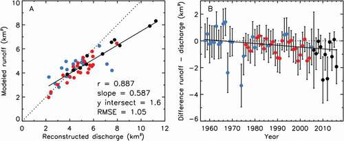
The correlation between reconstructed discharge and modeled runoff is high (r = 0.89, p ≪ 10^–4), suggesting that interannual runoff variability is well captured by RACMO2. Indeed, compared to methodology using satellite observations of sediment plumes in the Kangerlussuaq fjord, RACMO2 proves to be superior: annual plume-based values by McGrath et al. (2010) for 2001–2008 correlate at r = 0.44 with reconstructed Watson River discharge, where RACMO2 values correlate at r = 0.90 for the same period.

However, Figure 6A reveals an underestimation of more than 20 percent for RACMO2 peak values. The average bias is near-zero for the 1960s (Figure 6B), for which period our discharge values are reconstructed from air temperature. The bias grows by an average of −1.4 × 10⁻² km³ yr⁻¹ in the 1980s, before Watson River discharge had increased (Figure 4). The developing underestimation of RACMO2 values is virtually identical regardless of whether temperature-reconstructed discharge is included. The time dependency of the bias raises the question of whether regional climate models are currently capable of fully capturing the magnitude of runoff increase in projections in a warm future climate. Based on our comparison, there appears to be a significant potential for future ice-sheet runoff, and thus subsequent sea-level rise, to be underestimated.

Figure 6. (A) Annual totals of 1958–2016 RACMO2-modeled freshwater runoff from the Kangerlussuaq ice sheet and proglacial catchment plotted against reconstructed Watson River discharge. The dotted line illustrates the 1:1 relation. (B) Difference between ice-sheet runoff and river discharge. Error bars give the Watson River reconstructed discharge uncertainty. Solid lines represent the best linear fits. For color coding, see Figure 4

Model underestimation of ice-sheet melt resulting from underestimating nonradiative energy fluxes, especially during extreme events, has been reported by Fausto et al. (2016). Also, models can struggle to accurately calculate ice albedo, which exhibits a first-order control on surface melting. But other factors causing a bias, not related to the accuracy with which physical processes are captured, may be at play as well. For instance, the Lindbäck et al. (2015) ice-sheet catchment delineation could underestimate surface area at the upper runoff elevations, causing melting at these elevations not to contribute sufficiently to catchment-total runoff as melting migrates up-glacier. Underestimated catchment area at high elevation was also suggested as a potential issue by van As et al. (2017), but only for the largest of the melt events in the period 2010–2012. Another possibility is that Watson River discharge is overestimated despite strong efforts to constrain it and its uncertainty estimate. Yet van As et al. (2017) find that their observation-based annual ice-sheet runoff calculations match river discharge within uncertainty, without amplitude-dependent bias.

Two years are obvious outliers in the discharge comparison with RACMO2 (Figure 6B): 1968 and 1974, in which our reconstructed time series gives values more than two standard deviations above average (Figure 4), while RACMO2 suggests near-average values well beyond the Watson River uncertainty range (Figure 6B). Sisimiut (~130 km due west) measurements confirm that the 1974 spring and summer were warmer than average (Cappelen 2017). In 1968, sizeable positive temperature anomalies occurred in April and May both at Kangerlussuaq and Sisimiut (not contributing to the June–August average plotted in Figure 2). It is plausible that relatively high spring temperatures such as in 1968 and 1974 do not yield the same impact on ice-sheet runoff as in summer, because in spring the lower ablation area is covered by snow as opposed to bare ice in summer. Alternatively, high wintertime accumulation can in spring result in relatively high refreezing rates and thus reduced runoff. However, RACMO2 calculates that 1968 and 1974 rank among the five years with the lowest accumulation in the Kangerlussuaq ice-sheet catchment in the fifty-nine-year model period, suggesting that interannual variability in accumulation does not exert a dominant control on meltwater discharge in the arid Kangerlussuaq region. If the 1968 and 1974 discharge values are indeed overestimated in our reconstruction, ranking eighth and sixth highest, respectively (Figure 4), the Watson River discharge increase since the turn of the century is even more substantial than reported here.

Conclusions

The Watson River in southern west Greenland drains glacial meltwater from a large, approximately 12,000 km² ice-sheet catchment. To be able to interpret the discharge monitored since 2006 on multi-decadal (climatic) time scales, we reconstructed annual discharge values for the 1949–2017 period using observational records of Tasersiaq lake discharge and Kangerlussuaq air temperature. Watson River discharge is shown to have been exceptionally large in the current century. The 2003–2017 average discharge exceeded the 1949–2002 average by 46 percent. At the same time, interannual variability of meltwater discharge increased by 112 percent. We speculate that the observed changes cannot just be the result of atmospheric forcing, but require melt/runoff amplification by melt-albedo feedback; by ice-layer formation, reducing the refreezing potential in the accumulation area; and by ice-sheet hypsometry, increasing melt area exponentially with rising temperature.

The largest discharge years since 1949 are 2010 (first), 2012 (second), and 2016 (third). High-discharge years are the result not only of more intense ice-sheet melting but also of a prolonged melt season. High discharge years are commonly associated with relatively warm conditions during the melt season, also for years in which our values are not reconstructed from air temperature. Several of the lowest-discharge years followed major volcanic eruptions, which lowered atmospheric temperatures globally and thereby roughly halved meltwater runoff from the Greenland Ice Sheet.

The 1949–2017 reconstruction of Watson River discharge clearly reveals the impact of climate variability on the Greenland Ice Sheet mass balance. The long-time series offers a rare opportunity to evaluate models that calculate Greenland Ice Sheet surface mass balance and runoff. For instance, comparison to discharge calculated by a downscaled version of the RACMO2 regional climate model suggests that a model bias develops with time and/or climate warming. The increasing bias could imply that future ice-sheet mass loss calculated by regional climate models currently is underestimated.

Acknowledgments

We thank Ken Mankoff for his help and three reviewers for constructive comments. This is a PROMICE publication.

Additional information

Funding

Over the years, Watson River discharge monitoring has been (co)financed through various funding sources: the Commission for Scientific Research in Greenland, the Danish Natural Science Research Council, the Center for Permafrost (CENPERM), the Department of Geosciences and Natural Resource Management (IGN), the Greenland Analogue Project (GAP), and the Danish Energy Agency’s (ENS) DANCEA program. We acknowledge support in Kangerlussuaq by the Centre for Ice and Climate (CIC/NBI), CH2M HILL Polar Services (CPSpolar), Kangerlussuaq International Science Support (KISS), and the Greenland Survey (Asiaq). BPYN and MRvdB acknowledge funding from the Polar Program of the Netherlands Organization for Scientific Research (NWO/NPP) and the Netherlands Earth System Science Center (NESSC).

References

- Abdalati, W., and K. Steffen. 1997. The apparent effects of the Mt. Pinatubo eruption on the Greenland ice sheet melt extent. Geophysical Research Letters 24 (14):1–10.
- Ahlstrøm, A. P., D. Petersen, P. L. Langen, M. Citterio, and J. E. Box. 2017. Abrupt shift in the observed runoff from the southwestern Greenland ice sheet. Science Advances 3 (12):e1701169. doi:https://doi.org/10.1126/sciadv.1701169.
- Bendixen, M., L. L. Iversen, A. A. Bjørk, B. Elberling, A. Westergaard-Nielsen, I. Overeem, K. Barnhart, S. A. Khan, J. E. Box, J. Abermann, K. Langley, and A. Kroon. 2017. Delta progradation in Greenland driven by increasing glacial mass loss. Nature. doi:https://doi.org/10.1038/nature23873.
- Box, J. E., X. Fettweis, J. C. Stroeve, M. Tedesco, D. K. Hall, and K. Steffen. 2012. Greenland ice sheet albedo feedback: Thermodynamics and atmospheric drivers. The Cryosphere 6:821−839. doi:https://doi.org/10.5194/tc-6-821-2012.
- Cappelen, J., ed. 2017. Weather observations from Greenland 1958-2016 - Observation data with description. Danish Meteorological Institute Report 17-08:31.
- Chandler, D. M., J. L. Wadham, G. P. Lis, T. Cowton, A. Sole, I. Bartholomew, J. Telling, P. Nienow, E. B. Bagshaw, D. Mair, S. Vinen, and A. Hubbard. 2013. Evolution of the subglacial drainage system beneath the Greenland Ice Sheet revealed by tracers. Nature Geoscience 6:195–98. doi:https://doi.org/10.1038/ngeo1737.
- Dall’Amico, M., and M. Hornsteiner. 2006. A simple method for estimating daily and monthly mean temperatures from daily minima and maxima. International Journal of Climatology 26:1929–36. doi:https://doi.org/10.1002/joc.1363.
- De La Peña, S., I. M. Howat, P. W. Nienow, M. R. van den Broeke, E. Mosley-Thompson, S. F. Price, D. Mair, B. Noël, and A. J. Sole. 2015. Changes in the firn structure of the western Greenland Ice Sheet caused by recent warming. The Cryosphere 9:1203–11. doi:https://doi.org/10.5194/tc-9-1203-2015.
- Doyle, S. H., A. Hubbard, R. S. W. van de Wal, J. E. Box, D. van As, K. Scharrer, T. W. Meierbachtol, P. C. J. P. Smeets, J. T. Harper, E. Johansson, R. H. Mottram, A. B. Mikkelsen, F. Wilhelms, H. Patton, P. Christoffersen, and B. Hubbard. 2015. Amplified melt and flow of the Greenland ice sheet driven by late-summer cyclonic rainfall. Nature Geoscience 8:647–53. doi:https://doi.org/10.1038/ngeo2482.
- Fausto, R. S., D. van As, J. E. Box, W. Colgan, P. L. Langen, and R. H. Mottram. 2016. The implication of non-radiative energy fluxes dominating Greenland exceptional surface melt in 2012. Geophysical Research Letters 43. doi:https://doi.org/10.1002/2016GL067720.
- Fettweis, X., E. Hanna, C. Lang, A. Belleflamme, M. Erpicum, and M. Gallée. 2013. Brief communication “Important role of the mid-tropospheric atmospheric circulation in the recent surface melt increase over the Greenland ice sheet”. The Cryosphere 7:241–48. doi:https://doi.org/10.5194/tc-7-241-2013.
- Fitzpatrick, A. A. W., A. L. Hubbard, J. E. Box, D. J. Quincey, D. van As, A. P. B. Mikkelsen, S. H. Doyle, C. F. Dow, B. Hasholt, and G. A. Jones. 2014. A decade (2002–2012) of supraglacial lake volume estimates across Russell Glacier, West Greenland. The Cryosphere 8:107–21. doi:https://doi.org/10.5194/tc-8-107-2014.
- Hasholt, B., A. B. Mikkelsen, M. H. Nielsen, and M. A. D. Larsen. 2013. Observations of runoff and sediment and dissolved loads from the Greenland ice sheet at Kangerlussuaq, West Greenland, 2007 to 2010. Zeitschrift Für Geomorphologie 57:3–27.
- Langen, P. L., R. H. Mottram, J. H. Christensen, F. Boberg, C. B. Rodehacke, M. Stendel, D. van As, A. P. Ahlstrøm, J. Mortensen, S. Rysgaard, D. Petersen, K. H. Svendsen, G. Aðalgeirsdóttir, and J. Cappelen. 2015. Quantifying energy and mass fluxes controlling Godthåbsfjord freshwater input in a 5 km simulation (1991-2012). Journal of Climate 28:3694–713. doi:https://doi.org/10.1175/JCLI-D-14-00271.1.
- Lindbäck, K., R. Pettersson, A. L. Hubbard, S. H. Doyle, D. van As, A. B. Mikkelsen, and A. A. Fitzpatrick. 2015. Subglacial water drainage, storage, and piracy beneath the Greenland Ice Sheet. Geophysical Research Letters 42 (18):7606–14. doi:https://doi.org/10.1002/2015GL065393.
- Machguth, H., M. MacFerrin, D. van As, J. E. Box, C. Charalampidis, W. Colgan, R. S. Fausto, H. A. J. Meijer, E. Mosley-Thompson, and R. S. W. van de Wal. 2016. Greenland meltwater storage in firn limited by near-surface ice formation. Nature Climate Change 6:390–93. doi:https://doi.org/10.1038/nclimate2899.
- McGrath, D., K. Steffen, I. Overeem, S. Mernild, B. Hasholt, and M. van den Broeke. 2010. Sediment plumes as a proxy for local ice-sheet runoff in Kangerlussuaq Fjord, West Greenland. Journal of Glaciology 56 (199):813–21. doi:https://doi.org/10.3189/002214310794457227.
- McLeod, J. T., and T. L. Mote. 2016. Linking interannual variability in extreme Greenland blocking episodes to the recent increase in summer melting across the Greenland ice sheet. International Journal of Climatology 36:1484–99. doi:https://doi.org/10.1002/joc.4440.
- Mernild, S. H., E. Hanna, J. C. Yde, J. Cappelen, and J. K. Malmros. 2014. Coastal Greenland air temperature extremes and trends 1890-2010: Annual and monthly analysis. International Journal of Climatology 34:1472–87. doi:https://doi.org/10.1002/joc.3777.
- Mikkelsen, A. B., A. Hubbard, M. MacFerrin, J. E. Box, S. H. Doyle, A. Fitzpatrick, B. Hasholt, H. L. Bailey, K. Lindbäck, and R. Pettersson. 2016. Extraordinary runoff from the Greenland ice sheet in 2012 amplified by hypsometry and depleted firn retention. The Cryosphere 10:1147–59. doi:https://doi.org/10.5194/tc-10-1147-2016.
- Noël, B., W. J. van de Berg, J. M. van Wessem, E. van Meijgaard, D. van As, J. T. M. Lenaerts, S. Lhermitte, P. Kuipers Munneke, C. J. P. P. Smeets, L. H. van Ulft, R. S. W. van de Wal, and M. R. van den Broeke. 2017. Modelling the climate and surface mass balance of polar ice sheets using RACMO2, Part 1: Greenland (1958-2016). The Cryosphere Discussions. doi:https://doi.org/10.5194/tc-2017-201.
- Overeem, I., B. Hudson, E. Welty, A. Mikkelsen, J. Bamber, D. Petersen, A. Lewinter, and B. Hasholt. 2015. River inundation suggests ice-sheet runoff retention. Journal of Glaciology 61:776–88. doi:https://doi.org/10.3189/2015JoG15J012.
- Rajewicz, J., and S. J. Marshall. 2014. Variability and trends in anticyclonic circulation over the Greenland ice sheet, 1948-2013. Geophysical Research Letters 41:2842–50. doi:https://doi.org/10.1002/2014GL059255.
- Rennermalm, A. K., L. C. Smith, V. W. Chu, J. E. Box, R. R. Forster, M. R. van den Broeke, D. van As, and S. E. Moustafa. 2013. Evidence of meltwater retention within the Greenland ice sheet. The Cryosphere 7:1433–45. doi:https://doi.org/10.5194/tc-7-1433-2013.
- Smeets, C. J. P. P., P. Kuipers Munneke, D. van As, M. R. van den Broeke, W. Boot, J. Oerlemans, H. Snellen, C. H. Reijmer, and R. S. W. van de Wal. 2018. The K-transect in west Greenland: Twenty-three years of weather station data. Arctic, Antarctic, and Alpine Research 50. doi: https://doi.org/10.1080/15230430.2017.1420954.
- Smith, L. C., V. W. Chu, K. Yang, C. J. Gleason, L. H. Pitcher, A. K. Rennermalm, C. J. Legleiter, A. E. Behar, B. T. Overstreet, S. E. Moustafa, M. Tedesco, R. R. Forster, A. L. LeWinter, D. C. Finnegan, Y. Sheng, and J. Balog. 2015. Efficient meltwater drainage through supraglacial streams and rivers on the south-west Greenland ice sheet. Proceedings of the National Academy of Sciences 112:1001–06. doi:https://doi.org/10.1073/pnas.1413024112.
- Tedesco, M., J. E. Box, J. Cappelen, R. S. Fausto, X. Fettweis, T. Mote, C. J. P. P. Smeets, D. van As, I. Velicogna, R. S. W. van de Wal, and J. Wahr. 2016. 2016: Greenland Ice Sheet [in Arctic Report Card 2016], http://www.arctic.noaa.gov/Report-Card.
- Tedesco, M., X. Fettweis, T. Mote, J. Wahr, P. Alexander, J. E. Box, and B. Wouters. 2013. Evidence and analysis of 2012 Greenland records from spaceborne observations, a regional climate model and reanalysis data. The Cryosphere 7:615–30. doi:https://doi.org/10.5194/tc-7-615-2013.
- van As, D., A. Bech Mikkelsen, M. Holtegaard Nielsen, J. E. Box, L. Claesson Liljedahl, K. Lindbäck, L. Pitcher, and B. Hasholt. 2017. Hypsometric amplification and routing moderation of Greenland ice sheet meltwater release. The Cryosphere 11:1371–86. doi:https://doi.org/10.5194/tc-11-1371-2017.
- van den Broeke, M. R., E. M. Enderlin, I. M. Howat, P. Kuipers Munneke, B. P. Y. Noël, W. J. van de Berg, E. van Meijgaard, and B. Wouters. 2016. On the recent contribution of the Greenland ice sheet to sea level change. The Cryosphere 10:1933–46. doi:https://doi.org/10.5194/tc-10-1933-2016.