Combined effects of early snowmelt and climate warming on mountain lake temperatures and fish energetics

ABSTRACT

Mountain regions are experiencing some of the highest air temperature increases and ice cover decreases. However, few studies have examined the effects of climate warming and earlier snowmelt on mountain lake thermal characteristics and energetic implications for fish. We assessed potential climate-induced thermal changes and energetic consequences for cutthroat trout (Oncorhynchus clarkii spp.) and brook trout (Salvelinus fontinalis) in the Southern Rocky Mountains, United States. We found that summer growing degree days increased by an average 21 percent with 2°C air warming and 43 percent with 5°C air warming. But earlier snowmelt increased growing degree days by an average 48 percent. The average maintenance ration with 2°C and 5°C warming increased respectively by 13.8 and 21.9 percent for cutthroat trout and 23.8 and 37.4 percent for brook trout. The average increase in food required with earlier snowmelt was 43.4 percent for cutthroat trout and 52.3 percent for brook trout. Thus, earlier snowmelt can have a greater effect on fish energy requirements than a 5°C rise in air temperatures. Snowmelt recession together with a 5°C air temperature rise could more than double food requirements for fish to maintain constant body weight. If lake productivity increases with these climatic changes, then trout growth could improve; otherwise, energetic demands may result in lower fish growth.

KEYWORDS:

• Climate change
• general lake model
• snowpack
• high elevation lakes
• cutthroat trout

Introduction

Effects of climate-induced variation in the magnitude and timing of snowmelt are well studied in lotic systems (e.g., Martinec 1975; Brubaker and Rango 1996; Yarnell, Viers, and Mount 2010), particularly in the western United States and other regions where rivers exhibit a snowmelt hydrograph (Poff and Ward 1990). Snowmelt can be an important contributor to stream flow, but it also buffers stream temperatures from atmospheric warming (Lisi et al. 2015). Reduced snowpack and earlier melting allow rivers to warm sooner, affecting phenology, energetic costs, and consumptive demand of lotic ectotherms like fishes (Railsback and Rose 1999; Lisi et al. 2015). These hydrologic effects on water temperature and physiology are compounded by rising air temperatures, which allow rivers to reach higher seasonal maxima (Wenger et al. 2011). Changes to snowmelt can also affect lakes with inflows, but much less is known about how lake temperatures and lacustrine biota respond to this component of climate change or how such hydrologic changes will interact with rising air temperatures.

Many studies have demonstrated that worldwide lakes are becoming warmer and more strongly stratified (Adrian et al. 2009; Kirillin 2010; Schmid, Hunziker, and Wüest 2014; O’Reilly et al. 2015; Michelutti et al. 2016; Christianson et al. 2019; Christianson, Johnson, and Hooten 2020). These changes to lake thermal regimes have important implications for lentic ecosystem structure and function. Warming raises metabolic rates of aquatic organisms and increases their oxygen and food requirements (Ficke, Myrick, and Hansen 2007). However, warming also reduces water column mixing, which can prolong stratification (Adrian et al. 2009; Woolway and Merchant 2019), lead to reduced oxygen availability (Jankowski et al. 2006), and segregate predators from their prey (Johnson, Pate, and Hansen 2017). Warming can also reduce the ability of lakes to sequester CO₂ (Yvon-Durocher et al. 2010), an important role of lakes in the global carbon cycle (Tranvik et al. 2009). Further, climate warming has decreased the duration of ice cover in temperate lakes (Magnuson et al. 2000; Dibike et al. 2011; Sharma et al. 2019). Together these effects are increasing growing season degree days and annual energetic demands for fish and other aquatic organisms (Roberts et al. 2017; Honsey, Venturelli, and Lester 2018). Thus, it is important to understand how various aspects of climate change are driving lake warming and stratification patterns.

Although the effects of climate change on lakes are ubiquitous, the magnitude of change in lake temperature and ice cover duration varies across regions and lake types (Magnuson et al. 2000; Luoto and Nevalainen 2013; O’Reilly et al. 2015; Christianson et al. 2019). For example, lakes at high elevation are experiencing greater air temperature rise (Pepin et al. 2015; Preston et al. 2016) and reductions in ice cover duration than their lower elevation counterparts (Thompson et al. 2005; Roberts et al. 2017). Given that high elevation lakes are usually colder and have longer ice-covered periods, and therefore shorter growing seasons than lakes at low elevation, climate-induced changes can have disproportionately large effects on high elevation lake thermal regimes. The duration of ice cover in high elevation lakes is closely linked to the processes that govern snowmelt dynamics (Magnuson et al. 2000; Preston et al. 2016; Sadro, Melack, Sickman, and Skeen 2018; Sadro, Sickman, Melack, and Skeen 2018). Low snowpack can result in earlier snowmelt (Yarnell, Viers, and Mount 2010; Musselman et al. 2017), which has been linked to shorter ice cover duration (Parker, Vinebrooke, and Schindler 2008; Preston et al. 2016) and higher summer temperatures (Sadro, Melack, Sickman, and Skeen 2018). Generally, across western North America, less precipitation has been falling as snow (Berg and Hall 2017), and annual snowpack has been declining (Fyfe et al. 2017). Partly as a result of reduced snowpack, snowmelt dates are retreating in many high elevation areas (Barnett, Adam, and Lettenmaier 2005; Mote et al. 2005; Musselman et al. 2017). Concomitantly, ice-off dates have shifted earlier, and open water duration has increased in high elevations lakes, including those in the Southern Rocky Mountains (SRM), United States (Preston et al. 2016; Roberts et al. 2017). However, relatively few studies have examined effects of altered snowmelt and ice cover dynamics on high elevation lake temperatures and the energetics implications for their biota, including fishes.

Historically, fish did not occur in most high elevation lakes of the western United States (Knapp 1996) but, because of a desire to create new sport fishing opportunities and habitat degradation and introduced species at lower elevations, managers transplanted both native and nonnative species of trout to most of the more remote, isolated, and relatively pristine lakes at higher elevations (Bahls 1992). Consequently, high elevation lakes in the region have become important refuge habitat for native coldwater species of conservation concern, such as cutthroat trout Oncorhynchus clarkii (Marnell, Behnke, and Allendorf 1987; Roberts et al. 2013). These lakes also continue to be popular with anglers seeking these fish as well as introduced species such as brook trout Salvelinus fontinalis (Meyer and Schill 2007). Though predicted increases in seasonal thermal maxima are not expected to exceed physiological optimum temperatures for these species (Bear, McMahon, and Zale 2007; Christianson, Johnson, and Hooten 2020), warmer and longer growing seasons resulting from reduced snowpack will increase the amount of food required to meet metabolic demands and growth (Borgstrøm 2001) in these highly oligotrophic, food-limited lakes (Bahls 1992). Thus, climate change has the potential to intensify existing competitive interactions between trout species (Dunham et al. 2002; McGrath and Lewis 2007; Benjamin and Baxter 2012) and amplify the trophic effects of fish on native fauna in high elevation lakes (Knapp 1996; Eby et al. 2006), but it may also allow for increased growth and survival of fish if food resources allow. Management of sport fisheries and conservation of native fauna in high elevation lakes would benefit from forecasts of the effects of changes to snowmelt, growing season length, and warming on energetics of cold- and coolwater fish species.

The objectives of this study were to (1) use a thermodynamic model for lakes to predict how earlier snowmelt and warmer air temperatures will affect thermal regimes of high elevation lakes and (2) use a fish bioenergetics model to predict consequent effects on metabolic costs and consumptive demand of cutthroat trout and brook trout.

Methods

Study area

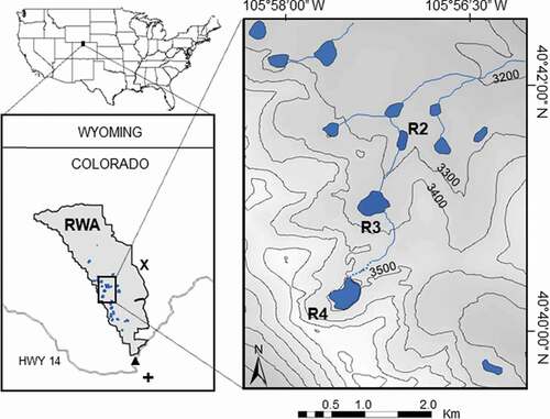
The focus of this study was lakes in the Rawah Wilderness Area (RWA) of north central Colorado (Figure 1). These glacial lakes range in elevation from 3,100 to 3,500 m.a.s.l. As is true of most high elevation lakes across the western United States, the RWA lakes are small (<20 ha), and many of them are paternoster lakes connected by a stream (Bahls 1992; Horne and Goldman 1994). The hydrology of the RWA is also similar to that of other montane areas of the Western United States, with inflows dominated by snowmelt dynamics (Poff and Ward 1990). Historically, the ice-free season for high elevation lakes in Colorado lasted from June until October (Roberts et al. 2017). Based on our sampling and modeling (Christianson, Johnson, and Hooten 2020), we estimate that about one third of the twenty-five named lakes in RWA are currently polymictic and the remainder are dimictic. Because changes to inflow magnitude and timing, as well as warmer air temperatures, could increase the chances for polymictic lakes to stratify, we chose one polymictic lake (Rawah #2) and one dimictic lake (Rawah #3) for detailed study and comparison (Figure 1). The lakes are less than 1 km apart, so they experience the same weather conditions, but the outflow from Rawah #3 flows into Rawah #2. Rawah #3 is situated at 3,316 m.a.s.l., has a maximum depth of 35 m, mean depth of 10 m, and a surface area of 8.5 ha. Rawah #3 has an inflow also; Rawah #2 is situated at 3,275 m.a.s.l. and has a maximum depth of 4 m, mean depth of 1.2 m, and surface area of 2.8 ha. Both lakes contain naturally reproducing brook trout and cutthroat trout that are stocked biennially to sustain those populations; no other fish species are present (Colorado Parks and Wildlife, Fort Collins, CO, USA).

Figure 1. Raw Wilderness Area (RWA) of northern Colorado, United States, with location of the lakes in blue (R2 = Rawah #2, R3 = Rawah #3, R4 = Rawah #4) and approximate elevation topography (m.a.s.l.). The locations of the weather station (X), SNOTEL site (triangle), and Michigan River stream gauge (cross) are also shown

Data collection and hydroclimate scenarios

We used a combination of measurements and sensor data we collected and data from nearby Natural Resources Conservation Service Snow Telemetry (SNOTEL) and United States Geological Service stream gauge sites to estimate ice-off dates and to assemble the lake and local hydroclimatic data for our simulations. We developed air warming scenarios based on Intergovernmental Panel on Climate Change (2013) forecasts. For each hydroclimate scenario, we modeled lake temperatures mechanistically from ice-off until 31 August when our fieldwork concluded and extrapolated autumn lake surface temperatures using an empirically derived polynomial from collected data. We then used these growing season temperatures to compute growing degree days and simulated energetic implications for fish using a bioenergetics model.

We deployed water temperature and weather dataloggers to gather the information required to calibrate a thermodynamic lake model (described below) for the study lakes. Onset HOBO Pendant UA-002-08 dataloggers were used to collect hourly surface, bottom, and inflow temperatures of both lakes from May through August 2016. We deployed an Onset U30 remote weather station on the eastern border of the wilderness area, about 10 km from the study lakes, to collect air temperature (°C), wind speed (m/s), relative humidity (%), precipitation (rain; mm), and solar radiation (W/m²; Christianson, Johnson, and Hooten 2020). Cloud cover was calculated as a ratio of sampled solar radiation to clear sky radiation (ASCE-EWRI Task Committee Report 2005), and cloud cover was then used to calculate longwave radiation. A comparison with long-term records going back to the 1980s showed that weather in 2016 reasonably represented nominal weather conditions for the study area (Christianson, Johnson, and Hooten 2020).

Because of the remoteness of RWA lakes, little is known about ice-off dates, but snowpack melt (hereafter snowmelt) is linked to ice-out in other high elevation lakes (Parker, Vinebrooke, and Schindler 2008; Sadro, Melak, Sickman, and Skeen 2018). We used the date that snowpack was exhausted (snow water equivalent [SWE] = 0; hereafter, “snowmelt date”) to approximate the initiation of lake surface warming (Figure 2). Ice-off date was assumed to occur when lake surface temperatures reached 4°C (Wetzel 2001; Roberts et al. 2017). We used snowpack/snowmelt data from the “Joe Wright” (551) SNOTEL site, which was located at an elevation of 3,571 m and <0.5 km from the RWA boundary (Figure 1; National Water and Climate Center n.d.). SNOTEL data from 1980 to 2016 also allowed us to characterize the variability in snowpack and snowmelt dates and configure simulation scenarios. SNOTEL records showed that the snowmelt date in 2016 (16 June) was close to the long-term average (17 June; SD = 11 days, n = 37 years), again suggesting that 2016 was a reasonable representation of nominal hydroclimatic conditions for the study area.

The lowest snowpack and earliest snowmelt date on record occurred in 2012 (Figure 3); data from that year were used to represent the early snowmelt scenario. Annual snowpack (maximum SWE) was positively correlated with snowmelt date (r = 0.80, N = 36, p < .01; Figure 3), suggesting that variation in snow deposition accounted for some of the annual variation in snowmelt dates. It was also shown that snowmelt date was associated with lake warming (Figure 2). In 2016, both lakes began warming shortly after snow depth reached zero, but it took over a week longer to reach ice-free conditions. Rawah #2 became ice free nine days after SWE reached zero, whereas Rawah #3 took 11 days to become ice free.

Figure 2. Daily snowpack depth (SWE) and lake surface temperatures and inflow temperature for Rawah #2 and Rawah #3 in 2016, as well as outflow temperature for Rawah #2. Date of ice-out in each lake is indicated. Polynomial functions fit to the inflows are shown as dotted lines

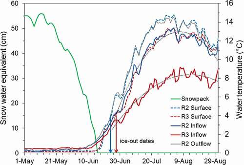
Figure 3. (a) Day of year when snowpack reached zero (snowmelt date; solid line) and yearly maximum snowpack depth (SWE; dashed line). (b) Frequency histogram of snowmelt dates. All snow data are from the Joe Wright SNOTEL station in north central Colorado, United States

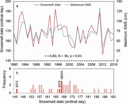
Figure 4. Streamflow from the Michigan River stream gauge for 2012 and 2016 (solid lines). Fitted exponential decay functions are shown for the duration of the open-water period each year (dotted lines)

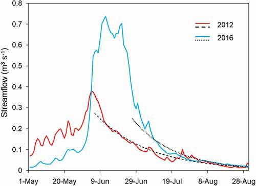
As in other federally designated wilderness areas, stream gauges do not exist in the RWA, so we used streamflow data from the stream gauge closest to the RWA (gauge number 06614800, “Michigan River”; Figure 1) and at a similar elevation (3,167 m.a.s.l.; RMRS 2019) to characterize the timing of the descending limb of the hydrograph of lake inflows under nominal (2016) and early snowmelt (2012) conditions (Figure 4). An exponential decay function (Martinec 1975) was fitted to the stream gauge data for these two years. This decay function was of the form

(1) $Q=R_0{e}^{-Kt}$(1)

where Q is daily inflow (m³ s⁻¹), R₀ is initial daily runoff, K is the coefficient of exhaustion, and t is day. Total inflow to each lake was estimated during model calibration (Christianson, Johnson, and Hooten 2020), and that discharge entered the lakes according to each year’s exponential decay function. We used temperatures of inflows to Rawah #2 and Rawah #3 recorded in 2016 to represent nominal inflow temperatures. Rawah #2 inflow temperatures were close to Rawah #3 surface temperatures (Figure 2), so Rawah #3 surface temperature was used as Rawah #2 inflow temperature. For Rawah #3 inflow temperature during early snowmelt, we fit a second-order polynomial to the nominal daily inflows (R² > 0.96; Figure 2) and shifted them to the earlier snowmelt date. Weather conditions (described above) in 2016 were used for nominal and early snowmelt scenarios.

We simulated effects of air temperature rise with two scenarios: (a) nominal temperatures +2°C and (b) nominal temperatures +5°C. These increases represent (a) the most probable and (b) the extreme predictions of air warming for this region, corresponding to representative concentration pathways of 4.5 and 8.5 (Intergovernmental Panel on Climate Change 2013). Nominal (2016) air temperatures were increased by these amounts for each warming scenario. We increased the temperature of inflows to Rawah #3 in warming scenarios using an adjustment of 0.44°C per 1°C increase in air temperature (Mohensi, Erickson, and Stefan 1999; Rieman and Isaak 2010). Predicted surface temperatures in Rawah #3 were used for Rawah #2 inflow temperatures.

Thermodynamic modeling

We used the General Lake Model v3.1.1 (GLM; Hipsey et al. 2012) in R v3.3.2 (R Core Team 2016) to simulate surface temperatures in the study lakes under nominal conditions (2016) and under altered hydroclimate scenarios. The GLM is a one-dimensional, process-based thermodynamic model that simulates water temperature profiles while accounting for dynamic processes like mixing, inflows, outflows, and the surface energy balance. The model has been used worldwide for a variety of lake types and conditions (Hipsey et al. 2017; Winslow et al. 2017; Bruce et al. 2018; Christianson, Johnson, and Hooten 2020). As have others studying lakes of similar sizes, clarities, and elevations (Bruce et al. 2018; Christianson, Johnson, and Hooten 2020), we used parameter values recommended by Hipsey et al. (2017; see table 2 in Bruce et al. 2018). Model inputs included a time series of meteorological data and lake-specific data (depth, area, latitude, longitude, light attenuation coefficient, and inflow temperatures and discharge).

First, we calibrated GLM to match 2016 observed surface temperatures in each lake by varying inflow (see Read et al. 2014; Bueche and Vetter 2015; Magee and Wu 2016; Bruce et al. 2018; Fenocchi et al. 2018; Christianson, Johnson, and Hooten 2020) to minimize the root mean square error (RMSE) of measured and simulated epilimnion temperatures:

(2) $\mathrm{R}\mathrm{M}\mathrm{S}\mathrm{E}=\sqrt{\frac{\sum _{i=1}^N{\left(Pre{d}_i-Ob{s}_i\right)}^2}{N}}$(2)

where N is the number of observations, Pred_i is the predicted daily average surface temperature, and Obs_i is the observed daily average surface temperature. Inflows were validated by comparing estimated flows to stream flows from a nearby gauge at similar elevation and in situ inflow estimates (see Christianson, Johnson, and Hooten 2020). Simulations for each lake began at ice-off; in 2016 Rawah #2 became ice free on 25 June and Rawah #3 became ice free on 27 June (Figure 2). Simulations continued until 31 August when our fieldwork concluded. We then used the calibrated model to simulate effects of alternative snowmelt date and air temperature scenarios. Ice-off dates for earlier snowmelt scenarios (4 June in Rawah #2 and 6 June for Rawah #3) were estimated using the same delay between snowmelt date and ice-free date as observed during nominal conditions. We then compared lake surface temperature regimes under nominal (2016) and altered hydroclimatic conditions.

In total we simulated lake temperatures in six hydroclimate scenarios: nominal conditions, nominal +2°C air warming, nominal +5°C air warming, early snowmelt with nominal air temperatures, early snowmelt with +2°C air warming, and early snowmelt with +5°C air warming. Each scenario was applied to each lake, and surface temperatures were tracked. Because Rawah #2 is very shallow, surface temperature was estimated from averaging surface and bottom temperatures assuming that the lake would remain polymictic (Christianson, Johnson, and Hooten 2020). The overall thermal effects of each scenario were quantified by calculating growing degree days for the simulation period:

(3) $DD=\sum _{i=1}^{N}max\left(T_{dail{y}_i}-T_{bas{e}_i},0\right)$(3)

where DD is cumulative degree days, N is the number of days in the simulation, T_daily are daily average simulated temperatures, and T_base is baseline temperature. We used T_base = 4°C because this temperature represents the minimum temperature for growth of salmonids (Piper et al. 1982; Wedemeyer 2001; Roberts et al. 2017; Christianson et al. 2019). The number of days in simulations differed because starting dates varied with snowmelt date. Because the growing season extends beyond the date of intensive data collection and our GLM simulations (31 August), we extrapolated lake temperatures and DD until lake temperature reached 4°C in the fall using a second-order polynomial function fitted (R² = 0.96) to the simulated lake temperature for each scenario. We included these additional DD to demonstrate how thermal conditions may vary beyond 31 August, but we do not include these additional days to assess bioenergetic effects due to the lack of empirical data.

Bioenergetics effects

We assessed the effects of earlier snowmelt and air temperature scenarios on physiological responses of the fishes using the temperature output from each hydroclimate scenario in a bioenergetics model. Bioenergetics models are based on the second law of thermodynamics, which implies that the energy consumed by a fish (its ration) is balanced by the energy expended for metabolism, wastes, and growth (Brett and Groves 1979; Deslauriers et al. 2017):

(4) $C=M+W+S+G$(4)

where C is consumption, M is metabolism, W is waste products, S is somatic growth, and G is gonadal growth. Model parameters are species specific, and physiological relationships are functions of temperature and body size. Units for each term are typically in joules per day, but mass equivalents can be computed from the energy density of the fish and its food (e.g., Johnson, Pate, and Hansen 2017). These models have been used to address a wide variety of ecological questions, but commonly they have been used to evaluate how diet or environmental conditions affect fish growth or to quantify effects of a predator on its prey (Hewett and Johnson 1987; Hanson et al. 1997; Deslauriers et al. 2017). Under a given set of environmental conditions, the amount of growth (somatic or gonadal) a fish can attain, its “scope for growth,” is a function of its consumption and metabolic losses:

(5) $SFG=C-\left(M+W\right)$(5)

where SFG is scope for growth, C is consumption, M is metabolism, and W is waste products. When SFG = 0, no energy is available to allocate to growth or reproduction, but the fish must consume enough food to compensate for losses to metabolism and wastes (the maintenance ration). Thus, setting SFG = 0 is a sensible way to quantify the effects of environmental change on minimum energy requirements for a fish, when future food availability and consumption rate are unknown. Any growth or reproduction would require additional energy intake above this baseline.

We used Bioenergetics 4.0 v1.1.1 (Beauchamp, LaRiviere, and Thomas 1995; Hartman and Cox 2008; Deslauriers et al. 2017) in R to model the effects of hydroclimate scenarios on the energetics of two cold-adapted salmonid species present in the study lakes and common in high elevation lakes of the region: cutthroat trout and brook trout. These species have been the top two species stocked in Colorado mountain lakes for decades (Nelson 1988). Bioenergetics simulations lasted from ice-out until 31 August, and we tracked daily respiration rate (J/g/d) and the total amount of food required for maintenance over the simulation period (SFG = 0). We simulated one size class (171 g wet weight) of fish of each species. Trout in mountain lakes of the RWA and across the SRM are typically small, reaching reproductive maturity by this size (Nelson 1988; Downs 1995; Young 1995; Kennedy, Peterson, and Fausch 2003; Belk, McGee, and Shiozawa 2009), and this size is representative of catchable trout (~250 mm total length) vulnerable to recreational anglers of the region (Nelson 1987). Diets of fish in small mountain lakes are dominated by invertebrates, including amphipods, dipterans, and zooplankton (Cavalli et al. 1997; Carlisle and Hawkins 1998; Schindler, Knapp, and Leavitt 2001). Energy densities of these taxa range from 2,050 to 4,090 J/g wet mass (James et al. 2012), so we used a value of 3,000 J/g for generic prey energy density in our simulations. Energy density of the fish was set to 4,000 J/g (Johnson, Pate, and Hansen 2017) based on energy densities measured in similar-sized rainbow trout (Oncorhynchus mykiss) and brown trout (Salmo trutta) in another high elevation lake in Colorado (Johnson, Pate, and Hansen 2017).

Results

Thermodynamic modeling

After model calibration, simulated water temperatures were in good agreement with observed temperatures for both lakes. The RMSE for Rawah #3 was 1.22°C for surface temperatures and 0.14°C for bottom temperatures, and the RMSE for Rawah #2 was 1.12°C for surface and 1.27°C for bottom temperatures. Simulated inflow volumes and temperature coefficients in the calibrated GLM simulations are provided in Table 1.

Table 1. Values of coefficients used to simulate lake inflow temperature and volume. $Temp=a{t}^2+bt+c$$R_0{e}^{-Kt}$

				Lake
Inflow parameter	Snowmelt scenario	Model coefficient	Air warming scenario	Rawah #2	Rawah #3
Volume	Nominal	R0		2.7	2.2
		K		−0.072	−0.072
	Early	R0		2.7	2.2
		K		−0.057	−0.057
Temperature	Nominal	a	Nominal		−0.0022
			+2°C		−0.0022
			+5°C		−0.0022
		b	Nominal		0.3541
			+2°C		0.3541
			+5°C		0.3541
		c	Nominal		−6.1194
			+2°C		−4.1194
			+5°C		−1.1194
	Early	a	Nominal		−0.0014
			+2°C		−0.0014
			+5°C		−0.0014
		b	Nominal		0.21
			+2°C		0.21
			+5°C		0.21
		c	Nominal		0.5
			+2°C		1.38
			+5°C		2.7

Note. Values correspond to a second-order polynomial for temperature: $Temp=a{t}^2+bt+c$, where t is the ordinal day starting on 26 May (i.e., when snow depth reached zero in 2012), and an exponential decay for volume: Flow = $R_0{e}^{-Kt}$, where t is the same as temperature, R₀ is initial flow, and K is the extinction coefficient. Rawah #3 surface temperatures were used for Rawah #2 inflow temperatures.

Air temperature increases and early snowmelt both affected lake surface temperatures (Figure 5). Air warming had a larger effect on average and maximum surface temperatures than early snowmelt. Early snowmelt increased surface temperatures by approximately 0.8°C, on average, but air warming increased surface temperatures by 1.3°C at +2°C and 2.4°C at a + 5°C on average. Rawah #2 was warmer than Rawah #3 by 0.7°C on average. Maximum surface temperatures differed between the two lakes. Maximum surface temperatures in Rawah #2, which was polymictic, were 14.8°C, 16.2°C, and 17.6°C under nominal, +2°C, and +5°C air temperatures, respectively. Maximum surface temperatures in Rawah #3 (dimictic) were 15.4°C, 16.6°C, and 18.1°C for the three air temperature scenarios.

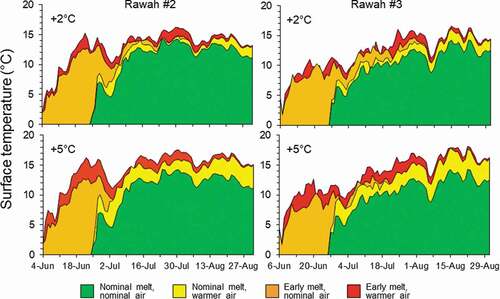
Early snowmelt allowed for warming to begin sooner in both lakes, accumulating more heat early in the summer, whereas nominal snowmelt buffered against early lake surface warming (Figure 5). However, by the end of summer, lake surface temperatures were only about 1°C higher in the early vs. nominal snowmelt scenarios. Differences in surface temperatures between snowmelt scenarios were greater throughout the summer and slightly higher at the end of summer in Rawah #3. Spring warming and fall cooling were more rapid in Rawah #2 under both snowmelt scenarios.

Figure 5. Predicted effects of air temperature and snowmelt scenarios on lake surface temperatures of Rawah #2 (left) and Rawah #3 (right)

Early snowmelt also resulted in more heat accumulation over the open water season than did increased air temperature (Figure 6). Averaged across lakes, early snowmelt increased growing degree days by 42 percent, whereas a 2°C increase in air temperatures only increased growing degree days by 12 percent, and a 5°C increase in air temperatures only increased growing degree days by 26 percent. Early snowmelt and air warming together increased average growing degree days by 54 percent at +2°C and 70 percent at +5°C. Growing degree days accumulated by the end of August were always higher in Rawah #2, due to earlier ice out and onset of warming. However, Rawah #2 also cooled more quickly in the fall, so by the end of the season total growing degree days was higher in Rawah #3 under all hydroclimate scenarios. Earlier snowmelt and warming both produced higher proportional increases in growing degree days at Rawah #3 than at Rawah #2, suggesting that stratification may have made Rawah #3 surface temperatures more sensitive to climate change effects than surface temperatures in the polymictic lake.

Figure 6. Predicted growing degree days in the study lakes under nominal conditions vs. increased air temperature and earlier snowmelt scenarios. Percentages show relative change from nominal conditions for the simulation period. Growing degree days extrapolated after 31 August until water temperature reached 4°C in autumn are also shown

Bioenergetics effects

Under nominal conditions, brook trout had lower median daily respiration rates than cutthroat trout in both lakes, and brook trout had a wider range of daily respiration rates in all scenarios (Figure 7). In general, air temperature rise had a larger effect on daily metabolic costs than did snowmelt recession. Daily respiration rates increased slightly for both species in the early snowmelt scenario and much more in the air warming scenarios. Averaged across species and lakes, respiration rate increased by 15 and 38 percent in the +2°C and +5°C air temperature scenarios, respectively, compared with only 9 percent in the early snowmelt scenario. Average respiration rates increased by 25 percent at +2°C and 46 percent at +5°C in combination with early snowmelt. In most scenarios, the median daily respiration rate was higher in Rawah #2 but only slightly greater than in Rawah #3, which had a larger range in daily respiration rates.

Figure 7. Mean specific respiration rates of cutthroat trout and brook trout during ice-off to August 31 in Rawah #2 (A) and Rawah #3 (B) under six hydroclimate scenarios

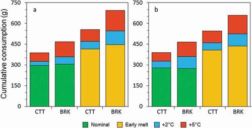
Unlike daily respiration rates, earlier snowmelt had a larger effect on cumulative metabolic costs (measured as the seasonal maintenance ration) than air temperature rise, and the effect was greater for brook trout (Figure 8). Both species of trout would need to consume more food to compensate for the effects of earlier snowmelt than for the effects of warmer air temperatures. Across lakes, the average maintenance ration with +2°C and +5°C warming respectively increased by 13.8 and 21.9 percent for cutthroat trout and 23.8 percent and 37.4 percent for brook trout. The average increase in food required with earlier snowmelt was 43.4 percent for cutthroat trout and 52.3 percent for brook trout. Combined effects of +5°C warming and earlier snowmelt could approximately double the minimum food requirements for these two species (92 percent for cutthroat trout and 133 percent for brook trout).

Figure 8. Predicted cumulative consumptive demand of cutthroat trout (CTT) and brook trout (BRK) in (a) Rawah #2 and (b) Rawah #3 during ice-off to 31 August across hydroclimate scenarios: nominal air temperatures and nominal snowmelt (green), nominal air temperatures and early snowmelt (orange), and the additional effect of 2°C (blue) and 5°C (red) warmer air temperatures on each snowmelt scenario

Discussion

Many studies of the effects of climate change on lakes have focused on the effects of air temperature rise (e.g., Kettle et al. 2004; Missaghi, Hondzo, and Herb 2017; Woolway et al. 2017; Prats and Danis 2019). Our findings suggest that future predictions may underestimate the impact of climate change on lake temperatures, growing season length, and fish energetic demands if reduced snowpack and earlier snowmelt and ice-off dates coincide with rising air temperatures. An increase in growing season length alone could be equivalent to the effects of moderate increases to air temperature. In our simulations, air temperature rise was constrained to a maximum of 5°C, based on a representative concentration pathway of 8.5, though a 2°C increase is considered more likely to occur in the future. On the other hand, growing season length increased by twenty-one days in our simulations, based on historical observations, and could be more in the future, so changes to growing season length have the potential to affect seasonal heat accumulation more than air temperature rise. The largest effect would occur when a longer growing season coincides with increased air temperature.

We treated air temperature rise as an additive effect on growing season attributes and independent of snowpack, and we did not consider effects of interannual variability. Reality is more variable and complex. Air temperature rise is not independent of other hydroclimatic features; for example, air temperature rise itself may hasten snowmelt through sensible heat exchange but also via greater occurrence of rain on snow events (Berg and Hall 2017). Even during high snowpack years, rain on snow and increased air temperatures may drive early melt. Further, when coupled with increased air temperature and rain events, low snowpack years could result in earlier melt dates than observed so far. Although snowpack has decreased for some regions (Fyfe et al. 2017), generally, future snowpack is uncertain (Kharin et al. 2013). However, due to the possibility that air temperature increases will drive earlier average snowmelt regardless of snowpack conditions, early snowmelt and longer growing seasons are likely to become more frequent if air temperatures continue to climb.

Another study in the SRM estimated a recession in mountain lake ice-off date of 2.1 days/decade (Preston et al. 2016). If this trend is applicable to our lakes, it would mean that by 2100, the new average ice-off date would occur within about four days of 2012, the most extreme year on record. Shorter periods of snow cover and warmer growing seasons could also have indirect effects on mountain lakes such as more forest fires and decreased stream flows (Hoffman, Fountain, and Achuff 2007; Clow 2010; Aponte, de Groot, and Wotton 2016). These watershed impacts can affect lake clarity and inflows (Barnett, Adam, and Lettenmaier 2005; Bixby et al. 2015) and amplify direct effects of air temperature rise on lake temperatures (Christianson, Johnson, and Hooten 2020). For example, air warming combined with reduced clarity and inflow could be double the effects of air warming alone (Christianson, Johnson, and Hooten 2020). Thus, in combination with earlier snowmelt and air warming, secondary climate change effects could cause unprecedented increases in lake temperature. In addition, because many mountain lakes are connected by streams to form paternoster systems, rising lake temperatures will have implications for downstream stream and lake temperatures as well.

As we showed, streamflow from melting snowpack buffers lakes from warming, but this effect is diluted if inflows are received from an upstream lake. We found that inflows from our upstream lake (Rawah #3) to the downstream lake (Rawah #2) were more than 4°C warmer in late summer than the inflows to Rawah #3. Thus, the presence of lakes can significantly alter downstream stream temperatures, and these lakes can amplify the effect of warmer air temperatures on streams, especially in years with low snowpack and earlier snowmelt. Therefore, studies on the effect of climate change on mountain stream temperatures and the effectiveness of the “cold-water climate shield” for salmonid refugia (Isaak et al. 2015) should consider the presence of lakes and the indirect effect of earlier snowmelt on stream temperature change.

Climate change could also affect the availability of thermal refugia for fish within the lakes themselves. The direct and indirect effects of warmer and longer growing seasons can intensify lake stratification (Christianson, Johnson, and Hooten 2020), increasing the opportunity for hypoxia to develop in the hypolimnion (Jankowski et al. 2006). Many of the lakes in our study area already exhibit hypoxia during late August (Christianson, Johnson, and Hooten 2020). Thus, longer growing seasons in the future may restrict lacustrine fish to warmer surface waters, with implications for habitat choice and their energy budgets.

Overall, we found that early snowmelt alone had a greater effect on growing degree days and total energy demand of fishes than even the most extreme commonly accepted predictions of air temperature rise, primarily due to its effects on growing season length. Early snowmelt was predicted to have relatively modest effects on daily energy demand (respiration rates) because summer lake temperatures rose by only about 1°C over temperatures exhibited during an average snowmelt year. However, early snowmelt allowed lake warming to begin three weeks earlier and result in the accumulation of 47 percent more growing degree days for trout in our study lakes. The longer growing season and higher number of growing degree days meant that trout would need to consume almost 50 percent more food to meet basic metabolic demands and considerably more food to gain surplus energy to devote to growth. Increases to growing degree days due to earlier snowmelt would provide additional opportunity for fish to grow if sufficient food resources are present. It should be noted that our estimates of trout food requirements show relative differences across species and hydroclimate scenarios but do not include consumption after 31 August. Total food requirements for the entire growing season could be up to 50 percent higher, based on our extrapolated growing degree days.

Air temperature rise had larger effects on daily energy demand than early snowmelt. Despite this, the cumulative effect over the growing season was generally less than the effects of early snowmelt. The effect of a 2°C increase in daily air temperatures increased average daily energy demand by an amount similar to that caused by earlier snowmelt, but if daily air temperatures rose by 5°C, then average daily respiration rates exceeded those under early snowmelt. Cumulative energy demand of brook trout was slightly more sensitive to air temperature rise than that of cutthroat trout, and a 5°C increase in air temperatures could have a slightly greater effect for that species than earlier snowmelt. Maximum lake temperatures were close to the optimum for growth of both species (~14°C) and well below maximum temperature for growth (~20°C; Schofield et al. 1993; Bear, McMahon, and Zale 2007) in all scenarios. This implies that growth of trout in these lakes in the future will not be temperature limited and that growth could actually increase given adequate food resources.

Our predictions of the effects of climate change on the growing season and fish energy demands have important implications for growth and survival of these sport fish as well as for their competitive interactions. If food is sufficient, the longer growing season resulting from early snowmelt could allow trout to attain larger sizes. Indeed, other work showed that another coldwater salmonid, brown trout, grew 50 percent more in an alpine lake during low snowpack/early snowmelt years (Borgstrøm 2001). Historic growth rates of cutthroat trout and brook trout in the RWA lakes are moderate, with fish achieving 314 and 289 mm by age five, respectively (Nelson 1987), which is slightly below the generally accepted fisheries-defined “quality” size for these species (Neumann, Guy, and Willis 2012). Thus, faster growth with warmer water could be achievable and would be appreciated by anglers.

Effects of climate change on food production in these mountain lakes have not been investigated, so it is difficult to predict how future fish growth will actually be affected. Most mountain lakes in the region are oligotrophic (Bahls 1992), but warmer temperatures and longer growing seasons could increase primary and secondary production, potentially increasing food availability for fish. Oleksy (2019) demonstrated that recent warming combined with nitrogen deposition in the SRM increased the production of benthic algae. Food for fish could increase if amphipods, dipterans, and other benthic invertebrates common in mountain lake fish diets respond to increases in primary production. However, mountain lakes are complex systems that do not respond equally across the landscape. Some studies suggest that production has increased in mountain lakes (Hundey et al. 2014; Jiminez et al. 2017; Moser et al. 2019) via atmospheric deposition of nitrogen, phosphorus, and calcium. However, catchment characteristics and nutrient limitation vary among lakes, and it is unknown how nutrient deposition will be affected by fossil fuel combustion and agricultural nutrient transport in the future. If in-lake food production lags behind expected climate-driven increases in trout consumptive demand, then competitive interactions that are well documented for these two species (Kennedy, Peterson, and Fausch 2003) could intensify, and growth and survival may decrease. More research is needed to forecast how thermal effects of a changing climate will affect mountain lake thermal conditions and productivity and therefore how fish populations may respond.

The historic range of snowmelt dates for this region was greater than six weeks, and the SD was just under two weeks. The extreme scenario we simulated occurred once in 37 years. Thus, natural variability in snowmelt date is already high, but very early snowmelt has been rare. Natural year-to-year variation in snowmelt has been a feature of these systems, but a directional change toward earlier snowmelt could have an additive effect on fish energetics because both species can live for more than five years in these lakes (Nelson 1987). Successive years of early snowmelt and high consumptive demand could impact survival if food is scarce but could result in substantial increases in size at age if food availability increases with growing degree days.

Conclusions

We showed that low snowpack resulting in early snowmelt can increase mountain lake temperatures, heat accumulation, growing season length, and fish consumptive demand in our study system. We found that these effects could be more than twice as strong as expected climate-driven changes in air temperature. Mountain lakes in other regions may respond differently depending on local climatic conditions and the relative importance of snowpack and air temperature regime on ice cover duration and growing season length. In snowmelt-driven systems like ours, changes to these lake and biotic features would be even more important if snowmelt recession and air temperature rise coincide in the future. Uncertainty in how mountain lake productivity will be affected by climate change makes it difficult to know whether climate change will be beneficial or detrimental to fish populations. Given potential increases in food requirements for fish but poor ability to forecast changes in food availability, managers will need to monitor fish growth rates to determine whether changes to stocking rates or other actions are necessary to maximize sport fish production as climate and lake productivity change. The higher sensitivity of lake thermal conditions and fish energy requirements to snowpack dynamics also highlights the need to include changes to snowfall and snowmelt in forecasting the effects of climate change on mountain lakes and their biota.

Acknowledgments

We thank Ben Galloway, Casey Barby, Brendon Sucher, Austin Coward, and William Pate for help in collecting field data. Comments by Scott Denning, Mevin Hooten, and Chris Myrick improved the article.

Additional information

Funding

This project was supported by NSF Grant No. DGE-0966346 “I-WATER: Integrated Water, Atmosphere, Ecosystems Education and Research Program” and a private gift to Colorado State University, account number 6-464540.

References

- Adrian, R., C. M. O’Reilly, H. Zagarese, S. B. Baines, D. O. Hessen, W. Keller, D. M. Livingstone, R. Sommaruga, D. Straile, E. Van Donk, et al. 2009. Lakes as sentinels of climate change. Limnology and Oceanography 54:2283–97. doi:https://doi.org/10.4319/lo.2009.54.6_part_2.2283.
- Aponte, C., W. J. de Groot, and B. M. Wotton. 2016. Forest fires and climate change: Causes, consequences and management options. International Journal of Wildland Fire 25. doi:https://doi.org/10.1071/WFv25n8_FO.
- ASCE-EWRI. 2005. The ASCE standardized reference evapotranspiration equation. Technical Committee Report to the Environmental and Water Resources Institute of the American Society of Civil Engineers from the Task Committee on Standardization of Reference Evapotranspiration. Reston, VA: ASCE-EWRI.
- Bahls, P. 1992. The status of fish populations and management of high mountain lakes in the Western United States. Northwest Science 66:183–93.
- Barnett, T. P., J. C. Adam, and D. P. Lettenmaier. 2005. Potential impacts of a warming climate on water availability in snow-dominated regions. Nature 438:303–09. doi:https://doi.org/10.1038/nature04141.
- Bear, E. A., T. E. McMahon, and A. V. Zale. 2007. Comparative thermal requirements of westslope cutthroat trout and rainbow trout: Implications for species interactions and development of thermal protection standards. Transactions of the American Fisheries Society 136:1113–21. doi:https://doi.org/10.1577/T06-072.1.
- Beauchamp, D. A., M. G. LaRiviere, and G. L. Thomas. 1995. Evaluation of competition and predation as limits to the production of juvenile sockeye salmon in Lake Ozette. North American Journal of Fish Management 15:121–35. doi:https://doi.org/10.1577/1548-8675(1995)015<0193:EOCAPA>2.3.CO;2.
- Belk, M. C., M. N. McGee, and D. K. Shiozawa. 2009. Effects of elevation and genetic introgression on growth ofColorado River cutthroat trout. Western North American Naturalist 69:56–62. doi:https://doi.org/10.3398/064.069.0116.
- Benjamin, J. R., and C. V. Baxter. 2012. Is a trout a trout? A rangewide comparison shows nonnative brook trout exhibit greater density, biomass, and production than native inland cutthroat trout. Biological Invasions 14:1865–79. doi:https://doi.org/10.1007/s10530-012-0198-9.
- Berg, N., and A. Hall. 2017. Anthropogenic warming impacts on California snowpack during drought. Geophysical Research Letters 44:2511–18. doi:https://doi.org/10.1002/2016GL072104.
- Bixby, R. J., S. D. Cooper, R. E. Gresswell, L. E. Brown, C. N. Dahm, and K. A. Dwire. 2015. Fire effects on aquatic ecosystems: An assessment of the current state of the science. Freshwater Science 34:1340–50. doi:https://doi.org/10.1086/684073.
- Borgstrøm, R. 2001. Relationship between spring snow depth and growth of Brown Trout, Salmo trutta, in an alpine lake: Predicting consequences of climate change. Arctic, Antarctic, and Alpine Research 33:476–80. doi:https://doi.org/10.1080/15230430.2001.12003457.
- Brett, J. R., and T. D. D. Groves. 1979. Physiological energetics. In Fish physiology: Bioenergetics and growth, ed. W. S. Hoar, D. J. Randall, and J. R. Brett, 279–352. New York: Academic Press.
- Brubaker, K. L. and A. Rango. 1996. Response of snowmelt hydrology to climate change. Water, Air and Soil Pollution 90:335–43.
- Bruce, L. C., M. A. Frassl, G. B. Arhonditsis, G. Gal, D. P. Hamilton, P. C. Hanson, A. L. Hetherington, J. M. Melack, J. S. Read, K. Rinke, et al. 2018. A multi-lake comparative analysis of the General Lake Model (GLM) stress-testing across a global observatory network. Environmental Modelling & Software 102:274291. doi:https://doi.org/10.1016/j.envsoft.2017.11.016.
- Bueche, T., and M. Vetter. 2015. Future alterations of thermal characteristics in a medium-sized lake simulated by coupling a regional climate model with a lake model. Climate Dynamics 44:371–84. doi:https://doi.org/10.1007/s00382-014-2259-5.
- Carlisle, D. J., and C. P. Hawkins. 1998. Relationships between invertebrate assemblage structure, two trout species, and habitat structure in Utah mountain lakes. Journal of the North American Benthological Society 17:266–300. doi:https://doi.org/10.2307/1468332.
- Cavalli, L., R. Chappaz, P. Bouchard, and G. Brun. 1997. Food availability and growth of the brook trout, Salvelinus fontinalis (Mitchill), in a French Alpine lake. Fisheries Management and Ecology 4:167–77. doi:https://doi.org/10.1046/j.1365-2400.1997.00116.x.
- Christianson, K. R., B. M. Johnson, and M. B. Hooten. 2020. Compound effects of water clarity, inflow, wind and climate warming on mountain lake thermal regimes. Aquatic Sciences 82. doi:https://doi.org/10/1007/s00027-019-0676-6.
- Christianson, K. R., B. M. Johnson, M. B. Hooten, and J. J. Roberts. 2019. Estimating lake climate responses from sparse data: An application to high elevation lakes. Limnology and Oceanography 64:1371–85. doi:https://doi.org/10.1002/lno.11121.
- Clow, D. W. 2010. Changes in the timing of snowmelt and streamflow in Colorado: A response to recent warming. Journal of Climate 23:2293–306. doi:https://doi.org/10.1175/2009JCLI2951.1.
- Deslauriers, D., S. R. Chipps, J. E. Breck, J. A. Rice, and C. P. Madenjian. 2017. Fish bioenergetics 4.0: An R-based modeling application. Fisheries 42:586–96. doi:https://doi.org/10.1080/03632415.2017.1377558.
- Dibike, Y., T. Prowse, T. Saloranta, and R. Ahmed. 2011. Response of Northern Hemisphere lake-ice cover and lake-water thermal structure patterns to a changing climate. Hydrological Processes 25:2942–53.
- Downs, C. C. 1995. Age determination, growth, fecundity, age at sexual maturity, and longevity for isolated, headwater populations ofwestslope cutthroat trout. Thesis, Montana State University, Bozeman.
- Dunham, J. B., S. B. Adams, R. E. Schroeter, D. C. Novinger. 2002. Alien invasions in aquatic ecosystems: Toward an understanding of brook trout invasions and potential impacts on inland cutthroat trout in western North America. Reviews in Fish Biology and Fisheries 12:373–91. doi:https://doi.org/10.1023/A:1025338203702.
- Eby, L. A., W. Roach, L. Crowder, and J. Stanford. 2006. Effects of stocking-up freshwater food webs. Trends in Ecology & Evolution 21:576584. doi:https://doi.org/10.1016/j.tree.2006.06.016.
- Fenocchi, A., M. Rogora, S. Sibilla, M. Ciampittiello, and C. Dresti. 2018. Forecasting the evolution in the mixing regime of a deep subalpine lake under climate change scenarios through numerical modelling (Lake Maggire, Northern Italy/Southern Switzerland). Climate Dynamics 51:3521–36. doi:https://doi.org/10.1007/s00382-018-4094-6.
- Ficke, A. D., C. A. Myrick, and L. J. Hansen. 2007. Potential impacts of global climate change on freshwater fisheries. Reviews in Fish Biology and Fisheries 17:581–613. doi:https://doi.org/10.1007/s11160-007-9059-5.
- Fyfe, J. C., C. Derksen, L. Mudryk, G. M. Flato, B. D. Santer, N. C. Swart, N. P. Molotch, X. Zhang, H. Wan, V. K. Arora, et al. 2017. Large near-term projected snowpack loss over the western United States. Nature Communications 8. doi:https://doi.org/10.1038/ncomms14996.
- Hanson, P. C., T. B. Johnson, D. E. Schindler, and J. F. Kitchell. 1997. Fish bioenergetics 3.0 technical report WISCU-T-97-001, University of Wisconsin Sea Grant Institute, Madison.
- Hartman, K. J., and M. K. Cox. 2008. Refinement and testing of a brook trout bioenergetics model. Transactions of the American Fisheries Society 137:357–63. doi:https://doi.org/10.1577/T05-243.1.
- Hewett, S. W., and B. J. Johnson. 1987. A generalized bioenergetics model of fish growth for microcomputers. Sea Grant Tech. Rept. WIS-SG-87-245, University of Wisconsin, Wisconsin Sea Grant College Program, Madison.
- Hipsey, M. R., L. C. Bruce, C. Boon, B. Busch, C. C. Carey, D. P. Hamilton, et al. 2017. A general lake model (GLM 2.4) for linking with high-frequency sensor data from the Global Lake Ecological Observatory Network (GLEON). Geoscientific Model Development Discussion. doi:https://doi.org/10.5194/gmd-2017-257.
- Hipsey, M. R., L. C. Bruce, C. Boon, J. Bruggeman, K. Bolding, and D. P. Hamilton. 2012. GLM-FABM v9.0a model overview and user documentation, 44. Perth, Australia: The University of Western Australia Technical Manual.
- Hoffman, M., A. Fountain, and J. Achuff. 2007. 20th-century variations in area of cirque glaciers and glacierets, Rocky Mountain National Park, Rocky Mountains, Colorado USA. Annals of Glaciology 46:349–54. doi:https://doi.org/10.3189/172756407782871233.
- Honsey, A. E., P. A. Venturelli, and N. P. Lester. 2018. Bioenergetic and limnological foundations for using degree-days derived from air temperatures to describe fish growth. Canadian Journal of Fisheries and Aquatic Sciences 76:657–69. doi:https://doi.org/10.1139/cjfas-2018-0051.
- Horne, A. J., and C. R. Goldman. 1994. Limnology. New York: McGraw-Hill.
- Hundey, E. J., K. A. Moser, F. J. Longstaffe, N. Michelutti, and R. Hladyniuk. 2014. Recent changes in production in oligotrophic Uinta Mountain lakes, Utah, identified using paleolimnology. Limnology and Oceanography 59:1987–2001. doi:https://doi.org/10.4319/lo.2014.59.6.1987.
- Intergovernmental Panel on Climate Change. 2013. Climate change 2013: The physical science basis. In Contribution of working group I to the fifth assessment report of the intergovernmental panel on climate change, eds. T. F. Stocker, D. Qin, G.-K. Plattner, M. Tignor, S. K. Allen, J. Boschung, A. Nauels, Y. Xia, V. Bex, and P. M. Midgley, 1535. Cambridge, UK: Cambridge University Press.
- Isaak, D. J., M. K. Young, D. E. Nagel, D. L. Horan, and M. C. Groce. 2015. The cold-water climate shield: Delineating refugia for preserving salmonid fishes through the 21st century. Global Change Biology 21:2540–53. doi:https://doi.org/10.1111/gcb.12879.
- James, D. A., I. J. Csargo, A. Von Eschen, M. D. Thul, J. M. Baker, C.-A. Hayer, J. Howell, J. Krause, A. Letvin, S. R. Chipps, et al. 2012. A generalized model for estimating the energy density of invertebrates. Freshwater Science 31:69–77. doi:https://doi.org/10.1899/11-057.1.
- Jankowski, T., D. M. Livingstone, H. Buhrer, R. Forster, and P. Niederhauser. 2006. Consequences of the 2003 European heat wave for lake temperature profiles, thermal stability, and hypolimnetic oxygen depletion: Implications for a warmer world. Limnology and Oceanography 51:815–19. doi:https://doi.org/10.4319/lo.2006.51.2.0815.
- Jiminez, L., K. M. Ruhland, A. Jeziorski, J. P. Smol, and C. Perez-Martinez. 2017. Climate change and Saharan dust drive recent cladoceran and primary production changes in remote alpine lakes of Sierra Nevada, Spain. Global Change Biology. doi:https://doi.org/10.1111/gcb.13878.
- Johnson, B. M., W. M. Pate, and A. G. Hansen. 2017. Energy density and dry matter content in fish: New observations and an evaluation of some empirical models. Transactions of the American Fisheries Society 146:1262–78. doi:https://doi.org/10.1080/00028487.2017.1360392.
- Kennedy, B. M., D. P. Peterson, and K. D. Fausch. 2003. Different life histories of brook trout populations invading mid-elevation and high-elevation cutthroat trout streams in Colorado. Western North American Naturalist 63:215–23.
- Kettle, H., R. Thompson, N. J. Anderson, and D. M. Livingstone. 2004. Empirical modeling of summer lake surface temperatures in southwestGreenland. Limnology and Oceanography 49:271–82. doi:https://doi.org/10.4319/lo.2004.49.1.0271.
- Kharin, V. V., F. W. Zwiers, X. Zhang, and M. Wehner. 2013. Changes in temperature and precipitation extremes in the CMIP5 ensemble. Climatic Change 119:345–57. doi:https://doi.org/10.1007/s10584-0130705-8.
- Kirillin, G. 2010. Modeling the impact of global warming on water temperature and seasonal mixing regimes in small temperate lakes. Boreal Environment Research 15:279–93.
- Knapp, R. A. 1996. Nonnative trout in natural lakes of the Sierra Nevada: An analysis of their distribution and impacts on native aquatic biota. In Sierra Nevada ecosystem project: Final report to Congress, vol. III, 363–407. Davis: Centers for Water and Wildland Resources, University of California. ceres.ca.gov/snep/pubs.
- Lisi, P. J., D. E. Schindler, T. J. Cline, M. D. Scheuerell, and P. B. Walsh. 2015. Watershed geomorphology and snowmelt control stream thermal sensitivity to air temperature. Geophysical Research Letters 42:3380–88. doi:https://doi.org/10.1002/2015GL064083.
- Luoto, T. P., and L. Nevalainen. 2013. Long-term water temperature reconstructions from mountain lakes with different catchment and morphometric features. Scientific Reports 3:1–5. doi:https://doi.org/10.1038/srep02488.
- Magee, M. R., and C. H. Wu. 2016. Response of water temperatures and stratification to changing climate in three lakes with different morphometry. Hydrology and Earth System Sciences Discussion. doi:https://doi.org/10.5194/hess-2016-262.
- Magnuson, J. J., D. M. Robertson, B. J. Benson, R. H. Wynne, D. M. Livingstone, T. Arai, R. A. Assel, et al. 2000. Historical trends in lake and river ice cover in the Northern Hemisphere. Science 289:1743–46. doi:https://doi.org/10.1126/science.289.5485.1743.
- Marnell, L. F., R. J. Behnke, and F. W. Allendorf. 1987. Genetic identification of cutthroat trout, Salmo clarki, in Glacier National Park, Montana. Canadian Journal of Fisheries and Aquatic Sciences 44:1830–39. doi:https://doi.org/10.1139/f87-227.
- Martinec, J. 1975. Snowmelt – runoff model for stream flow forecasts. Nordic Hydrology 6:145154. doi:https://doi.org/10.2166/nh.1975.0010.
- McGrath, C. C., and W. M. Lewis. 2007. Competition and predation as mechanisms for displacement of greenback cutthroat trout by brook trout. Transactions of the American Fisheries Society 136:1381–92. doi:https://doi.org/10.1577/T07-017.1.
- Meyer, K. A., and D. J. Schill. 2007. Multistate high mountain lake summit. IDFG Report 07-55, Idaho Department of Fish and Game, Boise.
- Michelutti, N., A. Labaj, C. Grooms, and J. P. Smol. 2016. Equatorial mountain lakes show extended periods of thermal stratification with recent climate change. Journal of Limnology 75. doi:https://doi.org/10.4081/jlimnol.2016.1444.
- Missaghi, S., M. Hondzo, and W. Herb. 2017. Prediction of lake water temperature, dissolved oxygen, and fish habitat under changing climate. Climatic Change 141:747–57. doi:https://doi.org/10.1007/s10584017-1916-1.
- Mohensi, O., T. R. Erickson, and H. G. Stefan. 1999. Sensitivity of stream temperatures in the United States to air temperature projected under a global warming scenario. Water Resources Research 35:3723–33. doi:https://doi.org/10.1029/1999WR900193.
- Moser, K. A., J. S. Baron, J. Brahney, I. A. Oleksy, J. E. Saros, E. J. Hundey, S. A. Sadro, J. Kopáček, R. Sommaruga, M. J. Kainz, et al. 2019. Mountain lakes: Eyes on global environmental change. Global and Planetary Change 178:77–95. doi:https://doi.org/10/1016/j.gloplacha.2019.04.001.
- Mote, P. W., A. F. Hamlet, M. P. Clark, and D. Lettenmaier. 2005. Declining mountain snowpack in western North America. Bulletin of the American Meteorological Society 86:39–49. doi:https://doi.org/10.1175/BAMS-86-1-39.
- Musselman, K. N., M. P. Clark, C. Liu, K. Ikeda, and R. Rasmussen. 2017. Slower snowmelt in a warmer world. Nature Climate Change 7:214–19. doi:https://doi.org/10.1038/nclimate3225.
- National Water and Climate Center. n.d. Natural Resources Conservation Service. US Department of Agriculture. http://www.wcc.nrcs.usda.gov/snow/
- Nelson, W. C. 1987. Survival and growth of fingerling trout planted in high lakes of Colorado. Technical Publication 36, Colorado Division of Wildlife, Fort Collins.
- Nelson, W. C. 1988. High lake research and management in Colorado. Special Report 64, Colorado Division of Wildlife, Fort Collins.
- Neumann, R., C. Guy, and D. Willis. 2012. Length, weight, and associated indices. In Fisheries techniques, ed. A. V. Zale, D. L. Parrish, and T. M. Sutton, 637676. 3rd ed. Bethesda, MD: American Fisheries Society.
- O’Reilly, C. M., S. Sharma, D. K. Gray, S. E. Hampton, J. S. Read, R. J. Rowley, et al. 2015. Rapid and highly variable warming of lake surface waters around the globe. Geophysical Research Letters 42:10,773–10,781. doi:https://doi.org/10.1002/2015GL066235.
- Oleksy, I. A. 2019. Algal blooms in the alpine: Investigating the coupled effects of warming and nutrient deposition on mountain lakes. Fort Collins, CO: Colorado State University Libraries.
- Parker, B. R., R. D. Vinebrooke, and D. W. Schindler. 2008. Recent climate extremes alter alpine lake ecosystems. Proceedings of the National Academy of Sciences of the United States of America 105:12927–31. doi:https://doi.org/10.1073/pnas.0806481105.
- Pepin, N., R. S. Bradley, H. F. Diaz, M. Baraer, E. B. Caceres, N. Forsythe, et al. 2015. Elevation-dependent warming in mountain regions of the world. Nature Climate Change 5:424–30. doi:https://doi.org/10.1038/nclimate2563.
- Piper, R. G., I. B. McElwain, L. E. Orme, J. P. McCraren, L. G. Fowler, and J. R. Leonard. 1982. Fish hatchery management. Washington, D.C: U.S. Fish and Wildlife Service.
- Poff, N. L., and J. V. Ward. 1990. Physical habitat template of lotic systems: Recovery in the context of historical pattern of spatiotemporal heterogeneity. Environmental Management 14:629–45. doi:https://doi.org/10.1007/BF02394714.
- Prats, J., and P. Danis. 2019. An epilimnion and hypolimnion temperature model based on air temperature and lake characteristics. Knowledge and Management of Aquatic Ecosystems 8. doi:https://doi.org/10/1051/kmae/2019001.
- Preston, D. L., N. Caine, D. M. McKnight, M. W. Williams, K. Hell, M. P. Miller, S. J. Hart, and P. T. J. Johnson. 2016. Climate regulates alpine lake ice cover phenology and aquatic ecosystem structure: Climate and alpine lakes. Geophysical Research Letters 43:5353–60. doi:https://doi.org/10.1002/2016GL069036.
- R Core Team. 2016. R: A language and environment for statistical computing. Vienna, Austria: R Foundation for Statistical Computing. http://www.R-project.org/.
- Railsback, S. F., and K. A. Rose. 1999. Bioenergetics modeling of stream trout growth: Temperature and food consumption effects. Transactions of the American Fisheries Society 128:241–56. doi:https://doi.org/10.1577/1548-8659(1999)128<0241:BMOSTG>2.0.CO;2.
- Read, J. S., L. A. Winslow, G. J. A. Hansen, J. Van Den Hoek, P. C. Hanson, L. C. Bruce, and C. D. Markfort. 2014. Simulating 2368 temperate lakes reveals weak coherence in stratification phenology. Ecological Modelling 291:142–50. doi:https://doi.org/10.1016/j.ecolmodel.2014.07.029.
- Rieman, B. E., and D. J. Isaak. 2010. Climate change, aquatic ecosystems, and fishes in the Rocky Mountain West: Implications and alternatives for management. General Technical Report. RMRS-GTR-250, U.S. Department of Agriculture, Forest Service, Rocky Mountain Research Station, Fort Collins, CO, 46.
- RMRS (Rocky Mountain Research Station). 2019. Western U.S. stream flow metrics. United States Department of Agriculture, Forest Service, Boise, ID. Accessed February 2019. https://www.fs.fed.us/rm/boise/AWAE/projects/modeled_stream_flow_metrics.shtml.
- Roberts, J. J., K. D. Fausch, D. P. Peterson, and M. B. Hooten. 2013. Fragmentation and thermal risks from climate change interact to affect persistence of native trout in the Colorado river basin. Global Change Biology 19:1383–98. PMID: 23505098. doi:https://doi.org/10.1111/gcb.12136.
- Roberts, J. J., K. D. Fausch, T. S. Schmidt, and D. M. Walters. 2017. Thermal regimes of Rocky Mountain lakes warm with climate change. PloS One 12:e0179498. doi:https://doi.org/10.1371/journal.pone.0179498.
- Sadro, S., J. M. Melack, J. O. Sickman, and K. Skeen. 2018a. Climate warming response of mountain lakes affected by variations in snow. Limnology and Oceanography Letters. doi:https://doi.org/10.1002/lol2.10099.
- Sadro, S., J. O. Sickman, J. M. Melack, and K. Skeen. 2018b. Effects of climate variability on snowmelt and implications for organic matter in a high-elevation lake. Water Resources Research 54:4563–78. doi:https://doi.org/10.1029/2017WR022163.
- Schindler, D. E., R. A. Knapp, and P. R. Leavitt. 2001. Alteration of nutrient cycles and algal production resulting Griffiths 94 from fish introductions into mountain lakes. Ecosystems 4:308–21. doi:https://doi.org/10.1007/s10021-001-0013-4.
- Schmid, M., S. Hunziker, and A. Wüest. 2014. Lake surface temperatures in a changing climate: A global sensitivity analysis. Climatic Change 124:301–15. doi:https://doi.org/10.1007/s10584-014-1087-2.
- Schofield, C. L., D. Josephson, C. Keleher, and S. P. Gloss. 1993. Thermal stratification of dilute lakes—an evaluation of regulatory processes and biological effects before and after base addition effects: Effects on brook trout habitat and growth. U.S. Fish and Wildlife Service Biological Report NEC93/9. Washington, DC: U.S. Fish and Wildlife Service.
- Sharma, S., K. Blagrave, J. J. Magnuson, C. M. O’Reilly, S. Oliver, R. D. Batt, M. R. Magee, D. Straile, G. A. Weyhenmeyer, L. Winslow, et al. 2019. Widespread loss of lake ice around the Northern Hemisphere in a warming world. Nature Climate Change Letters 9:227–31. doi:https://doi.org/10.1038/s41558-018-0393-5.
- Thompson, R., D. Price, N. Cameron, V. Jones, C. Bigler, P. Rosén, R. I. Hall, J. Catalan, J. García, J. Weckstrom, et al. 2005. Quantitative calibration of remote mountain-lake sediments as climatic recorders of air temperature and ice-cover duration. Arctic, Antarctic, and Alpine Research. 37 (4):626–35. doi:https://doi.org/10.1657/1523-0430(2005)037[0626:QCORMS]2.0.CO;2.
- Tranvik, L. J., J. A. Downing, J. B. Cotner, S. A. Loiselle, R. G. Striegl, T. J. Ballatore, P. Dillon, K. Finlay, K. Fortino, L. B. Knoll, et al. 2009. Lakes and reservoirs as regulators of carbon cycling and climate. Limnology and Oceanography 54:2298–314. doi:https://doi.org/10.4081/jlimnol.2005.139.
- Wedemeyer, G. A., ed. 2001. Fish hatchery management. 2nd ed., 733. Bethesda, MD: American Fisheries Society.
- Wenger, S. J., D. J. Isaak, C. H. Luce, H. M. Neville, K. D. Fausch, J. B. Dunham, D. C. Dauwalter, M. K. Young, M. M. Elsner, B. E. Rieman, et al. 2011. Flow regime, temperature, and biotic interactions drive differential declines of trout species under climate change. Proceedings of the National Academy of Sciences of the United States of America 108:14175–80. doi:https://doi.org/10.1073/pnas.1103097108.
- Wetzel, R. G. 2001. Limnology: Lake and river ecosystems. San Diego, CA: Academic Press.
- Winslow, L. A., G. J. A. Hansen, J. S. Read, K. C. Rose, and M. Notaro. 2017. Large-scale modeled contemporary and future water temperature estimates for 10,774 midwestern U.S. Lakes. Scientific Data 4. doi:https://doi.org/10.1038/sdata.2017.53.
- Woolway, R. I., and C. J. Merchant. 2019. Worldwide alteration of lake mixing regimes in response to climate change. Nature Geoscience 12:271–76. doi:https://doi.org/10.1038/s41561-019-0322-x.
- Woolway, R. I., M. T. Dokulil, W. Marszelewski, M. Schmid, D. Bouffard, and C. J. Merchant. 2017. Warming of Central European lakes and their response to the 1980s climate regime shift. Climatic Change 142:505–20. doi:https://doi.org/10.1007/s10584-017-1966-4.
- Yarnell, S. M., J. H. Viers, and J. F. Mount. 2010. Ecology and management of the spring snowmelt recession. BioScience 60:114–27. doi:https://doi.org/10.1525/bio.2010.60.2.6.
- Young, M. K. 1995. Chapter 2. Colorado River Cutthroat Trout. In Conservation assessment for inland cutthroat trout. General Technical Report RM-256, ed. M. K. Young tech., 16–23. Fort Collins, CO: U.S. Dept. of Agriculture, Forest Service, Rocky Mountain Forest and Rang Experiment Station.
- Yvon-Durocher, G., J. I. Jones, M. Trimmer, G. Woodward, and J. M. Montoya. 2010. Warming alters the metabolic balance of ecosystems. Philosophical Transactions of the Royal Society B 365:2117–26. doi:https://doi.org/10.1098/rstb.2010.0038.