Timing of Little Ice Age maxima and subsequent glacier retreat in northern Troms and western Finnmark, northern Norway

ABSTRACT

Glaciers are important indicators of climate change, and recent observations worldwide document increasing rates of mountain glacier recession. Here we present approximately 200 years of change in mountain glacier extent in northern Troms and western Finnmark, northern Norway. This was achieved through (1) mapping and lichenometric dating of major moraine systems within a subset of the main study area (the Rotsund Valley) and (2) mapping recent (post-1980s) changes in ice extent from remotely sensed data. Lichenometric dating reveals that the Little Ice Age (LIA) maximum occurred approximately 1814 (±41 years), which is before the early twentieth-century LIA maximum proposed on the nearby Lyngen Peninsula but younger than LIA maximum limits in southern and central Norway (mid-eighteenth century). Between LIA maximum and 1989, a small sample of measured glaciers (n = 15) shrank a total of 3.9 km² (39 percent), and those that shrank by more than 50 percent are fronted by proglacial lakes. Between 1989 and 2018, the total area of glaciers within the study area (n = 219 in 1989) shrank by approximately 35 km². Very small glaciers (<0.5 km²) show the highest relative rates of shrinkage, and 90 percent of mapped glaciers within the study area were less than 0.5 km² in 2018.

KEYWORDS:

• Glacier change
• remote sensing
• lichenometry
• ‘Little Ice Age’
• northern Norway

Introduction

The most recent period of Holocene glacier expansion is termed the Little Ice Age (LIA; Grove 2001, 2004). Initiating around 1300, the LIA triggered a global, yet asynchronous, advance of glaciers (Solomina et al. 2016). In many regions, the turn of the twentieth century marked the end of the LIA, with glaciers having entered a period of sustained retreat, interrupted by only minor, localized glacier advances (Overpeck et al. 1997; Grove 2004; Winkler, Elvehøy, and Nesje 2009; data from NVE 2016). The observed glacial retreat since the LIA has been linked to the anthropogenically forced warming during the twentieth and early twenty-first centuries (IPCC 2019). With these trends set to continue, climate warming is likely to be greatly amplified in Arctic regions (Serreze and Barry 2011). This Arctic amplification is expected to increase mean annual air temperatures within the Arctic Circle by between 4.2°C and 8.3°C (Najafi, Zwiers, and Gillett 2013; IPCC 2019). There is therefore increasing concern about the response of Arctic ice and snow to anthropogenically forced climate change.

In Norway, 2,534 glaciers cover an area of approximately 2,692 km² (Andreassen, Winsvold, et al. 2012), with an estimated volume of 271 ± 28 km³ (Andreassen et al. 2015), which if melted completely would contribute an estimated 0.34 mm of sea level rise (Nesje et al. 2008). There is also substantial importance of Norwegian glaciers in relation to energy supply, environmental hazards, and tourism (Andreassen, Winsvold, et al. 2012; Furunes and Mykletun 2012; Jackson and Ragulina 2014; Xu et al. 2015). Furthermore, Norwegian glaciers are particularly sensitive to climate fluctuations due to their maritime location, with their mass balance heavily influenced by large-scale atmospheric circulation patterns (e.g., Arctic Oscillation and North Atlantic Oscillation; Nesje, Lie, and Dahl 2000; Thompson and Wallace 2000; Rasmussen 2007; Nesje and Matthews 2011; Bonan, Christian, and Christianson 2019). Norway is therefore a prime location to study the response of glaciers to climate change, but there remain several glacierized regions in Norway that lack detailed investigation (Stokes et al. 2018). In particular, the mapping and dating of LIA glacier extent and subsequent retreat has only been done for a small number of glaciers and glacier regions in Norway (e.g., Ballantyne 1990; Bickerton and Matthews 1993; Winkler 2003; Matthews 2005; Nussbaumer, Nesje, and Zumbühl 2011; Weber et al. 2019), and most of the small glacierized sites within northern Troms lack investigation as to their LIA limits. As such, it is unclear when glaciers reached their LIA maximum in this region and how rates of glacial change have varied after this maximum.

In this article, we (a) compile detailed geomorphological maps and conduct fieldwork to identify and date LIA moraines (using lichenometry); (b) compare glacier area changes from historical maps and previous glacier inventories, dating from 1907 to 1966; and (c) undertake new analysis of satellite imagery (30–15 m spatial resolution) and aerial orthophotographs (<1 m spatial resolution) to map glacier area change over the period 1989 to 2018.

Study area

The area of investigation is in northern Norway and covers approximately 9,600 km². It is located predominantly in northern Troms county but crosses into Finnmark county on the Bergsfjord Peninsula (Figure 1). The study region is characterized by a range of different glacier sizes; in the northeast on the Bergsfjord Peninsula (region C; Figure 1), ice caps and outlet glaciers dominate, whereas in the mountain belts throughout the central and western regions (regions A and B; Figure 1), valley and cirque glaciers dominate. Due to the close proximity of large fjord systems and the North Atlantic Ocean, the majority of glaciers in the region are maritime, with relatively high precipitation during the winter and a smaller difference between winter and summer temperature averages than those experienced at similar latitudes inland (Andreassen, Kjøllmoen, et al. 2012). For example, between 1995 and 2018 the January and July mean temperature and total precipitation in the maritime setting of Tromsø (69°39′ N, 18°56′ E) were −3.1°C/2,344 mm and 12.3°C/1,788 mm, respectively. In contrast, the continental climate at Finnmarksvidda (69°22′ N, 24°26′ E; station # 97350) has January and July mean temperatures and total precipitation of −13.6°C/455 mm and 13.4°C/1,728 mm, respectively (data from eKlima 2019). The Inventory of Norwegian Glaciers (henceforth referred to as Andreassen, Winsvold, et al. 2012) defines our study area as “Region 3–Troms North” and “Region 2–Øksfjord”. The glacier inventory covering these two regions is based on Landsat imagery from 2001 and 2006. In total, Andreassen, Winsvold, et al. (2012) record 141 glaciers across both regions and provide details on their area, elevation (minimum and maximum), slope, and aspect. The glaciers range in size from 0.01 to 11.95 km². Only approximately 10 percent of the glaciers in this region are greater than 1 km² in area, but they account for approximately 67 percent of the total glacier area, whereas approximately 82 percent of glaciers are less than 0.5 km² but account for only approximately 23 percent of the total glacierized area (all values from Andreassen, Winsvold, et al. 2012).

Figure 1. Study area location in Troms and Finnmark county, northern Norway. The white rectangle represents the area under investigation, defined as “Region 3–Troms North,” and the gray rectangle shows “Region 2–Øksfjord” (Andreassen, Winsvold, et al. 2012). Turquoise rectangles indicate the three glacial regions, defined as A, B, and C (the Bergfjord Peninsular). The yellow rectangle shows the location of the field site within the Rotsund Valley. The location of the Rotsundelv churchyard (RC) and Storslett churchyard (SC) used for lichenometric dating controls are highlighted along with the location of the weather station at Sørkjosen Airport (SA). Note: The base image is a 2018 pan-sharpened Landsat 8 scene displayed as a false color composite; red–green–blue as 5-4-3

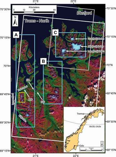
Nearly all prior glaciological research within the broad study area (Figure 1) has focused on the ice caps and outlet glaciers of the Bergsfjord Peninsula (region C; Figure 1). Data from the Bergsfjord Peninsula as a whole found highly nonlinear responses of local plateau-based icefields to climate changes during the Younger Dryas and throughout the Holocene (Gellatly et al. 1988; Evans et al. 2002; Rea and Evans 2007). Of particular interest is the Langfjordjøkelen ice cap, where annual mass balance records are available from 1989. The Langfjordjøkelen mass balance records reveal mass deficits throughout the period of observation and higher glacier retreat rates compared to elsewhere in Norway (Andreassen, Kjøllmoen, et al. 2012; Giesen et al. 2014; Wittmeier et al. 2015; Kjøllmoen 2019; Andreassen et al. 2020).

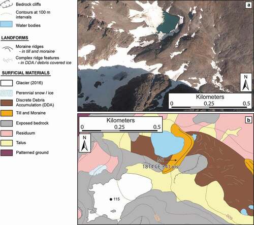
To address the lack of data on LIA limits in northern Troms, we identified a suitable field site in the Rotsund Valley in the Nordreisa municipality (Figure 1). The field site hosts very well-developed moraines fronting several small glaciers within part of a minor mountain range (colloquially referred to as the Kåfjord Alps), with mountain peaks ranging from 1,077 to 1,320 m a.s.l. The bedrock is composed of Vaddas Nappe and Kåfjord Nappe, broadly comprising metamorphic units of amphibolite, quartzite, gneiss, and schist (Lindahl, Stevens, and Zwaan 2005; Augland et al. 2014; Geological Survey of Norway 2015). To the west is a major fjord system, Lyngenfjord, and there are also subsidiary fjords north (Rotsundet) and south (Kåfjorden; Figure 1). The present-day tree line extends to approximately 400 m a.s.l. and, above this, alpine tundra is the dominant vegetation. The nearest weather station is at Sørkjosen Airport, approximately 11 km from the field site (SA; Figure 1), and has been operational since 2008 (# 91740: www.eKlima.no). Average monthly temperature typically varies from −10°C to 15°C; precipitation primarily falls as snow between October and May and rainfall can occur throughout the year (Vikhamar-Schuler, Hanssen-Bauer, and Førland 2010).

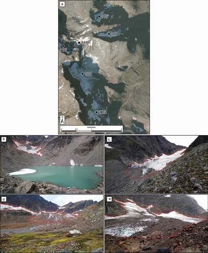
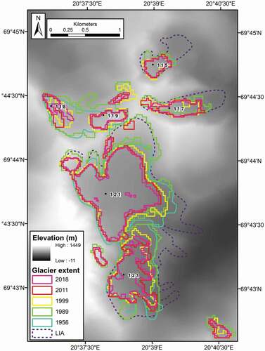
The four glaciers under investigation in the Rotsund Valley (glacier IDs 115, 117, 121, and 123; Figure 2) are located below 1,100 m a.s.l. As of 2018 the smallest glacier is glacier 115, with an area of 0.07 km² terminating approximately 760 m a.s.l. Glacier 115 is also the only glacier in the field site with a proglacial lake (0.3 km² and <200 m from the terminus; Figure 2b). The largest glacier is glacier 121 with an area of 0.8 km², terminating at approximately 650 m a.s.l. (Figure 2d). The other two glaciers 117 and 123 have areas of 0.11 and 0.3 km² and terminate approximately 730 and 600 m a.s.l., respectively (Figures 2c and Figure 2e). Within the forelands of glaciers 115, 117, 121, and 123 moraines occur as both individual features and as multiple ridges forming part of larger moraine systems. Throughout the area, distinct moraines are intermixed with areas of glacifluvial sediments and discrete debris accumulations (sensu Whalley 2009, 2012), exhibiting complex (hummocky) ridge features, and in the recently deglaciated terrain the moraines often border areas of till. The glacial forelands are sparsely vegetated, and the moraines surveyed are unobscured by trees or shrubs. The forelands of all four glaciers were surveyed in the field in August–September 2018, enabling the ground truthing of remotely sensed maps alongside lichenometric dating of moraines.

Figure 2. (A) 2016 Aerial orthophotographs (NORGEiBILDER 2019) of the Rotsund Valley field site. Photographs of the four glaciers visited in the field: (B) 115, (C) 117, (D) 121, and (E) 123. The dashed red line denotes the glacier extent in 2018

Data sets and methods

Geomorphological mapping

Geomorphological mapping of the Rotsund Valley field site (yellow rectangle in Figure 1) was conducted using georectified orthophotographs from https://www.norgeibilder.no at 0.25 m resolution, from various time steps (courtesy of the the Norwegian Mapping Authority). Using photographs from different time steps allowed for identification of features under different snow conditions and/or shading. Some late-lying snow was present in the imagery at time of capture (16 September 2016); however, this was removed in the maps based on the mapping done in the field and through cross-checking on imagery from differing time steps.

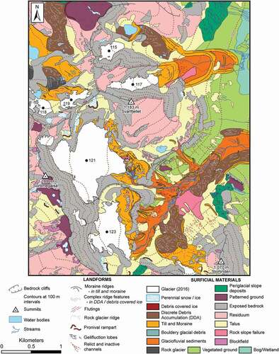
The geomorphological map was constructed using a three-stage process: Draft maps were digitized from analysis of orthophotographs, which were ground checked in the field, and a final stage of remotely sensed mapping then synthesized all three stages (Chandler et al. 2018). The resulting map (Figure 3) was used to reconstruct past glacier extent in the Rotsund Valley, in combination with the lichenometric dating of the moraines. In total, twenty-six different features were mapped and broadly classified as “landforms” (e.g., moraine ridges, flutings, pronival ramparts) or “surficial materials” (e.g., glacier, glaciofluvial sediments, talus) following methods employed for the mapping of Icelandic glaciated landsystems (e.g., Evans, Ewertowski, and Orton 2017a, 2017b, 2019).

The LIA moraines were initially identified based on their geomorphological form (large, sharp-crested, little evidence of slumping and/or reworking), together with a pronounced vegetation trimline. Though not vegetation free, the vegetation on these moraines is predominantly scrub vegetation with sporadic larger pioneer species, whereas moraines further down valley are fully vegetated with grasses, shrubs, and trees. Moraines dated by lichenometry are labeled from M1 (oldest/furthest from glacier front) to M8 (youngest/closest to glacier front).

Lichenometry

Lichen size data were collected from moraines within the forelands of glaciers 115, 117, 121, and 123 (see Figures 2 and 3). Lichenometric measurements were constrained to the yellow-green Rhizocarpon Ram. em. Th. Fr. subgen. Rhizocarpon lichen (Bickerton and Matthews 1993; Winkler 2003; Armstrong 2011). The diameter of the longest axis of each lichen thalli was measured using a flexible tape to the nearest millimeter (Innes 1986). Spherical and nonspherical lichens were measured to account for the decrease in the proportion of lichens that have remained circular with time, and any lichens coalesced (fused) over time were avoided (Innes 1985, 1986; Harrison et al. 2006). We identified coalescence in lichens by presence of a visible black streak of lichen prothallus dividing the specimen (Bradwell 2010). To mitigate potential biases of incorporating anomalous lichen in our data analysis, any single lichen more than 20 percent larger than the next largest lichen was removed from the data set, as is standard practice within lichenometry (Calkin and Ellis 1980; Loso and Doak 2006; Solomina, Ivanov, and Bradwell 2010; Loso, Doak, and Anderson 2014; Pendleton et al. 2017).

Figure 3. Geomorphological map of the field site within the Rotsund Valley (location shown in Figure 1) showing glaciers 115, 117, 118, 119, 121, and 123. Map based on field mapping and aerial orthophotographs (image date 16 September 2016) with 0.25 m spatial resolution

Our dating was conducted by indirect lichenometry, which utilizes the correlation of lichen sizes on surfaces of unknown age with those on surfaces of known age (Beschel 1950). Indirect lichenometry provides calculated surface ages that are obtained with the use of calibrated dating curves (Matthews 2005). Initial construction of dating curves relies on the presence of lichen growing on surfaces of known age, such as headstones, buildings, and independently dated natural surfaces such as boulders on moraines of known age (e.g., Jomelli et al. 2008; Wiles, Barclay, and Young 2010). Within the field site there are no surfaces that can be independently dated; therefore, headstones in nearby churchyards were used as controls. The churchyards are in the villages of Rotsundelv (Figure 1) and Storslett (Figure 1), approximately 6 and 14 km away from the field site, respectively. On each headstone, all lichen were measured from both horizontal and vertical faces. It was noted that some headstones recorded the burial of multiple persons at different times and, when reviewing the data, it was clear that these headstones carried anomalously smaller lichen relative to the oldest burial date. We therefore inferred that the headstone had been cleaned before the new inscription was added and, in these instances, the younger date was used as the control age.

At the field site, lichen size data were collected from siliceous rocks on moraines. Where possible, each moraine was searched for the largest lichen on the distal slope, crest, and proximal slope, thereby mitigating against the influence of microenvironmental variations (Erikstad and Sollid 1986; Karlën and Black 2002; Leigh 2016). On the large, steep-sided, latero-frontal moraines (sometimes in excess of 10 m high) only the crests were searched, due to issues associated with vertical age gradients on these large features (Humlum 1978). Once a data set of the largest lichens from the entirety of the moraine had been collected, the mean of the five largest lichen (5LL) was used for analysis (Innes 1984; Jomelli et al. 2007; Roof and Werner 2011). Recent work has also revealed that the 5LL method is not demonstrably inferior to other methods (notably size frequency methods) that require larger lichen size data sets (Evans et al. 2019) and in turn require considerably longer periods of time for data collection (which is not always feasible). Overall, implementing the 5LL method provides the greatest comparability to other studies using lichenometric dating throughout Norway and other Arctic regions (e.g., Karlén 1979; Evans, Butcher, and Kirthisingha 1994; Winkler et al. 2003; Jansen et al. 2016).

LIA glacier area and length reconstructions

Our LIA reconstructions were based on lichenometric dating and both remotely sensed and field-based moraine mapping. Initially, LIA glacier area reconstructions were made for the four glacier forelands surveyed in the field (glaciers 115, 117, 121, and 123). To enable further comparisons of LIA glacier extent, extrapolation of field observations and lichenometric dating was made for eleven other valley/cirque glaciers within the same mountain belt (region A; Figure 1). No dating of moraine limits was made for the additional glaciers; therefore, to maintain a reasonable level of comparability, only those glacier forelands with well-defined moraines of visual form similar to those examined in the field (e.g., position down valley from present day glacier, within a marked vegetation trimline) were mapped (Baumann, Winkler, and Andreassen 2009).

To map LIA glacier area, we extrapolated more recent glacier outlines from the 1950s to fit our mapped LIA moraine limits. Following established methods, the oldest glacier outlines (i.e., those digitized from topographical maps or from remote sensing) were extrapolated to the moraine limits in the lower parts of the glacier, following the extent of lateral moraines or vegetation trimlines (Baumann, Winkler, and Andreassen 2009; Stokes et al. 2018). The extrapolation of glacier polygons for LIA area also involved the reconnection of fragmented ice bodies. For glacier reconstructions where no prior outlines were present (n = 7 glaciers), we instead extrapolated from our 1989 remotely sensed outlines to meet the LIA moraine limits. The Andreassen, Winsvold, et al. (2012) ice divides were also used to ensure that individual tributaries were mapped as individual glacier units. Furthermore, for all glaciers where LIA glacier reconstructions were mapped, we also recorded whether a proglacial lake was now present within the boundary of the LIA moraine. Finally, to map glacier length we used published glacier centerlines (Winsvold, Andreassen, and Kienholz 2014) and either extrapolated or trimmed them to match our glacier outlines. For many of the smaller glaciers included in our study, no prior glacier centerlines were available; therefore, these were created by manual digitization perpendicular to contours generated from the Norwegian Mapping Authority N50 Digital Terrain Map (https://kartkatalog.geonorge.no/metadata/e25d0104-0858-4d06-bba8-d154514c11d2).

Remote sensing of twentieth- to twenty-first-century glacier extent

Firstly, glacier outlines from historic 1:100,000 and 1:50,000 topographic maps were provided by the Norwegian Water Resources and Energy Directorate (NVE 2016). The glacier outlines (e.g., Figure 4) were compiled by Winsvold, Andreassen, and Kienholz (2014) and dated to 1907, 1952, 1954, 1955, and 1966. Secondly, new glacier outlines were created for this study using Landsat 5 TM, 7 ETM+, and 8 OLI imagery (courtesy of the U.S. Geological Survey 2019) from 1989 to 2018 at roughly five-year time steps, enabling intradecadal analysis. However, due to challenges in obtaining suitable imagery in maritime northern Norway, it was not always possible to maintain equally spaced time steps (Andreassen et al. 2008; Leigh et al. 2019).

Glacier change mapping was performed using a well-established semi-automated technique, whereby a band ratio image was developed from the raw multispectral imagery (e.g., TM band 3/TM band 5 on Landsat 5) and subsequently converted to a binary image (Andreassen, Winsvold, et al. 2012). Adding an additional threshold (e.g., band 1) is sometimes used; however, in our preliminary mapping it was not shown to provide marked inprovements and was not used. Once the band ratio image was produced, we then selected a threshold value to isolate glaciers from non-glaciers, which was visually optimized for each scene by comparing the binary image with a false color composite (bands 5-4-3 as red–green–blue) of the multispectral imagery (Raup et al. 2007; Racoviteanu et al. 2009; Paul et al. 2013). A median filter (3 × 3 kernel) was then applied to help reduce noise from isolated pixels outside the glaciers and to close small voids within the glaciers (Andreassen, Winsvold, et al. 2012). Finally, once initial glacier outlines had been generated, manual correction of mapped units was undertaken to account for glaciers cast under shadow and/or debris cover, terminating in proglacial lakes, or surrounded by late-lying snow or where lakes/snow patches were erroneously classified as glaciers (Raup et al. 2007; Andreassen, Winsvold, et al. 2012). To ensure accuracy in mapping, especially around areas of shade, each image was viewed using multiple band combinations of red–green–blue as 5-4-3, 4-3-2, and 3-2-1. Additionally, all units mapped on the 1989 satellite imagery, including those that were not included within Andreassen, Winsvold, et al. (2012), were cross-checked on freely available aerial imagery from varying time steps to validate their identification as glaciers (NORGEiBILDER 2019). When cross-checking the imagery, we assessed the presence of visual indicators of glaciers (crevasses, flow features and deformed stratification, multiple debris bands in ice, ice, bergschrunds, moraines, and unbroken snow accumulation) to categorize each potential glacier unit as a possible, probable, or certain glacier, following the glacier identification scoring system of Leigh et al. (2019). All units that were considered to score two or more were retained and classified accordingly (11–20 = certain glacier; 6–10 = probable glacier; 2–5 = possible glacier; Leigh et al. 2019), and any units scoring less than two (e.g., snow/perennial snow) were removed.

Due to the relatively course (30–15 m) resolution of Landsat imagery and the associated errors of glacier mapping at this resolution, a minimum size threshold of 0.01 km² was implemented (Paul et al. 2010; Leigh et al. 2019). Therefore, all units less than 0.01 km² on the 1989 imagery were omitted from our maps due to difficulty in differentiating them from a perennial snowpatch. If an individual glacier fragmented over time and any individual unit shrank below 0.01 km² it was no longer mapped. We acknowledge that a glacier unit below our size threshold does not mean that the glacier has disappeared.

In addition to the satellite imagery, a series of historical oblique aerial photographs of the Rotsund Valley field site were used to provide context for glacier mapping. The oblique photographs aided in the identification of glacier extent, enabled confirmation of glacier confluence, and helped in differentiating snow from ice. The photographs were taken in 1952 by the airline company Wilderøe’s Flyveselskap and offer an oblique view southwest into the Rotsund Valley.

Errors and uncertainty in glacier mapping and reconstructions

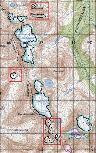
It is difficult to assess accuracy of the glaciers digitized from the 1:100,000 and 1:50,000 topographic maps, due to the undocumented methods used to map glaciers from the aerial photographs on which the topographic maps are based. Given that we use the same series of historical maps as Stokes et al. (2018), error estimates of the mapped glaciers are considered in line with their estimate of ±5 percent. It should be noted, however, that throughout the study region, approximately 20 percent of glaciers we have mapped were not included on the historic topographic maps (e.g., Figure 4).

Figure 4. Part of a Norwegian Mapping Authority 1:50,000 topographic map (map sheet: 1634 II) showing the digitized 1953 glacier outlines (turquoise) in the Rotsund Valley (yellow box in Figure 1). The 2001 Andreassen, Winsvold, et al. (2012) glacier outlines (black) are overlaid, with IDs shown. The red boxes highlight seven glaciers in this area that were not included on the 1953 topographic map. The two purple outlines are snow patches mapped in Andreassen, Winsvold, et al. (2012), one of which was initially mapped as a glacier on the 1953 map. Glaciers 115, 117, 121, and 123 are seen in Figure 3. For scale, grid squares are 1 × 1 km

Potential error associated with glacier mapping from satellite imagery relates not only to the extent to which a glacier’s boundaries can be identified and the accuracy of digitization (both of which are influenced with image resolution) but also to issues with georectification. Imagery was checked for georeferencing errors and any imagery that did not align was not used for mapping purposes. It should also be noted that identification of glacier boundaries is also influenced by external factors such as intensity of shading, snow cover, and supraglacial debris (Paul et al. 2013; Winsvold, Andreassen, and Kienholz 2014; Leigh et al. 2019). To assess the uncertainty from our semi-automated mapping, we used manually mapped glacier outlines from very high-resolution aerial orthophotographs (2016; 0.25 m resolution) as a benchmark from which we evaluated our glacier outlines from Landsat 8 and pan-sharpened Landsat 8 imagery (2016; 30 and 15 m resolution, respectively). Aerial imagery was used as a benchmark due to its very high resolution and accuracy of georectification compared to Landsat, meaning that we were able to most accurately define glacier boundaries even in areas of heavy shading. The mapping comparison was conducted for a subset of twenty-two glacier outlines, approximately 10 percent of the total number of glaciers mapped on the 1989 imagery (the first mapping time step). Mean percentage difference in glacier area between Landsat 8 imagery (30 m) and aerial orthophotographs (0.25 m) was ±9 percent and the mean percentage difference was ±6 percent between pan-sharpened Landsat 8 imagery (15 m) and aerial orthophotographs (0.25 m).

Estimates of error for the LIA areal extent based on our moraine mapping and dating are subject to uncertainties (in terms of both moraine ages and extrapolation of glacier area) that are difficult to quantify. The errors associated with LIA extrapolation are also a factor of moraine identification and preservation; where well-defined intact moraines are present it is easier to map glacier limits. In the case of our moraine mapping, we restricted the reconstructions to glacier forelands where well-defined end/latero-frontal moraines were identifiable on aerial imagery (e.g., Figure 5).

Climate data

There are no continuous, long-term meteorological records from within the study area. The nearest long-term record is from the city of Tromsø, located approximately 60 to 150 km to the west. Climate data were freely accessed via the Norwegian Meteorological Institute (eKlima 2019). In Tromsø, records are combined from station #90440 (located at 69°39′07.2″ N, 18°57′00.0″ E, 40 m a.s.l.) and station #90450 (located at 69°39′15.1″ N, 18°56′12.8″ E, 100 m a.s.l.) to gain a continuous record of temperature and precipitation from 1874 to 2018. Station #90440 was shut down in December 1926 and station #90450 was set up in July 1920, providing a period of overlap from which the older data can be homogenized. Following the approach of Andreassen, Kjøllmoen, et al. (2012) and Stokes et al. (2018), the mean of the difference between overlapping months was used to adjust the data prior to 1920. The homogenized temperature data were used to plot mean annual and seasonal temperature alongside total annual and seasonal precipitation and then also to calculate decadal means. Summer is defined as June–September and winter as October–May (Andreassen, Kjøllmoen, et al. 2012; Stokes et al. 2018).

Results

Dating moraines within the Rotsund Valley

Within the four surveyed forelands of the Rotsund Valley there were prominent glacial landforms that record a complex glacial history (Figure 3). Presumed LIA maximum moraines (termed M1 moraines throughout; see section Dating moraines within the Rotsund Valley.) were found between approximately 340 and 690 m a.s.l., and at the lower elevation they coincide with a pronounced vegetation trimline (Figure 5). Outside of the M1 moraines there are a series of large and well-vegetated moraines, sometimes extending down into the treeline and up to approximately 2 km from the present-day glacier termini.

Figure 5. Example of the LIA moraine examined in the field (foreland of glacier 121) that can be seen from (A) aerial orthophotograph (0.25 m resolution; NORGEiBILDER 2019) and (B) oblique photograph. The M1 moraine is sharp crested, with little evidence of slumping, predominantly unaffected by periglacial slope activity, and on the distal side of the moraine there is a distinct vegetation trimline. Note: The LIA moraines shown on the aerial imagery are not easily distinguishable on the 15 m Landsat imagery and not identifiable on the 30 m Landsat imagery

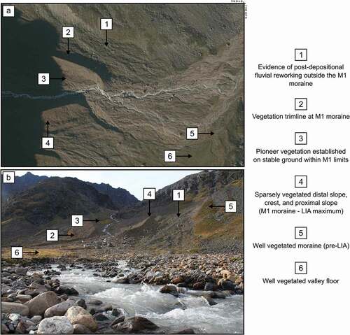
The forelands outside the M1 moraines lack tree cover but are often covered by an extensive mat of mountain crowberry (Empetrum nigrum), bilberry (genus Vaccinium), and various mosses (e.g., Racomitrium canescens and Polytrichum juniperinum), with dispersed yet well-established dwarf birch (Betula nana). Within the M1 moraines, where present, vegetation is predominantly grasses and small shrubs. When moving up valley (from the M1 moraines) vegetation becomes sparse, and once inside the M3 moraine, vegetation is almost nonexistent except for mosses and lichens.

Lichen size data and moraine ages since the LIA

The lichen size data collected in the field show a pronounced increase in lichen size (largest diameter) with distance from the glacier termini, confirming that lichen size is related to apparent substrate age. Table 1 shows the single largest lichen and 5LL for each moraine searched. To utilize lichenometry as a calculated age dating technique, we established a localized lichenometric dating curve (Figure 6). Our lichenometric dating curve was constructed from measurements of lichen growing on headstones within the Rotsundelv and Storslett churchyards (Figure 1). Once a plot of lichen size and surface age had been made, we used a logarithmic curve (y = 12.026ln(x) − 26.488, where x = years before 2018 and y = lichen size) plotted through the largest lichens following established methods (e.g., Innes 1983; Ballantyne 1990; Evans, Archer, and Wilson 1999). Due to the limited ages of the fixed points used in our site-specific dating, some extrapolation of the curve was unavoidable in order to calculate the ages of moraines that may be older than our oldest control data from the churchyards. Extrapolation of lichenometric dating curves is, however, common practice when sufficiently old control surfaces are rare, especially in remote regions (e.g., Ballantyne 1990; Evans, Archer, and Wilson 1999; Solomina, Ivanov, and Bradwell 2010). By using our site-specific dating curve (Figure 6), it was possible to assign calculated ages to the moraines within the Rotsund Valley. The resulting surface ages (years before 2018) range from 204 ± 41 years to 9 ± 2 years (Table 2), and the detailed moraine chronology for the studied glaciers in the Rotsund Valley is shown in Figures 7-10.

Table 1. Lichen size data (single largest lichen and mean of the 5LL) from the moraines within the four glacial forelands of the field site. Glacier IDs are provided as assigned within the Inventory of Norwegian Glaciers (Andreassen, Winsvold, et al. 2012)

Glacier ID	Moraine elevation (m a.s.l.)	Assigned moraine ID	Single largest lichen (mm)	5LL (mm)
115	660–690	M1	38	37.4
117	570–600	M1	35	33.2
	560–580	M2	32	26.5
	560–570	M3	24	23
121	340–440	M1	41	37
	360–380	M2	27	27
	595	M3	24	23.4
	545	M6	9	8.2
	555	M7	6	5.2
	570	M8	0	0
123	440–450	M1(1)	42	35.6
	425–500	M1(2)	35	33
	455–510	M2	30	23.6
	550–570	M4	14	13.2
	570	M5	13	11.2
	545–600	M6	8	7.4
	550	M8	0	0

Table 2. Results of the lichenometric dating providing calculated ages for the moraines under investigation

Glacier ID	Moraine	5LL (mm)	Calculated age (years before 2018)	Calculated age ±20% (years before 2018)	Date	Date ±20%
115	M1	37.4	204	245–163	1814	1773–1855
117	M1	33.2	143	172–114	1875	1846–1904
	M2	26.5	82	98–66	1936	1920–1952
	M3	23	61	73–48	1957	1945–1970
121	M1	37	196	235–157	1822	1783–1861
	M2	27	85.8	103–69	1932	1915–1949
	M3	23.4	63	76–50	1955	1942–1968
	M6	8.2	18	22–14	2000	1996–2004
	M7	5.2	14	17–11	2004	2001–2007
	M8	0	9	11–7	2009	2007–2011
123	M1(1)	35.6	175	175–140	1843	1808–1878
	M1(2)	33	140.5	169–112	1877	1849–1906
	M2	23.6	64	79–51	1954	1939–1967
	M4	13.2	27	32–22	1991	1986–1996
	M5	11.2	23	28–18	1995	1990–2000
	M6	7.4	17	20–14	2001	1998–2004
	M8	0	9	11–7	2009	2007–2011

Figure 6. Lichenometric dating curve constructed from lichen growth on dated headstones within the Rotsundelv and Storslett churchyards. The black line represents a logarithmic curve fitted to the largest lichens, and the dotted gray lines represent standardized ±20 percent lichenometric error margins. The curve has been extrapolated to represent lichen growth over the past 210 years

Figure 7. Geomorphological mapping of glacier 115 foreland; (A) aerial orthophotographs (NORGEiBILDER 2019; image date 19 September 2011) with 0.25 m spatial resolution showing the glacier foreland, (B) Geomorphological map of area shown in (A) showing the foreland of glacier 115 (Figure 2b) with annotations showing the moraine surveyed for lichenometry and the resulting calculated ages. Note:  Map based on field mapping and aerial orthophotographs from 2016 however, due to shading on the 2016 imagery on which the geomorphological map (B) is based, aerial imagery from 2011 (A) is shown

The M1 moraines exhibit a range of 5LL values from 33.2 to 37.4 mm (Table 1), with the oldest and youngest M1 moraine ages calculated at 204 and 196 years old (1814 [±41 years] and 1877 [±34 years]; Table 2, Figures 7–10). The M2 moraines have 5LL values between 23.6 to 27.0 mm and the associated ages vary between 82 and 64 years old (1936 [±16 years] and 1954 [±15 years]; Table 2, Figures 7–10). The younger moraines labeled M3 to M8 (where present) have a mixed range of calculated ages and, as a result, document a varying pattern of glacial advance and retreat between each glacier. The youngest moraines investigated are M8 moraines; these moraines are only present on the relatively flat forelands of glaciers 121 and 123, less than 300 m from the present-day glacier terminus (Figures 9 and 10). The M8 moraines carry no visible lichen specimens and, as a result, are given formation dates of approximately 2009, based on the lichen lag times established from the Rotsundelv and Storslett churchyards. The M8 moraine age is further supported by aerial and satellite imagery that shows the glacier position outside of glacier 121’s M8 moraine in 2006 and 20 m inside the moraine in 2011.

Figure 8. Geomorphological mapping of glacier 117 foreland; (A) aerial orthophotographs (image date 19 Septemeber 2011) with 0.25 m spatial resolution showing the glacier foreland, (B) Geomorphological map of area shown in (A) showing the foreland of glacier 117 (Figure 2c) with annotations showing the moraine surveyed for lichenometry and the resulting calculated ages. Note: Map based on field mapping and aerial orthophotographs from 2016 however, due to shading on the 2016 imagery on which the geomorphological map (B) is based, aerial imagery from 2011 (A) is shown

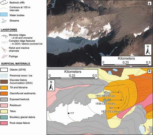
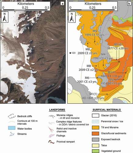
Figure 9. Geomorphological mapping of glacier 121 foreland; (A) aerial orthophotographs (image date 16 September 2016) with 0.25 m spatial resolution showing the glacier foreland, (B) Geomorphological map of area shown in (A) showing the foreland of glacier 121 (Figure 2d) with annotations showing the moraine surveyed for lichenometry and the resulting calculated ages. Map based on field mapping and aerial orthophotographs from 16 September 2016 with 0.25 m spatial resolution

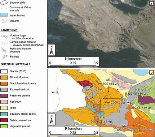
Figure 10. Geomorphological mapping of glacier 123 foreland; (A) aerial orthophotographs (image date 19 September 2011) with 0.25 m spatial resolution showing the glacier foreland, (B) Geomorphological map of area shown in (A) showing the foreland of glacier 123 (Figure 2e) with annotations showing the moraine surveyed for lichenometry and the resulting calculated ages. Note: Map based on field mapping and aerial orthophotographs from 2016 however, due to shading on the 2016 imagery on which the geomorphological map (B) is based, aerial imagery from 2011 (A) is shown

Historical glacier limits in 1952

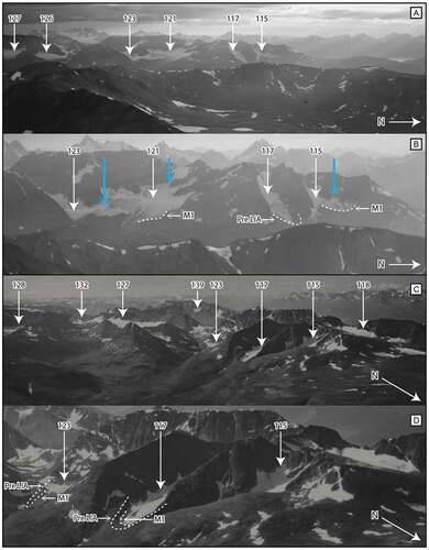
Oblique aerial photographs taken of the field site provide a valuable reference for documenting glacier extent (Figure 11). In 1952, glacier 115 was flowing into the area now occupied by a moraine-dammed lake (formed sometime after 1952 and before 1989 based on the imagery), constrained by the M1 moraine. There was also evidence of confluence with another ice body (Figure 11), which was not verifiable in the field due to a large discrete debris accumulation that either covers any remaining ice or has replaced the ice completely (see Figure 2b). The terminus of glacier 117 is just visible and was not past the large latero-frontal moraine (pre-LIA) that encloses the cirque (Figure 11). The main area of glacier 121 can be seen filling the entirety of the cirque and was confluent with glacier 123 to the southeast, while also being connected to the hanging glacier on the cirque headwall by a narrow ice tongue (Figure 11). The confirmation of these ice bodies being connected in 1952 lends support to the mapping of this uppermost ice body as a glacier, where it had previously been overlooked in glacier inventories. Glacier 123 was not overtopping the bedrock cliffs at its front and was being funneled down the narrow gulley on the true right, where the terminus was obscured (Figure 11). An additional photograph taken the same year from a different angle shows glaciers 117 and 123 and confirms that glacier 117 was within the confines of the M1 moraine and was near the position of the M3 moraine (Figure 11). Glacier 123 was a considerable distance from the M1 moraine, just breaching the bedrock lip behind which it currently lies (Figure 11).

Figure 11. Oblique aerial photographs taken on (A) 8 March 1952 and (C) 31 July 1952 and alongside a zoomed and cropped copy of the aforementioned images (B) and (D). Glaciers are labeled according to the Andreassen, Winsvold, et al. (2012) glacier IDs. The dashed lines outline the visible moraines investigated in this study and the blue arrows in (B) show where glaciers were confluent with adjoining glaciers/ice bodies. Image source: National Library of Norway (2019)

Glacier area changes in northern Troms and western Finnmark

LIA maximum extent—1989/2018

The LIA glacial maximum areal extent was mapped for a subset of fifteen glaciers (Figures 12 and Figures 13) all found within region A of our study area (Figure 1). Results show that since the LIA maximum (dated to between 1814 [±41 years] and 1877 [±34 years]) and 1989, the studied glaciers shrank a total of 3.9 km² (39 percent) and that between LIA maximum and 2018 they shrank a total of 6.9 km² (69 percent). Individual glaciers were between 0.12 km² (54 percent; glacier 115) and 0.56 km² (68 percent; glacier 91) larger during their LIA maximum than in 1989 (Figure 12). The largest percentage change between LIA maxima and 1989 was observed at glaciers 91 and 149, which both exhibited a 68 percent areal reduction, and the smallest percentage change was observed at glacier 121, which shrank only 15 percent over the same period (Figure 12). Overall, mean glacier area reduction from LIA maximum to 1989 (n = 15) equates to approximately 0.26 km² (44 percent) and that from LIA maximum to 2018 equates to approximately 0.46 km² (72 percent). Notably, of the five glaciers that exhibit glacier loss of more than 50 percent between LIA maximum and 1989, all are fronted by at least one proglacial lake (Figure 12). The areal extent (and presumably depth) of these lakes varies between and within forelands, and all lakes are within the extrapolated LIA extent, indicating that at some point during glacier recession they would have been in contact with the glacier.

Figure 12. Comparisons of glacial area change between LIA maximum and 1989/2018

Figure 13. Overview of glacier area change from our Rotsund field site since LIA maximum until 2018 (based on moraine maps and lichenometric dating) and including glacier outlines from 1956 topographic maps. The background image is the Norwegian Mapping Authority N50 Digital Terrain Map (NORGEiBILDER 2019)

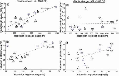
When examining the changes in glacier length for the same glaciers (n = 15), our data indicate that between the LIA maximum and 1989, individual glaciers receded between 1,175 and 52 m (63 and 11 percent, respectively), and between 1989 and 2018 the same glaciers receded between 545 and 77 m (48 and 5 percent respectively). When plotting these reductions in glacier length against the reduction in glacier area over the periods LIA to 1989 and 1989 to 2018 there is a general trend of larger glaciers having experienced greater length reductions (Figure 14).

1907–1989

For some of the larger glaciers (n = 84) there are historical data from 1907, 1952, 1954, 1955, 1956, and 1966 (Figure 15). Comparing the outlines from the historical 1:100,000 and 1:50,000 topographic maps and our satellite image glacier outlines reveals steady glacier area loss throughout the twentieth century across the whole region, with an anomalous increase observed between some of the 1956 and 1989 outlines (Figure 15a, panel V). It should be noted, however, that with the exception of the 1907 and 1966 outlines (from the Øksfjordjøkelen and Langfjordjøkelen ice caps and surrounding area; Figure 15a, panel I), these historical glacier outlines are for different periods and glaciers. When comparing the percentage area change across the data set, there is a pattern of reduction in glacier area throughout the region (Figure 15b). Furthermore, the fifty-nine years between 1907 and 1966 experienced a 9 percent reduction in glacial area, whereas the twenty-three-year period 1966 to 1989 experienced a 12 percent reduction in glacial area (Figure 15b, panel I). Our results therefore indicate that the rate of glacial shrinkage was increasing toward the end of the twentieth century.

1989–2018

In total, 219 glaciers were mapped from the 1989 Landsat 5 satellite imagery, with a total area of 101.8 km² (Table 3). The total number of glaciers includes 78 newly identified and mapped ice bodies that are not included within the most recent edition of the Inventory of Norwegian Glaciers (Andreassen, Winsvold, et al. 2012; Table 3). Of these newly identified glacier units, 23 were classified as certain and the remaining 55 were classified as probable (n = 10) and possible (n = 45; Table 3). The 1989 total area of the Andreassen, Winsvold, et al. (2012) glaciers was 94 km² and the total area of the additional 78 glaciers found in our study was 7.8 km². Of these, the area of certain glaciers was 2.6 km². Additional cloud- and snow-free imagery and/or ground truthing is needed to confirm or reject the glacial status of the 55 probable and possible glaciers.

Table 3. Summary of remotely sensed glacier area measurements and size over the study period for the whole region of investigation

Year	1989	1994	1999	2006	2011	2014	2018
No. of glaciers	219	228	237	243	249	249	252
Total area (km^2)	101.8	96	81.9	81.9	73.7	67.1	66.4
Max. glacier area (km^2)	12.7	12.5	12.4	12.4	12	11.8	11.8
Mean glacier area (km^2)	0.46	0.42	0.35	0.34	0.3	0.27	0.26
No. glaciers ≥0.5 km^2 (%)	18	16	13	12	10	7	8
No. glaciers <0.5 km^2 (%)	82	84	87	88	90	93	92
Total area change (km^2)^a	n/a	−5.8	−14.1	−0.03	−8.9	−6.6	−0.8
Total area change (%)^a	n/a	−6	−15	−0.04	−10	−9	−1
No. of certain glaciers	164	167	163	169	174	179	182
Total area (km^2)	96.6	91.4	79	78.7	71.6	65.2	64.6
Max. glacier area (km^2)	12.7	12.5	12.4	12.4	12	11.8	11.8
Mean glacier area (km^2)	0.59	0.55	0.48	0.47	0.41	0.36	0.36
No. glaciers ≥0.5 km^2 (%)	24	22	19	17	15	10	11
No. glaciers <0.5 km^2 (%)	76	78	81	83	85	90	89
Total area change (km^2)^a	n/a	−5.2	−12.4	−0.28	−7.1	−6.4	−0.64
Total area change (%)^a	n/a	−5	−14	−0.4	−9	−9	−1
No. of probable glaciers	10	9	9	9	11	15	13
Total area (km^2)	1.3	0.81	0.43	0.37	0.37	0.42	0.36
Max. glacier area (km^2)	0.33	0.26	0.2	0.17	0.08	0.04	0.04
Mean glacier area (km^2)	0.13	0.09	0.05	0.04	0.03	0.03	0.03
Total area change (km^2)^a	n/a	−0.52	−0.38	−0.06	0	+0.05	−0.06
Total area change (%)^a	n/a	−39	−47	−14	0	+13	−14
No. of possible glaciers	45	52	65	65	64	55	57
Total area (km^2)	3.9	3.8	2.5	2.8	2	1.5	1.5
Max. glacier area (km^2)	0.3	0.29	0.21	0.21	0.13	0.08	0.07
Mean glacier area (km^2)	0.09	0.07	0.03	0.04	0.03	0.03	0.03
Total area change (km^2)^a	n/a	−0.09	−1.27	+0.31	−0.81	−0.5	+0.03
Total area change (%)^a	n/a	−2	−34	+13	−29	−25	+2

Note. ^aArea change based on the difference between the total area mapped at the previous time step.

Over the period of satellite observed outlines (1989–2018), the total mapped glacial area of northern Troms and western Finnmark has progressively decreased by 35.4 km² (35 percent), from 101.8 km² in 1989 to 66.4 km² in 2018 (Table 3). The largest net loss, in both absolute area and percentage values (n = −14.1 km² and −15 percent), occurred between 1994 and 1999 (Table 3). Because some glaciers fragmented as they shrank, the number of glacier units mapped increased from 219 in 1989 to 252 in 2018 (Table 3). In the study area, forty-eight glaciers (~22 percent) fragmented into two or more individual units over the period of satellite observation (1989–2018). Furthermore, the apparent increase in the number of glaciers over time masks the shrinkage of glacier bodies below our 0.01 km² size threshold; between 1989 and 2018, thirty-six individual glacier units shrank below 0.01 km² and are therefore no longer recorded because they are too small to accurately map from the coarse-resolution Landsat imagery.

Climate data

Climate data show that mean annual temperatures were generally low until the late 1910s, followed by approximately twenty years of rapid temperature increase (~1.4°C) until end of the 1930s (Figure 16a). Subsequent to 1940, there were approximately fifty years of mean annual temperature decrease until the late 1980s, after which a clear mean annual temperature increase emerges through to the present (~1.1°C; Figure 16a). Between 1874 and 2018, summer temperature generally remained constant (Figure 16b). During the same period, winter temperature generally increased until approximately 1940 (from approximately −1.5°C to −0.1°C) and then decreased until the late 1980s before warming again until the present (from approximately −1.3°C to 0.2°C Figure 16c). The year 2007 marks the first time within the records that the ten-year average for winter temperature exceeded 0°C (Figure 16c), with each subsequent year experiencing higher temperatures. Total annual precipitation patterns exhibit a less varied pattern across the observation period (Figure 16a). The winter and summer precipitation values have shown a steady decrease since the early 2000s (Figure 16).

Discussion

Lichenometry and the LIA extent of glaciers within the Rotsund Valley

All of the glacier forelands of the Rotsund Valley have moraines that are accessible and suitable for lichenometry (e.g., blocky and showing minimal evidence of postdepositional reworking). Based on LIA moraine characteristics in similar areas (e.g., Winkler 2003; Baumann, Winkler, and Andreassen 2009; Imhof, Nesje, and Nussbaumer 2012; Weber et al. 2019), the M1 moraines in the Rotsund Valley (Figures 7–10) were initially identified from remote sensing as marking LIA maxima, as indicated by their geomorphology, vegetation coverage, and position within glacial forelands (see section Lichenometry and the LIA extent of glaciers within the Rotsund Valley). Our lichenometry confirms this initial hypothesis: The M1 moraines date to between 1814 (±41 years) and 1877 (±34 years), indicating a nineteenth-century LIA maximum. For the studied glaciers in the Rotsund Valley, it was the glaciers at higher elevations, with additional smaller glaciers/snow patches feeding into them (glaciers 115 and 117; Figures 2 and 11), that achieved an early nineteenth-century LIA maximum. In Norway and other mountain regions worldwide, local-scale asynchronicity in patterns of glacial advance and retreat has been explained by differences in glacier hypsometry, with glaciers at higher elevations reaching their LIA maxima earlier than neighboring glaciers at lower elevations (e.g., Nesje et al. 2008; Chenet et al. 2010; Pratt-Sitaula et al. 2011). One potential factor leading to the apparent asynchronicity in LIA maxima of glaciers in the Rotsund Valley (Table 2) could therefore be explained by glacier hypsometry. Other factors, such as differences in glacier shape, glacier aspect, microclimate, and slope angle, may also play a role in modulating the response of glaciers in the Rotsund Valley to changes in climate (Young et al. 2011; Brugger et al. 2019).

On the forelands of glaciers 117, 121, and 123, a smaller yet well-defined moraine ridge (M2) lies immediately within the M1 moraines (Figures 8–10). The M2 moraines were dated to 1932 (±17 years), 1936 (±16 years), and 1954 (±15 years; Table 2). Though the M2 moraine fronting glacier 123 seems to have formed approximately eighteen to twenty-two years later than the other M2 moraines, we conclude that given that all of the M2 moraines exhibit markedly similar form, position, and vegetation coverage, they result from the same moraine-forming event dating to the early twentieth century (Table 2). The apparent asynchronicity again resulting from differences in glacier characteristics that can modulate individual glacier responses to climate forcing at a local scale (Chenet et al. 2010; Pratt-Sitaula et al. 2011; Brugger et al. 2019). Furthermore, the M2 moraines observed in the Rotsund Valley are comparable with a series of moraines fronting nine glaciers on the nearby Lyngen Peninsula, which have previously been dated to between 1910 and 1935 and subsequently attributed to the LIA maximum (Ballantyne 1990).

The climate data (Figure 16) show that winter precipitation was increased for several years between the late 1890s to the start of the 1910s and that between approximately 1900 and 1920 annual temperature decreased. We suggest that the observed approximately twenty-year period of lowering temperatures coupled with approximately ten years of increased winter precipitation (Figure 16) caused the glaciers of northern Troms to experience a small advance or still stand, during a period of net retreat from the nineteenth-century LIA maximum (M1 moraines; Table 2). Consequently, we suggest that the M2 moraines of the early nineteenth century in our study area of the Rotsund Valley may not document LIA maximum as proposed for the Lyngen Peninsula (Ballantyne 1990). Instead, we conclude that the M2 moraines of the Rotsund Valley were formed during a period of rapid climate variability, initiated in approximately 1880 and continuing throughout the twentieth century.

The remaining moraines, M3 to M8, document a more recent and rapid retreat from the mid-twentieth to early twenty-first century (1955–2009; Table 2). In forelands where numerous moraines are present (e.g., the foreland of glacier 121), topography can be considered as the driving factor behind moraine formation (Barr and Lovell 2014). Shallow glacier beds are likely to result in deposition of smaller, yet more numerous moraines triggered by ice margin fluctuations as a response to minor variations in climate (Barr and Lovell 2014), whereas glaciers in steep cirques are less likely to respond to minor climate variations, leading to more stable margins and fewer, yet larger, moraines (Barr and Lovell 2014). The relatively flat forelands of glaciers 121 and 123 are therefore likely responsible for the more numerous moraines that are present (Figures 9 and 10).

In summary, our results show a nineteenth-century LIA maximum (1814–1877; Table 2), in contrast to the twentieth-century LIA maximum (1910–1930) as proposed for the Lyngen Peninsula (Ballantyne 1990). An early to mid-nineteenth-century LIA maxima in our in northern Troms study area represents a considerably later glacial advance than similar studies from central and southern Norway, which document a mid-eighteenth-century LIA maximum (Nesje [2009] and references therein). The more recent LIA advance found for high-arctic glaciers within Norway compared to central and southern Norway was thought to be the result of a reduction in summer temperate and an increase in winter snowfall, corresponding with a northward retreat of the oceanic polar front during the nineteenth century (Ballantyne 1990).

Comparisons with alternative lichenometric dating curves

We note that the apparent growth rates (section Comparisons with alternative lichenometric dating curves), as calculated from our dating curve (Figure 6), are slower than those reported from elsewhere in Norway (e.g., Erikstad and Sollid 1986; Ballantyne 1990; Winkler 2003). To examine the implications of the variable lichen growth rates for calculated substrate ages, we experimented with three additional curves (Supplementary Figure 1), specifically from the Lyngen Peninsula in Troms county (69° N; Ballantyne 1990), Svartisen and Okstindan in Nordland county (66–67° N; Winkler 2003), and Jostedalsbreen and Jotunheimen in Vestland county (61–62° N; Erikstad and Sollid 1986). The resulting ages for the oldest surfaces resulted in a maximum discrepancy of approximately 142 years (Supplementary Table 1) and the maximum discrepancy for the youngest surfaces was approximately 14 years, with the lag time before initial lichen colonization ranging from 9 to 22 years (Supplementary Table 1). This indicates that the existing lichen growth curves for Norway cannot be employed outside of their original study areas, likely because of the different climatic regimes and their controls on lichen growth rates. Indeed, Beschel (1961) coined the term hygrocontinentality to explain discrepancies in growth rate as a function of different climatic variables across a range of spatial scales (e.g., <100 km to >4,000 km), which has since been verified by a number of lichenometric investigations (e.g., Beschel 1961; Gribbon 1964; Curry 1969; ten Brink 1973; Evans, Archer, and Wilson 1999; Hansen 2010).

The impact of hygrocontinentality or, indeed, climate more generally on lichen growth relates to two primary factors: (1) the amount of effective precipitation and (2) the duration of snow cover (Beschel 1961; Curry 1969; Benedict 1990, 2008; Hamilton 1995; Evans, Archer, and Wilson 1999; Hansen 2010). Because precipitation is known to differ substantially across Norway, with both latitude and longitude, it is the most likely control on variable lichen growth rates. For example, both Jostedalsbreen and Jotunheimen in Vestland and Svartisen and Okstindan in Nordland county are areas of high precipitation greater than 2,000 mm year⁻¹ (potentially exceeding 4,000 mm year⁻¹ depending on specific location; SeNorge 2019), whereas our research in the Rotsund Valley (and the Nordresia region), northern Troms county, is in an area of relatively low precipitation, between 500 and 700 mm year⁻¹ (Supplementary Figure 2a; http://www.senorge.no/index.html?p=klima). The higher precipitation in Vestland and Nordland counties has therefore resulted in not only a difference in the shape of the age–size curve (Supplementary Figure 1) but a considerable difference in the averaged lichen growth rate over the last 210 years. Furthermore, when taking a simple average growth rate over the 210-year period for the four different sites (Jostedalsbreen, Svartisen, Lyngen Peninsula, and the Rotsund Valley) and plotting this against the available local total precipitation values over the period 2007 to 2018, it is clear that areas of higher precipitation result in faster lichen growth rates (Supplementary Figure 2b). For example, the lichen growth rate in Vestland and Nordland counties is three times greater than that in the Rotsund Valley (Supplementary Figure 2b), and even within Troms county, an increase in precipitation across a west to east transect results in the lichen growth rate on the Lyngen Peninsula being around 50 percent greater than that of the Rotsund Valley (Supplementary Figure 2b).

As a result of our investigation into lichen growth as a function of hygrocontinentality (Supplementary Figure 2b), it is apparent that the climate of Norway can substantially impact not only the timing and extent of LIA maximum (as initially outlined by Ballantyne 1990) but also the rates of lichen growth and resulting shape of any age–size curves and calculated surface ages (Supplementary Table 1, Figure 1). We therefore conclude that given the considerably lower precipitation rates across Nordreisa county compared to the Lyngen peninsula (or other sites further south; Supplementary Figure 2a), our site-specific dating curve (Figure 6) remains the most reliable tool for lichenometric dating within the Rotsund Valley.

Changes in glacier size: links with climate and topography

Little Ice Age maxima to late twentieth century

Our LIA reconstructions (Figure 12) cover a small subset of fifteen glaciers within region A (Figure 1). The results show that the reconstructed glacier area decreased from 10 km² at LIA maximum to 6.2 km² in 1989 and to 3.1 km² in 2018 (Figure 12). It is difficult to find a direct comparison of LIA area reconstructions because different studies examine area change over different time frames using different methods (e.g., Andreassen et al. 2008; Stokes et al. 2018). A relatively close comparison can, however, be made to glacier area change in Jotunheimen and Hardangerjøkulen (southern Norway). Between LIA maximum (~1750) and 2003, glaciers in Jotunheimen (n = 233) shrank by approximately 100 km² (35 percent; Baumann, Winkler, and Andreassen 2009), and between LIA maxium (~1750) and 2013 the Hardangerjøkulen ice cap shrank by approximately 40.3 km² (37 percent; Weber et al. 2019). In comparison, our results show a 39 percent reduction in glacier area over a shorter time frame (LIA maxima [~1814] to 1989). Comparatively, results from Langfjordjøkelen in western Finnmark have shown that this ice cap has experienced the highest rates of glacier shrinkage throughout Norway, with a marked reduction in length, area, and glaciological and geodetic mass balance (Andreassen et al. 2020). Indeed, our data on Langfjordjøkelen reveal that glacier area reduced from 10.5 km² in 1989 to 6.8 km² in 2018, representing a 35 percent (3.7 km²) reduction in area over the twenty-nine-year period. Furthermore, recent work analyzing the mass balance of Langfjordjøkelen has shown that between 2008 and 2018 the glacier lost approximately 46 million m³ of ice, firn, and snow, with an accumulated geodetic mass loss of −13.6 m w.e. during the ten-year period (Kjøllmoen 2019). A final comparison is also be made against the study of Nussbaumer, Nesje, and Zumbühl (2011), who also quantified glacier length changes at Jostedalsbreen since LIA maximum (~1750). They found that the Nigardsbreen outlet glacier from the Jostedalsbreen ice cap receded approximately 4,500 m (~29 percent) between LIA maximum and 1990, after which a small, short-lived readvance was recorded (Nussbaumer, Nesje, and Zumbühl 2011). In comparison, the mean reduction in length of the fifteen reconstructed glaciers in our study was approximately 442 m (~33 percent) between LIA maximum (~1814) and 1989, with no readvance recorded during the period of observation.

One substantial trend that was evident in our LIA reconstructions was that all glaciers with area losses greater than 50 percent between LIA maxima and 1989 were fronted by at least one proglacial lake. Ice-marginal proglacial lake development and growth generates a series of positive feedbacks that can accelerate glacier recession, primarily as a result of increased ablation through thermal melting and calving (Carrivick and Tweed 2013). Furthermore, a proglacial lake increases the amount of water at the bed of the glacier, accelerating ice flow velocity, which in turn leads to glacier thinning and increased recession (Carrivick and Tweed 2013). Proglacial lake development in northern Troms appears to be the main driver for some glaciers having experienced greater area reductions since LIA maximum than glaciers terminating on land (Figure 12).

The relationship between absolute reduction in glacier area and glacier length is strongest over the period LIA to 1989 (Figures 14a and 14b). Glaciers that have lost the largest area have, in general, also experienced the greatest length changes. This is not surprising given that most of these were valley glaciers at their LIA maximum and will have experienced most retreat in their lowermost reaches. It is also interesting to note that when only including those glaciers fronted by proglacial lakes (n = 5) the R² values increase to 0.9, suggesting that the development of lakes enhances glacier retreat.

Figure 14. Plots of glacier area and length reduction, as both absolute and percentage values, between the periods (A), (B) LIA to 1989 and (C), (D) 1989 to 2018. Note: The blue circles and corresponding text represent glaciers with at least one proglacial lake within the LIA moraine limits and the numbers represent the individual glacier IDs (Andreassen, Winsvold, et al. 2012)

For the glaciers where historical mapped extents correspond with the Andreassen, Winsvold, et al. (2012) outlines (n = 84; Figure 15), a more detailed examination of glacier change was possible. Overall, glaciers exhibited net retreat during the period 1907 to 1989, broadly in line with that in other areas of northern Norway (e.g., Høgtuvbreen in Nordland and Langfjordjøkelen in Finnmark; Andreassen et al. 2000; Theakstone 2010; Andreason, Kjøllmoen, et al. 2012; Winsvold, Andreassen, and Kienholz 2014). Conversely, in region A of northern Troms, the historical outlines dated to 1956 (n = 12 glaciers) appear to show an increase in glacier area (Figure 15, panel V). Given that no such increase in glacier area for Troms county is reported elsewhere in the literature over this period (1950–1989), coupled with our results showing similar sized glaciers within our study area all exhibiting glacier area loss, it is believed that this apparent increase in glacier area is an artifact of the historical mapping underrepresenting the full extent of glaciers in 1956, leading to an apparent increase in glacier area in 1989.

Figure 15. Comparisons of glacier area change between individual sets of historic outlines (from 1:100,000 Gradteigkart [1907 map] and 1:50,000 Norwegian Mapping Authority topographic maps [1966, 1952, 1954, 1955, and 1956 maps]) and our remotely sensed outlines from 1989. Note: Only the outlines in panel I are overlapping outlines from different time steps; the remaining panels II–V represent glacier outlines from different areas within northern Troms at separate time steps (historic outlines from Winsvold, Andreassen, and Kienholz [2014])

Overall, the larger reduction in glacier area toward the end of the twentieth century represents an increasing rate of shrinkage from 0.2 to −0.5 percent year⁻¹ (Figure 15), which results in a larger shrinkage of glaciers in northern Troms and western Finnmark compared to their southern counterparts. Additionally, our study reveals a greater percentage glacier area reduction, which is attributed in part to the larger proportion of smaller glaciers throughout northern Troms.

1989–2018

The identification and mapping of seventy-eight more glaciers (n = 219) than included within Andreassen, Winsvold, et al. (2012; n = 141) was possible due to the use of multiple overlapping very high-resolution aerial orthophotographs from different time steps (available from NORGEiBILDER 2019). Cross-checking of snow/ice units on aerial orthophotographs (especially those in shadow) was particularly useful when differentiating between a potential very small glacier (<0.5 km²) and a snow patch. The twenty-three additional glaciers classified as certain on the 1989 imagery (Table 3) all show evidence of flowing ice in the form of crevassing and/or ice deformation. The mean size of these twenty-three additional glaciers was only 0.12 km² in 1989, and by 2018 the mean size had reduced to 0.03 km² (a 75 percent reduction). The distribution of the twenty-three additional certain glaciers across northern Troms and western Finnmark shows that very small glaciers in mountain valleys and cirques are most easy to overlook by large-scale glacier inventories; thirteen reside within region A, eight reside within region B, one resides within region C, and the final glacier is a standalone unit in western Finnmark. The remaining glaciers classified as probable and possible in the 1989 imagery (n = 10 and 45, respectively; Table 3) show only partial evidence of glacier characteristics. Additional evidence is needed (i.e., additional snow-free high-resolution imagery or ground truthing), however, before the probable and possible units can be confirmed to be a certain glacier or refuted and reclassified as perennial snow. The importance of mapping such previously unrecorded units has been highlighted by Parkes and Marzeion (2018), who noted that failure to consider uncharted glaciers may be an important cause of difficulties in closing the global mean sea level rise budget during the twentieth century.

The overall net area reduction of glaciers within northern Troms and western Finnmark from 101.8 to 66.4 km² between 1989 and 2018 (Table 3) is in line with the vast majority of reports on glacier change, both regionally and globally (e.g., Andreassen, Winsvold, et al. 2012; Frey, Paul, and Strozzi 2012; Haeberli, Paul, and Zemp 2013; Stokes et al. 2018). The observed glacier shrinkage indicates an approximate reduction in area of approximately 1 percent year⁻¹ between 1989 and 2018, with the largest period of glacier shrinkage between 1994 and 1999 (a net areal reduction of 14.1 km² or 15 percent; Table 3). In contrast, a short period of annual cooling between 1995 and 1999, coupled with increased winter precipitation culminating toward the end of the 1990s, was likely responsible for the period of minimal reduction in glacier area between 1999 and 2006. Overall, our results indicate northern Troms and western Finnmark saw a substantial reduction in glacier area toward the end of the twentieth century.

The lower total area loss recorded between 2006 and 2018 (Table 3) coincided with warmer air temperatures, and this apparent anomaly may be explained by the observed recession and fragmentation of small glaciers into heavily shaded positions (Figure 16). It has been demonstrated that where glaciers do not extend far beyond the shade of a cirque backwall they are likely to receive greater mass inputs (e.g., increased snow from wind drift and/or avalanching) and be more shielded from direct solar radiation (Kuhn 1995; DeBeer and Sharp 2009). In turn, glaciers now situated within deep cirques are likely to have differing responses to climate change than when they were larger or when compared to larger valley and outlet glaciers within the study area (DeBeer and Sharp 2007; Brown, Harper, and Humphrey 2010). There is therefore potential for the retreating glaciers in the mountain belts of northern Troms and western Finnmark to transition into a state of reduced retreat once a critical threshold has been met (in terms of shielding and mass input) and, as a result, they may experience reduced rates of mass loss.

Figure 16. (A) Mean annual temperature, (B) mean summer (June–September) temperature, and (C) mean winter (October–May) temperature. Smoothed dark red and blue lines represent ten-year average; dashed line in (C) represents 0°C. Data recorded in Tromsø from two independent weather stations #90440 and #90450 that have been combined to make a continuous record since 1870 (see section Little Ice Age maxima to late twentieth century; accessed via eKlima 2019)

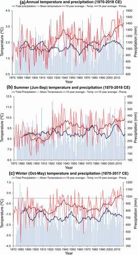
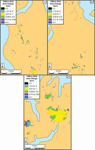
Figure 17. Color-coded map of absolute glacier area change (km²) from 1989 to 2018. Panels 1, 2, and 3 show the predominantly glaciated parts of areas A, B, and, C as outlined in Figure 1

Finally, when examining the relationship between absolute reduction in glacier area and glacier length, it is clear that over the period 1989 to 2018 (Figures 14c and 14d), the correlation is much weaker than that over longer timescales (Figures 14a and 14b); that is, those glaciers that lost a greater absolute area did not always experience a greater length change. This is in contrast to the relationships between the LIA and 1989 (Figures 14a and 14b) and is likely to reflect the transition from a valley-influenced hypsometry to a more upland cirque hypsometry. In the case of the valley-influenced hypsometry, the glacier is more prone to rapid change with a greater proportion of the glacier body below the Equilibrium Line Altitude (ELA). Because many glaciers had a valley-influenced hypsometry at the end of the LIA, the warming in the early twentieth century would have had the greatest effect when their frontal positions were further from the ELA. Subsequently, glaciers receded into more sheltered positions within cirques and their shapes have changed to be more circular, with retreat taking place more evenly around their perimeter.

Glacier size and area change

Our study shows that generally smaller glaciers (e.g., <1 km²) have decreased less in their absolute area (km²) but experienced a larger relative (percentage) reduction (Figures 17 and 18), consistent with findings from other glacierized regions (e.g., Canada: Tennant et al. 2012; Nepal: Ojha et al. 2016; Mongolia: Pan et al. 2018). In northern Troms, glaciers in the central and western mountain belts (regions A and B; Figure 1) have undergone the largest relative reduction in their glacial extent (Figure 18), and the glaciers that were less than 0.05 km² in 1989 experienced the largest percentage loss in glacier area. In contrast, some of the largest glaciers within northern Troms and western Finnmark have experienced absolute area loss of more than 0.5 km² since 1989, with these values only representing a small relative (percentage) reduction in area.

Figure 18. Color-coded map of relative glacier area change (percentage) from 1989 to 2018. Panels 1, 2, and 3 show the predominantly glaciated parts of areas A, B, and C as outlined in Figure 1

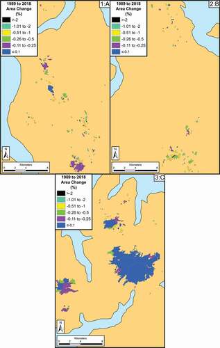
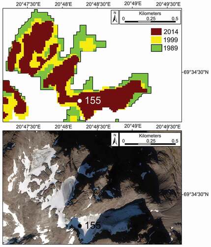
Figure 19. An example of glacier fragmentation over time. (A) Glacier 155 mapped as one unit in 1989. By 1999 it has shrunk and fragmented into two units; the main body and an isolated (glacier) ice patch from its central tongue. In 2014 the glacier had fragmented into three separate units and the ice patch has shrunk below the 0.01 km² size threshold. (B) Aerial orthophotograph (image taken on 16 September 2019 with 0.25 m resolution; NORGEiBILDER 2019) showing glacier 155 in 2016. Note: Though it is possible to discern the very small glacier fragment that shrank below the 0.01 km² size threshold on the aerial imagery (0.25 m resolution), it was not possible to accurately map it on the satellite imagery (15 m resolution)

As glaciers shrink there is also a tendency for them to disintegrate into smaller individual fragments (Paul et al. 2004), and this was observed throughout northern Troms and western Finnmark, with approximately 22 percent of glaciers having fragmented between 1989 and 2018 (Table 3, Figure 19). Glacier fragmentation results in a positive feedback of increased shrinkage, due to the greater perimeter-to-area ratios of glacier fragments compared to larger parent units (Paul et al. 2004). Changes to the localized thermal radiation regime (e.g., increased bedrock exposure lowering surface albedo) results in higher melt rates. Furthermore, where individual glacier fragments become detached from their tributaries, they receive less (possibly no) input (Paul et al. 2004; Jiskoot and Mueller 2012; Carturan et al. 2015). Glacier fragmentation further complicates a glacier’s response to climate change and disproportionately affects those glaciers in exposed and/or low elevation positions.

Future evolution of glaciers in northern Troms and western Finnmark

Climate projections for 2071 to 2100 for Norway indicate a median increase in annual mean air temperature of 4.5°C, with the largest warming occurring in northern Norway (Hanssen-Bauer et al. 2015). Regional temperature predictions for Troms county during the period 2021 to 2050 indicate a median increase in annual temperature of 1.9°C (Hanssen-Bauer et al. 2017). Over the period 2021 to 2050, the precipitation for Troms county is set to increase annually by between 2.7 and 23.2 percent, yet the winter precipitation might either decrease by 6.4 percent or increase by 19.9 percent (Hanssen-Bauer et al. 2017). The greater variance in precipitation predictions highlights the greater uncertainty in future precipitation patterns compared to air temperature changes. Any increase in winter precipitation will, however, be offset by increases in summer temperature that lead to a longer ablation season and higher melt (Stokes et al. 2018). Furthermore, due to increasing temperatures—both annually and seasonally—a higher ratio of precipitation falling as rain is expected (IPCC 2013, 2019; Berghuijs, Woods, and Hrachowitz 2014). Increased rainfall throughout the year can increase surface melting of ice and snow and therefore any increased precipitation is unlikely to mitigate the impacts of temperature increase; hence, glaciers are likely to continue to retreat and/or down-waste (Oltmanns, Straneo, and Tedesco 2019).

For the Langfjord East outlet glacier on the Bergsfjord Peninsula, Andreassen, Kjøllmoen, et al. (2012) suggested that there is a possibility that it will disappear completely within the next 50 to 100 years. Furthermore, glacier recession is most acute for glaciers of less than 0.05 km² at elevations less than 1,400 m a.s.l. (Stokes et al. 2018); as of 2018 these criteria are met for approximately 60 percent of mapped glaciers within northern Troms and western Finnmark. Given that our data set indicates that 71 percent of all mapped glaciers the study area lost more than 50 percent of their area during the period 1989 to 2018, it is plausible that many glaciers in northern Troms and western Finnmark may disappear within the next 50 to 100 years (Nesje et al. 2008; Andreassen, Kjøllmoen, et al. 2012; Andreassen, Winsvold, et al. 2012; Stokes et al. 2018). There is, however, potential for topography to play a role in the preservation of ice bodies that exist in areas of heavy shade and/or debris supply. Glaciers that exist in deep cirques are prone to heavy shading, relatively high mass inputs from snow avalanching and/or wind drift, and increased debris supply (Johnson 1980; Kuhn 1995), which in turn has the potential to decouple them from the climate system (DeBeer and Sharp 2009; Brown, Harper, and Humphrey 2010). The presence of topographically induced glacier–climate decoupling is therefore likely to result in some cirque glaciers being preserved in the future. As a result, there is the possibility that some of these optimally situated ice bodies may outlast the larger glaciers and ice caps located on exposed plateaus, which have no protection from a warming and wetting climate (Hanssen-Bauer et al. 2017; IPCC 2019).

Conclusions

This article presents new data on glacier change throughout northern Troms and western Finnmark, northern Norway, from the LIA maxima to 2018 using lichenometry, historical maps, existing glacier inventories, and new remotely sensed glacier outlines. The LIA maxima for a series of small glaciers in the Rotsund Valley occurred between 1814 (±41 years) and 1877 (±34 years), earlier than has been reported for the larger glaciers on the nearby Lyngen Peninsula. Extrapolation of our LIA reconstructions to eleven other glacier forelands has shown that glaciers were between 15 and 68 percent larger at their LIA maximum than in 1989. Of the fifteen glaciers with LIA reconstructions, all glaciers exhibiting more than 50 percent area loss between the LIA maximum and 1989 are fronted by proglacial lakes within the confines of the LIA maximum moraine.

Analysis of historical maps has shown that throughout the first half of the twentieth century, glacier recession was minimal (~0.2 percent year⁻¹), but between 1966 and 1989 rates of glacier recession more than doubled (~0.5 percent year⁻¹; Figure 15). Implementation of a new glacier identification scoring system, using multiple very high-resolution aerial orthophotographs (0.25 m resolution) to cross-check mapping of coarse-resolution satellite imagery (30–15 m resolution), enabled the identification and mapping of seventy-eight additional glaciers in 1989 (twenty-three of which are classified as certain) that were not included in the Inventory of Norwegian Glaciers (Andreassen, Winsvold, et al. 2012). Over the twenty-nine-year period of satellite observation (1989–2018), we document a 35.4 km² reduction in glacial area (35 percent) within northern Troms and western Finnmark. The greatest glacier area loss occurred between 1994 and 1999, with a net reduction of approximately 2.8 km² year⁻¹ (20 percent year⁻¹) linked to a period of annual warming initiated in approximately 1985. Our analysis has confirmed that it is the very small glaciers (<0.5 km²) that show the highest relative shrinkage, and as of 2018 over 90 percent of glaciers mapped were <0.5 km² in their areal extent (Table 3). Finally, we suggest that where topographical setting permits (e.g., deep shaded cirques), very small glaciers within northern Troms and western Finnmark could outlast the larger ice caps located on the elevated and exposed plateaus.

Data availability

The shapefile data of glacier outlines supporting the findings of this study will be submitted to the Global Land Ice Measurements from Space (GLIMS) initiative.

Acknowledgments

We thank Lexus Norway, who provided a vehicle for JRL to use during fieldwork. JRL thanks Robert Leigh and James Linighan for fieldwork assistance. Landsat 5 TM, 7 ETM+, and 8 OLI imagery were downloaded free of charge from the USGS Earth Explorer website (https://earthexplorer.usgs.gov/), and aerial orthophotographs were kindly provided by the Norwegian Mapping Authority (Kartverket). Prior glacier data as collated by the CryoClim project were also used, including glacier outlines downloaded directly from the Norwegian Water Resources and Energy Directorate (NVE) website (https://www.nve.no/hydrology/glaciers/glacier-data/). Finally, we thank the editors (A. E. Jennings and J. C. Yde) and we are grateful for the comprehensive reviews provided by an anonymous reviewer and Stefan Winkler, who also shared insight and lichenometric data from the Svartisen region of northern Norway.

Disclosure statement

No potential conflict of interest was reported by the authors.

Funding

We acknowledge the IAPETUS DTP and the Alpkit Foundation, whose grants provided JRL funding for fieldwork in northern Troms. JRL is supported by a Natural Environment Research Council UK studentship (NE/L002590/1). This work will also act as a contribution to the project Copernicus bretjeneste (Copernicus Glacier Service Norway, Contract NIT.06.15.5).

Supplementary material

Supplemental data for this article can be accessed on the publisher’s website.

References

- Andreassen, L. M., B. Kjøllmoen, A. Rasmussen, K. Melvold, and Ø. Nordli. 2012. Langfjordjøkelen, a rapidly shrinking glacier in northern Norway. Journal of Glaciology 58 (209):581–93. doi:https://doi.org/10.3189/2012JoG11J014.
- Andreassen, L. M., B. Kjøllmoen, N. T. Knudsen, W. B. Whalley, and J. Fjellanger. 2000. Regional change of glaciers in northern Norway. In NVE report, ed. L. M. Andreassen, Report No. 1, 132. Oslo: Norwegian Water Resources and Energy Directorate. http://publikasjoner.nve.no/report/2000/report2000_01.pdf.
- Andreassen, L. M., F. Paul, A. Kaab, and J. E. Hausberg. 2008. Landsat-derived glacier inventory for Jotunheimen, Norway, and deduced glacier changes since the 1930s. The Cryosphere 2 (2):131–45. doi:https://doi.org/10.5194/tcd-2-299-2008.
- Andreassen, L. M., H. Elvehøy, B. Kjøllmoen, and J. M. Belart. 2020. Glacier change in Norway since the 1960s–an overview of mass balance, area, length and surface elevation changes. Journal of Glaciology 66 (256):1–16. doi:https://doi.org/10.1017/jog.2020.10.
- Andreassen, L. M., M. Huss, K. Melvold, H. Elvehøy, and S. H. Winsvold. 2015. Ice thickness measurements and volume estimates for glaciers in Norway. Journal of Glaciology 61 (228):763–75. doi:https://doi.org/10.3189/2015JoG14J161.
- Andreassen, L. M., S. H. Winsvold, F. Paul, and J. E. Hausberg. 2012. Inventory of Norwegian glaciers, ed. L. M. Andreassen and S. H. Winsvold. Oslo: Norwegian Water Resources and Energy Directorate.
- Armstrong, R. A. 2011. The biology of the crustose lichen Rhizocarpon geographicum. Symbiosis 55 (2):53–67. doi:https://doi.org/10.1007/s13199-011-0147-x.
- Augland, L. E., A. Andresen, D. Gasser, and M. G. Steltenpohl. 2014. Early Ordovician to Silurian evolution of exotic terranes in the Scandinavian Caledonides of the Ofoten–Troms area – Terrane characterization and correlation based on new U–Pb zircon ages and Lu–Hf isotopic data. Geological Society, London, Special Publications 390 (1):655–78. doi:https://doi.org/10.1144/SP390.19.
- Ballantyne, C. K. 1990. The Holocene glacial history of Lyngshalvoya, northern Norway: Chronology and climatic implications. Boreas 19:93–117. doi:https://doi.org/10.1111/j.1502-3885.1990.tb00570.x.
- Barr, I. D., and H. Lovell. 2014. A review of topographic controls on moraine distribution. Geomorphology 226:44–64. doi:https://doi.org/10.1016/j.geomorph.2014.07.030.
- Baumann, S., S. Winkler, and L. M. Andreassen. 2009. Mapping glaciers in Jotunheimen, South-Norway, during the “Little Ice Age” maximum. The Cryosphere 3:231–43. doi:https://doi.org/10.5194/tc-3-231-2009.
- Benedict, J. B. 1990. Experiments on lichen growth. I. Seasonal patterns and environmental controls. Arctic and Alpine Research 22 (3):244–54. doi:https://doi.org/10.1080/00040851.1990.12002788.
- Benedict, J. B. 2008. Experiments on lichen growth, III. The shape of the age-size curve. Arctic, Antarctic, and Alpine Research 40 (1):15–26. doi:https://doi.org/10.1657/1523-0430(06-030)[BENEDICT]2.0.CO;2.
- Berghuijs, W. R., R. A. Woods, and M. Hrachowitz. 2014. A precipitation shift from snow towards rain leads to a decrease in streamflow. Nature Climate Change 4 (7):583–86. doi:https://doi.org/10.1038/nclimate2246.
- Beschel, R. E. 1950. Flechten als Altersmasstab rezenter Moranen. Zeitschrift fur Gletscherkunde und Glazialgeologie 1 (2):152–61.
- Beschel, R. E. 1961. Dating rock surfaces by lichen growth and its application to glaciology and physiography (lichenometry). In Geology of the Arctic, ed. G. O. Raasch, vol. 2, 1044–62. Toronto: University of Toronto Press.
- Bickerton, R. W., and J. A. Matthews. 1993. ‘Little Ice Age’ variations of outlet glaciers from the Jostedalsbreen ice‐cap, southern Norway: A regional lichenometric‐dating study of ice‐marginal moraine sequences and their climatic significance. Journal of Quaternary Science 8 (1):45–66. doi:https://doi.org/10.1002/jqs.3390080105.
- Bonan, D. B., J. E. Christian, and K. Christianson. 2019. Influence of North Atlantic climate variability on glacier mass balance in Norway, Sweden and Svalbard. Journal of Glaciology 65 (252):580–94. doi:https://doi.org/10.1017/jog.2019.35.
- Bradwell, T. 2010. Studies on the growth of Rhizocarpon geographicum in NW Scotland, and some implications for lichenometry. Geografiska Annaler, Series A: Physical Geography 92 (1):41–52. doi:https://doi.org/10.1111/j.1468-0459.2010.00376.x.
- Brown, J., J. Harper, and N. Humphrey. 2010. Cirque glacier sensitivity to 21st century warming: Sperry Glacier, Rocky Mountains, USA. Global and Planetary Change 74 (2):91–98. doi:https://doi.org/10.1016/j.gloplacha.2010.09.001.
- Brugger, K. A., B. Laabs, A. Reimers, and N. Bensen. 2019. Late Pleistocene glaciation in the Mosquito Range, Colorado, USA: Chronology and climate. Journal of Quaternary Science 34 (3):187–202. doi:https://doi.org/10.1002/jqs.3090.
- Calkin, P. E., and J. M. Ellis. 1980. A lichenometric dating curve and its application to Holocene glacier studies in the central Brooks Range, Alaska. Arctic and Alpine Research 12 (3):245–64. doi:https://doi.org/10.2307/1550713.
- Carrivick, J. L., and F. S. Tweed. 2013. Proglacial lakes: Character, behaviour and geological importance. Quaternary Science Reviews 78:34–52. doi:https://doi.org/10.1016/j.quascirev.2013.07.028.
- Carturan, L., F. Cazorzi, F. De Blasi, and G. Dalla Fontana. 2015. Air temperature variability over three glaciers in the Ortles-Cevedale (Italian Alps): Effects of glacier fragmentation, comparison of calculation methods, and impacts on mass balance modeling. The Cryosphere 9 (3):1129–46. doi:https://doi.org/10.5194/tc-9-1129-2015.
- Chandler, B. M. P., H. Lovell, C. M. Boston, S. Lukas, I. D. Barr, Í. Ö. Benediktsson, D. I. Benn, C. D. Clark, C. M. Darvill, D. J. A. Evans, et al. 2018. Glacial geomorphological mapping: A review of approaches and frameworks for best practice. Earth-Science Reviews 85:806–46. doi:https://doi.org/10.1016/j.earscirev.2018.07.015.
- Chenet, M., E. Roussel, V. Jomelli, and D. Grancher. 2010. Asynchronous Little Ice Age glacial maximum extent in southeast Iceland. Geomorphology 114 (3):253–60. doi:https://doi.org/10.1016/j.geomorph.2009.07.012.
- Curry, R. R. 1969. Holocene climatic and glacial history of the central Sierra Nevada, California. Geological Society of America Special Papers 123:1–47. doi:https://doi.org/10.1130/SPE123-p1.
- DeBeer, C. M., and M. J. Sharp. 2007. Recent changes in glacier area and volume within the southern Canadian Cordillera. Annals of Glaciology 46:215–21. doi:https://doi.org/10.3189/172756407782871710.
- DeBeer, C. M., and M. J. Sharp. 2009. Topographic influences on recent changes of very small glaciers in the Monashee Mountains, British Columbia, Canada. Journal of Glaciology 55 (192):691–700. doi:https://doi.org/10.3189/002214309789470851.
- eKlima. 2019. Norwegian Meteorological Institute climate database. Available at: http://www.eklima.no/.
- Erikstad, L., and J. L. Sollid. 1986. Neoglaciation in South Norway using lichenometric methods. Norsk Geografisk Tidsskrift - Norwegian Journal of Geography 40 (2):85–105. doi:https://doi.org/10.1080/00291958608552159.
- Evans, D. J. A., B. R. Rea, J. D. Hansom, and W. B. Whalley. 2002. Geomorphology and style of plateau icefield deglaciation in fjord terrains: The example of Troms-Finnmark, north Norway. Journal of Quaternary Science 17 (3):221–39. doi:https://doi.org/10.1002/jqs.675.
- Evans, D. J. A., C. Butcher, and A. V. Kirthisingha. 1994. Neoglaciation and an early “Little Ice Age” in western Norway: Lichenometric evidence from the Sandane area. The Holocene 4 (3):278–89. doi:https://doi.org/10.1177/095968369400400307.
- Evans, D. J. A., M. Ewertowski, and C. Orton. 2017a. The glaciated valley landsystem of Morsárjökull, southeast Iceland. Journal of Maps 13:909–20. doi:https://doi.org/10.1080/17445647.2017.1401491.
- Evans, D. J. A., M. Ewertowski, and C. Orton. 2017b. Skaftafellsjokull, Iceland: Glacial geomorphology recording glacier recession since the Little Ice Age. Journal of Maps 13 (2):358–68. doi:https://doi.org/10.1080/17445647.2017.1310676.
- Evans, D. J. A., M. W. Ewertowski, and C. Orton. 2019. The glacial landsystem of Hoffellsjökull, SE Iceland: Contrasting geomorphological signatures of active temperate glacier recession driven by ice lobe and bed morphology. Geografiska Annaler: Series A, Physical Geography 101 (3):249–76. doi:https://doi.org/10.1080/04353676.2019.1631608.
- Evans, D. J. A., S. Archer, and D. J. H. Wilson. 1999. A comparison of the lichenometric and Schmidt hammer dating techniques based on data from the proglacial areas of some Icelandic glaciers. Quaternary Science Reviews 18:13–41. doi:https://doi.org/10.1016/S0277-3791(98)00098-5.
- Evans, D. J. A., S. Guðmundsson, J. L. Vautrey, K. Fernyough, and W. G. Southworth. 2019. Testing lichenometric techniques in the production of a new growth-rate (curve) for the Breiðamerkurjökull foreland, Iceland, and the analysis of potential climatic drivers of glacier recession. Geografiska Annaler, Series A: Physical Geography 101 (3):225–48. doi:https://doi.org/10.1080/04353676.2019.1622919.
- Frey, H., F. Paul, and T. Strozzi. 2012. Compilation of a glacier inventory for the western Himalayas from satellite data: Methods, challenges, and results. Remote Sensing of Environment 124:832–43. doi:https://doi.org/10.1016/j.rse.2012.06.020.
- Furunes, T., and R. J. Mykletun. 2012. Frozen adventure at risk? A 7-year follow-up study of Norwegian glacier tourism. Scandinavian Journal of Hospitality and Tourism 12 (4):324–48. doi:https://doi.org/10.1080/15022250.2012.748507.
- Gellatly, A. F., J. E. Gordon, W. B. Whalley, and J. D. Hansom. 1988. Thermal regime and geomorphology of plateau ice caps in northern Norway: Observations and implications. Geology 16 (11):983–86. doi:https://doi.org/10.1130/0091-7613(1988)016<0983:TRAGOP>2.3.CO;2.
- Geological Survey of Norway. 2015. Berggrunn: National bedrock database. Trondheim: Norges Geologiske Undersøkelse.
- Giesen, R. H., L. M. Andreassen, J. Oerlemans, and M. R. Van Den Broeke. 2014. Surface energy balance in the ablation zone of Langfjordjøkelen, an arctic, maritime glacier in northern Norway. Journal of Glaciology 60 (219):57–70. doi:https://doi.org/10.3189/2014JoG13J063.
- Gribbon, P. W. F. 1964. Recession of glacier Tasissarssik A, east Greenland. Journal of Glaciology 5 (39):361–63. doi:https://doi.org/10.3189/S0022143000029130.
- Grove, J. M. 2001. The initiation of the “Little Ice Age” in regions round the North Atlantic. Climatic Change 48 (1):53–82. doi:https://doi.org/10.1023/A:1005662822136.
- Grove, J. M. 2004. Little ice ages : Ancient and modern. 2nd ed. London: Routledge.
- Haeberli, W., F. Paul, and M. Zemp. 2013. Vanishing glaciers in the European Alps. Pontifical Academy of Sciences, Scripta Varia 118:1–9. doi:https://doi.org/10.5167/uzh-83973.
- Hamilton, S. J. 1995. Age determinations of rock glaciers using lichenometry. Unpublished PhD thesis, Queens University, Belfast.
- Hansen, E. S. 2010. A review of lichen growth and applied lichenometry in southwest and southeast Greenland. Geografiska Annaler: Series A, Physical Geography 92 (1):65–79. doi:https://doi.org/10.1111/j.1468-0459.2010.00378.x.
- Hanssen-Bauer, I., E. J. Førland, H. H. Hisdal, S. Mayer, A. Nesje, J. E. Ø. Nilsen, S. Sandven, A. B. Sandø, A. Sorteberg, and B. Ådlandsvik. 2015. Klima in norge 2100 - Kunnskapsgrunnlag for klimatilpasning oppdatert i 2015. Report No. 2/2015, The Norwegian Centre for Climate Services, Oslo.
- Hanssen-Bauer, I., E. J. Førland, I. Haddeland, H. Hisdal, S. Mayer, A. Nesje, A., J. E. Ø. Nilsen, S. Sandven, A. B. Sandø, A. Sorteberg, and B. Ådlandsvik. 2017. Climate in Norway 2100 - a knowledge base for climate adaptation. Report No. 1/2017, The Norwegian Centre for Climate Services, Oslo.
- Harrison, S., N. Glasser, V. Winchester, E. Haresign, C. Warren, and K. Jansson. 2006. A glacial lake outburst flood associated with recent mountain glacier retreat, Patagonian Andes. The Holocene 16 (4):611–20. doi:https://doi.org/10.1191/0959683606hl957rr.
- Humlum, O. 1978. Genesis of layered lateral moraines: Implications for palaeoclimatology and lichenometry. Geografiska Tidsskrift 77:65–72. doi:https://doi.org/10.1080/00167223.1978.10649094.
- Imhof, P., A. Nesje, and S. U. Nussbaumer. 2012. Climate and glacier fluctuations at Jostedalsbreen and Folgefonna, southwestern Norway and in the western Alps from the “Little Ice Age” until the present: The influence of the North Atlantic Oscillation. The Holocene 22 (2):235–47. doi:https://doi.org/10.1177/0959683611414935.
- Innes, J. L. 1983. Development of lichenometric dating curves for Highland Scotland. Transactions of the Royal Society of Edinburgh: Earth Sciences 74:23–32. doi:https://doi.org/10.1017/S0263593300009871.
- Innes, J. L. 1984. The optimal sample size in lichenometric studies. Arctic and Alpine Research 16 (2):233–44. doi:https://doi.org/10.2307/1551075.
- Innes, J. L. 1985. Lichenometry. Progress in Physical Geography 9:187–254. doi:https://doi.org/10.1177/030913338500900202.
- Innes, J. L. 1986. Dating exposed rock surfaces in the Arctic by lichenometry: The problem of thallus circularity and its effect on measurement errors. Arctic 39 (3):253–59. doi:https://doi.org/10.1017/S0032247400032769.
- IPCC (Intergovernmental Panel on Climate Change). 2013. Climate change 2013: The physical science basis, contribution of Working Group I to the Fifth Assessment Report of the Intergovernmental Panel on Climate. Cambridge: Cambridge University Press. doi:https://doi.org/10.1017/CBO9781107415324.
- IPCC (Intergovernmental Panel on Climate Change). 2019. Special report: The ocean and cryosphere in a changing climate. https://www.ipcc.ch/report/srocc/.
- Jackson, M., and G. Ragulina. 2014. Inventory of glacier-related hazardous events in Norway. Norwegian Water Resources and Energy Directorate, Report 83:213. doi:https://doi.org/10.13140/2.1.3462.0480.
- Jansen, H. L., J. R. Simonsen, S. O. Dahl, J. Bakke, and P. R. Nielsen. 2016. Holocene glacier and climate fluctuations of the maritime ice cap Høgtuvbreen, northern Norway. The Holocene 26 (5):736–55. doi:https://doi.org/10.1177/0959683615618265.
- Jiskoot, H., and M. S. Mueller. 2012. Glacier fragmentation effects on surface energy balance and runoff: Field measurements and distributed modelling. Hydrological Processes 26 (12):1862–76. doi:https://doi.org/10.1002/hyp.9288.
- Johnson, P. G. 1980. Glacier-rock glacier transition in the southwest Yukon Territory, Canada. Arctic and Alpine Research 12 (2):195–204. doi:https://doi.org/10.2307/1550516.
- Jomelli, V., D. Grancher, D. Brunstein, and O. Solomina. 2008. Recalibration of the yellow Rhizocarpon growth curve in the Cordillera Blanca (Peru) and implications for LIA chronology. Geomorphology 93 (3–4):201–12. doi:https://doi.org/10.1016/j.geomorph.2007.02.021.
- Jomelli, V., D. Grancher, P. Naveau, D. Cooley, and D. Brunstein. 2007. Assessment study of lichenometric methods for dating surfaces. Geomorphology 86 (1–2):131–43. doi:https://doi.org/10.1016/j.geomorph.2006.08.010.
- Karlén, W. 1979. Glacier variations in the Svartisen area, northern Norway. Geografiska Annaler, Series A: Physical Geography 61 (1):11–28. doi:https://doi.org/10.1080/04353676.1979.11879977.
- Karlën, W., and J. L. Black. 2002. Estimates of lichen growth-rate in northern Sweden. Geografiska Annaler, Series A: Physical Geography 84 (3–4):225–32. doi:https://doi.org/10.1111/j.0435-3676.2002.00177.x.
- Kjøllmoen, B. 2019. Reanalysing a glacier mass balance measurement series - Langfjordjøkelen 2008–2018. NVE Report, Report No. 48/2019, 28. Norwegian Water Resources and Energy Directorate, Oslo.
- Kuhn, M. 1995. The mass balance of very small glaciers. Zeitschrift für Gletscherkunde und Glazialgeologie 31:171–79.
- Leigh, J. R. 2016. Testing the reliability of lichenometric dating in a continental high altitude site: A study in the Austrian Alps. Unpublished master’s thesis, Queen Mary University of London, UK
- Leigh, J. R., C. R. Stokes, R. J. Carr, I. S. Evans, L. M. Andreassen, and D. J. A. Evans. 2019. Identifying and mapping very small (<0.5 km2) mountain glaciers on coarse to high-resolution imagery. Journal of Glaciology 65 (254):873–88. doi:https://doi.org/10.1017/jog.2019.50.
- Lindahl, I., B. P. J. Stevens, and K. B. Zwaan. 2005. The geology of the Váddás area, Troms: A key to our understanding of the Upper Allochthon in the Caledonides of northern Norway. Norges Geologiske Undersøkelse 445 (5):5–43.
- Loso, M. G., and D. F. Doak. 2006. The biology behind lichenometric dating curves. Oecologia 147 (2):223–29. doi:https://doi.org/10.1007/s00442-005-0265-3.
- Loso, M. G., D. F. Doak, and R. S. Anderson. 2014. Lichenometric dating of Little Ice Age glacier moraines using explicit demographic models of lichen colonization, growth, and survival. Geografiska Annaler: Series A, Physical Geography 96 (1):21–41. doi:https://doi.org/10.1111/geoa.12022.
- Matthews, J. A. 2005. “Little Ice Age” glacier variations in Jotunheimen, southern Norway: A study in regionally controlled lichenometric dating of recessional moraines with implications for climate and lichen growth rates. The Holocene 15 (1):1–19. doi:https://doi.org/10.1191/0959683605hl779rp.
- Najafi, M. R., F. W. Zwiers, and N. P. Gillett. 2013. Attribution of Arctic temperature change to greenhouse-gas and aerosol influences. In Climate change 2013: The physical science basis. Contribution of Working Group I to the Fifth Assessment Report of the Intergovernmental Panel on Climate Change. Cambridge: Cambridge University Press. doi:https://doi.org/10.1038/NCLIMATE2524.
- National Library of Norway. 2019. Pictures. Available at: https://www.nb.no/search?q=wider%C3%B8e%20nordreisa&mediaQ25 type=bilder&fromDate=19500101&”toDate=19531231
- Nesje, A. 2009. Latest Pleistocene and Holocene alpine glacier fluctuations in Scandinavia. Quaternary Science Reviews 28 (21–22):2119–36. doi:https://doi.org/10.1016/j.quascirev.2008.12.016.
- Nesje, A., Ø. Lie, and S. O. Dahl. 2000. Is the North Atlantic Oscillation reflected in Scandinavian glacier mass balance records? Journal of Quaternary Science 15 (6):587–601. doi:https://doi.org/10.1002/1099-1417(200009)15:6<587::AID-JQS533>3.0.CO;2-2.
- Nesje, A., J. Bakke, S. O. Dahl, Ø. Lie, and J. A. Matthews. 2008. Norwegian mountain glaciers in the past, present and future. Global and Planetary Change 60 (1–2):10–27. doi:https://doi.org/10.1016/j.gloplacha.2006.08.004.
- Nesje, A., and J. A. Matthews. 2011. The Briksdalsbre Event: A winter precipitation-induced decadal-scale glacial advance in southern Norway in the AD 1990s and its implications. The Holocene 22 (2):249–61. doi:https://doi.org/10.1177/0959683611414938.
- NORGEiBILDER. 2019. Norwegian Mapping Authority. Available at: http://www.norgeibilder.no.
- Nussbaumer, S. U., A. Nesje, and H. J. Zumbühl. 2011. Historical glacier fluctuations of Jostedalsbreen and Folgefonna (southern Norway) reassessed by new pictorial and written evidence. The Holocene 21 (3):455–71. doi:https://doi.org/10.1177/0959683610385728.
- NVE. 2016. Glaciers. Available at: //www.nve.no/hydrology/glaciers/glacier-data/
- Norwegian Mapping Authority N50 Digital Terrain Map. Available at: https://kartkatalog.geonorge.no/metadata/e25d0104-0858-4d06-bba8-d154514c11d2
- Ojha, S., K. Fujita, K. Asahi, A. Sakai, D. Lamsal, T. Nuimura, and H. Nagai. 2016. Glacier area shrinkage in eastern Nepal Himalaya since 1992 using high-resolution inventories from aerial photographs and ALOS satellite images. Journal of Glaciology 62 (233):512–24. doi:https://doi.org/10.1017/jog.2016.61.
- Oltmanns, M., F. Straneo, and M. Tedesco. 2019. Increased Greenland melt triggered by large-scale, year-round cyclonic moisture intrusions. Cryosphere 13 (3):815–25. doi:https://doi.org/10.5194/tc-13-815-2019.
- Overpeck, J., K. Hughen, D. Hardy, R. Bradley, R. Case, M. Douglas, B. Finney, K. Gajewski, G. Jacoby, A. Jennings, and S. K. Lamoureux. 1997. Arctic environmental changes of the last four centuries. Science 278 (5341):1251–56. doi:https://doi.org/10.1126/science.278.5341.1251.
- Pan, C. G., A. Pope, U. Kamp, A. Dashtseren, M. Walther, and M. V. Syromyatina. 2018. Glacier recession in the Altai Mountains of Mongolia in 1990–2016. Geografiska Annaler, Series A: Physical Geography 100 (2):185–203. Taylor & Francis. doi:https://doi.org/10.1080/04353676.2017.1407560.
- Parkes, D., and B. Marzeion. 2018. Twentieth-century contribution to sea-level rise from uncharted glaciers. Nature 563 (7732):551–54. Springer US. doi:https://doi.org/10.1038/s41586-018-0687-9.
- Paul, F., R. G. Barry, J. G. Cogley, H. Frey, W. Haeberli, A. Ohmura, C. S. L. Ommanney, B. Raup, A. Rivera, and M. Zemp. 2010. Guidelines for the compilation of glacier inventory parameters from digital sources. GLIMS:1–23. doi:https://doi.org/10.3189/172756410790595778.
- Paul, F., A. Kääb, M. Maisch, T. Kellenberger, and W. Haeberli. 2004. Rapid disintegration of Alpine glaciers observed with satellite data. Geophysical Research Letters 31 (21):12–15. doi:https://doi.org/10.1029/2004GL020816.
- Paul, F., N. E. Barrand, S. Baumann, E. Berthier, T. Bolch, K. Casey, H. Frey, S. P. Joshi, V. Konovalov, R. Le Bris, et al. 2013. On the accuracy of glacier outlines derived from remote-sensing data. Annals of Glaciology 54 (63):171–82. doi:https://doi.org/10.3189/2013AoG63A296.
- Pendleton, S. L., J. P. Briner, D. S. Kaufman, and S. R. Zimmerman. 2017. Using cosmogenic 10Be exposure dating and lichenometry to constrain Holocene glaciation in the central Brooks Range, Alaska. Arctic, Antarctic, and Alpine Research 49 (1):115–32. doi:https://doi.org/10.1657/AAAR0016-045.
- Pratt-Sitaula, B., D. W. Burbank, A. M. Heimsath, N. F. Humphrey, M. Oskin, and J. Putkonen. 2011. Topographic control of asynchronous glacial advances: A case study from Annapurna, Nepal. Geophysical Research Letters 38 (24):1–6. doi:https://doi.org/10.1029/2011GL049940.
- Racoviteanu, A. E., F. Paul, B. Raup, S. J. S. Khalsa, and R. Armstrong. 2009. Challenges and recommendations in mapping of glacier parameters from space: Results of the 2008 global land ice measurements from space (GLIMS) workshop, Boulder, Colorado, USA. Annals of Glaciology 50 (53):53–69. doi:https://doi.org/10.3189/172756410790595804.
- Rasmussen, L. A. 2007. Spatial extent of influence on glacier mass balance of North Atlantic circulation indices. Terra Glacialis 11:43–58.
- Raup, B., A. Kääb, J. S. Kargel, M. P. Bishop, G. Hamilton, E. Lee, F. Paul, F. Rau, D. Soltesz, S. J. S. Khalsa, et al. 2007. Remote sensing and GIS technology in the Global Land Ice Measurements from Space (GLIMS) Project. Computers and Geosciences 33 (1):104–25. doi:https://doi.org/10.1016/j.cageo.2006.05.015.
- Rea, B. R., and D. J. A. Evans. 2007. Quantifying climate and glacier mass balance in north Norway during the Younger Dryas. Palaeogeography, Palaeoclimatology, Palaeoecology 246 (2–4):307–30. doi:https://doi.org/10.1016/j.palaeo.2006.10.010.
- Roof, S., and A. Werner. 2011. Indirect growth curves remain the best choice for lichenometry: Evidence from directly measured growth rates from Svalbard. Arctic, Antarctic, and Alpine Research 43 (4):621–31. doi:https://doi.org/10.1657/1938-4246-43.4.621.
- SeNorge. 2019. Climate data. Available at: http://www.senorge.no/index.html?p=klima
- Serreze, M. C., and R. G. Barry. 2011. Processes and impacts of Arctic amplification: A research synthesis. Global and Planetary Change 77 (1–2):85–96. doi:https://doi.org/10.1016/j.gloplacha.2011.03.004.
- Solomina, O. N., M. Ivanov, and T. Bradwell. 2010. Lichenometric studies on moraines in the Polar Urals. Geografiska Annaler: Series A, Physical Geography 92 (1):81–99. doi:https://doi.org/10.1111/j.1468-0459.2010.00379.x.
- Solomina, O. N., R. S. Bradley, V. Jomelli, A. Geirsdottir, D. S. Kaufman, J. Koch, N. P. McKay, M. Masiokas, G. Miller, A. Nesje, et al. 2016. Glacier fluctuations during the past 2000 years. Quaternary Science Reviews 149:61–90. doi:https://doi.org/10.1016/j.quascirev.2016.04.008.
- Stokes, C. R., L. M. Andreassen, M. R. Champion, and G. D. Corner. 2018. Widespread and accelerating glacier retreat on the Lyngen Peninsula, northern Norway, since their “Little Ice Age” maximum. Journal of Glaciology 64 (243):100–18. doi:https://doi.org/10.1017/jog.2018.3.
- ten Brink, N. W. 1973. Lichen growth rates in West Greenland. Arctic and Alpine Research 5 (4):323–31. doi:https://doi.org/10.1080/00040851.1973.12003742.
- Tennant, C., B. Menounos, R. Wheate, and J. J. Clague. 2012. Area change of glaciers in the Canadian rocky mountains, 1919 to 2006. Cryosphere 6 (6):1541–52. doi:https://doi.org/10.5194/tc-6-1541-2012.
- Theakstone, W. H. 2010. Glacier changes at Svartisen, northern Norway, during the last 125 years: Influence of climate and other factors. Journal of Earth Science 21 (2):123–36. doi:https://doi.org/10.1007/s12583-010-0011-6.
- Thompson, D. W. J., and J. M. Wallace. 2000. Annular modes in the extratropical circulation. Part I: Month-to-month variability. Journal of Climate 13 (5):1000–16. doi:https://doi.org/10.1175/1520-0442(2000)013<1000:AMITEC>2.0.CO;2.
- U.S. Geological Survey. 2019. EarthExplorer. Available at: https://earthexplorer.usgs.gov/
- Vikhamar-Schuler, D., I. Hanssen-Bauer, and E. Førland. 2010. Long-term climate trends of Finnmarksvidda, Northern-Norway. Oslo: Norwegian Meteorological Institute.
- Weber, P., C. M. Boston, H. Lovell, and L. M. Andreassen. 2019. Evolution of the Norwegian plateau icefield Hardangerjøkulen since the ‘Little Ice Age’. The Holocene 29 (12):1885–905. doi:https://doi.org/10.1177/0959683619865601.
- Whalley, W. B. 2009. On the interpretation of discrete debris accumulations associated with glaciers with special reference to the British Isles. Geological Society Special Publication 320:85–102. doi:https://doi.org/10.1144/SP320.7.
- Whalley, W. B. 2012. Using discrete debris accumulations to help interpret Upland glaciation of the Younger Dryas in the British Isles. In Studies on environmental and applied geomorphology, ed. T. Piacentini, 20. Rijeka: InTech. doi:https://doi.org/10.5772/57353.
- Wiles, G. C., D. J. Barclay, and N. E. Young. 2010. A review of lichenometric dating of glacial moraines in Alaska. Geografiska Annaler, Series A: Physical Geography 92 (1):101–09. doi:https://doi.org/10.1111/j.1468-0459.2010.00380.x.
- Winkler, S. 2003. A new interpretation of the date of the “Little Ice Age” glacier maximum at Svartisen and Okstindan, northern Norway. The Holocene 13 (1):83–95. doi:https://doi.org/10.1191/0959683603hl573rp.
- Winkler, S., H. Elvehøy, and A. Nesje. 2009. Glacier fluctuations of Jostedalsbreen, western Norway, during the past 20 years: The sensitive response of maritime mountain glaciers. The Holocene 19 (3):395–414. doi:https://doi.org/10.1177/0959683608101390.
- Winkler, S., J. A. Matthews, R. A. Shakesby, and P. Q. Dresser. 2003. Glacier variations in Breheimen, southern Norway: Dating Little Ice Age moraine sequences at seven low‐altitude glaciers. Journal of Quaternary Science 18 (5):395–413. doi:https://doi.org/10.1002/jqs.756.
- Winsvold, S. H., L. M. Andreassen, and C. Kienholz. 2014. Glacier area and length changes in Norway from repeat inventories. Cryosphere 8 (5):1885–903. doi:https://doi.org/10.5194/tc-8-1885-2014.
- Wittmeier, H. E., J. Bakke, K. Vasskog, and M. Trachsel. 2015. Reconstructing Holocene glacier activity at Langfjordjøkelen, Arctic Norway, using multi-proxy fingerprinting of distal glacier-fed lake sediments. Quaternary Science Reviews 114:78–99. doi:https://doi.org/10.1016/j.quascirev.2015.02.007.
- Xu, M., J. Bogen, Z. Wang, T. E. Bønsnes, and S. Gytri. 2015. Pro‐glacial lake sedimentation from jökulhlaups (GLOF), Blåmannsisen, northern Norway. Earth Surface Processes and Landforms 40 (5):654–65. doi:https://doi.org/10.1002/esp.3664.
- Young, N. E., J. P. Briner, E. M. Leonard, J. M. Licciardi, and K. Lee. 2011. Assessing climatic and nonclimatic forcing of Pinedale glaciation and deglaciation in the western United States. Geology 39 (2):171–74. doi:https://doi.org/10.1130/G31527.1.