Morphological and wood anatomical traits of Rhododendron lepidotum Wall ex G. Don along the elevation gradients in Nepal Himalayas

ABSTRACT

Though variability in morphological features along the environmental gradients has been extensively studied, less information is available on possible adaptations and trends of anatomical features. We examined the variation in morphological and stem anatomical features of a widely distributed (2,200–5,300 m a.s.l.) Rhododendron lepidotum across elevation gradients in Langtang and Sagarmatha National Parks of Nepal Himalayas. Plant samples in each site were collected from three elevation bands (ca. 3,000, 4,000, and 5,000 m a.s.l.). In both study sites, all morphological features measured had their highest value at the lowest elevation and vice versa. Vessel density of basal stem increased but diameter and area of xylem vessels, and length of vessel element and fiber tracheids decreased as elevation increased. Similarly, height and the number of cells in uniseriate rays and height, width, area, and density of multiseriate rays also decreased toward the highest elevation. However, anatomical features of the ultimate branch did not show any distinct pattern with elevation. Morphological features showed more plasticity than anatomical features along the elevation gradients. Decreased plant height, individual leaf area, specific leaf area, and the existing trade-off relationship between vessel diameter and density could have supported a wide distribution of R. lepidotum in Nepal Himalayas.

KEYWORDS:

• Adaptation
• alpine habitat
• plant functional traits
• specific leaf area
• trade-off relationship

Introduction

Structural and functional plasticity and/or adaptive strategies become critical for the growth and survival of plants at high elevations (Körner 2003). Such structural variation allows a plant to enhance its fitness for the successful establishment in cold temperature, short growing season, snowfall, and limited nutrient availability in high-elevation ecosystems (Körner 2012). Structural modifications by plants in alpine ecosystems show highly varying patterns. For instance, with an increase in elevation in high mountain areas, plant height, stem diameter, leaf area, and specific leaf area (SLA) decrease (Oberhuber 2004; Körner 2012; L. Zhang et al. 2012). Leaf area also decreases in stressed conditions (low water, temperature, nutrient supply; Givnish 1987; Pickup, Westoby, and Basden 2005). Leaves with lower SLA are effective in resource-poor, low-temperature, and low-soil-moisture conditions (Reich et al. 1999; Körner 2012). In addition, dwarf plants have a higher chance of surviving low temperatures, snowfall, and wind intensity (Körner 2012). Therefore, one may expect that plants at higher elevations are smaller with thick and small leaves because of the stressful environment, whereas at a lower elevation, where the environment is less stressful, they produce larger and thinner leaves than they do at higher elevations (Körner 2012; L. Zhang et al. 2012; W. Liu, Zheng, and Qi 2020).

Xylem mainly transports water and nutrients from the soil to stem and leaves and also plays an essential role in mechanical support and storage of water, minerals, and carbohydrates. The water transportation is mainly done by specialized xylem conduits, and xylem parenchyma cells are the primary means of radial transport and storage of reserve materials such as starch, fats, and minerals (Myburg, Lev-Yadun, and Sederoff 2013). Any variation in such plant anatomical features reflects changes in environmental conditions and carries unique ecological information related to water and mineral storage, transportation, and mechanical support in plants (Schweingruber 2007).

Xylem conduits vary with stem length, lineage, habit, and climate (Anfodillo, Petit, and Crivellaro 2013; Olson et al. 2014) and are also correlated with elevation and ontogeny (Noshiro and Suzuki 2001; Noshiro, Ikeda, and Joshi 2010; Pathak et al. 2018), and the variation in ray fractions is found to be correlated with temperature, growth form (Morris et al. 2016), and elevation (Noshiro, Ikeda, and Joshi 2010). Plants grown in wet conditions generally have wider conduits than in those growing in comparatively drier conditions (Carlquist and Hoeckman 1985). Wider conduits are much more efficient than narrow conduits, but increased conduit diameter decreases safety under drought stress and freezing-induced cavitation (Tyree and Zimmermann 2002; Chave et al. 2009) because they are more vulnerable to breaking off the conductive stream and blockage by a gas embolism (Hacke et al. 2006; Christman, Sperry, and Adler 2009). The hydraulic architecture of plant stems plays a crucial role in the trade-off of plant functions balancing water and nutrient supply against mechanical stability while minimizing xylem dysfunction by cavitation (Baas et al. 2004). Therefore, we hypothesized that vessel size decreases with an increase in elevation, and to maintain the hydraulic efficiency in comparatively colder climatic conditions at high elevation, the reduced vessel size is compensated by the production of a higher number of vessels per unit area.

Rhododendron species (Ericaceae) of the Nepal Himalayas have a wide variation in growth form (miniature shrub to a giant tree) and habitat (subtropical to nival regions; Milleville 2002) and provide opportunities to explore how morphological and anatomical features vary with growth form and habitat. A few studies examining inter- and intraspecific variation have revealed that wood anatomical features of Rhododendron species are correlated to elevation and ontogeny (diameter and height of plant; Noshiro, Joshi, and Suzuki 1994; Noshiro and Suzuki 1995, 2001; Noshiro, Ikeda, and Joshi 2010; Pathak et al. 2018). To further explore this interface, we selected a shrub species Rhododendron lepidotum Wall. ex G. Don. which has the widest elevational distribution (2,200 to 5,300 m a.s.l.) among the Rhododendron species found in the Nepal Himalayas. Here, we aimed to answer the two following questions: (1) How do morphological and anatomical features of a species having an exceptionally wide distribution range vary along the elevation gradient? and (2) Which features are relatively plastic or static in response to changing elevation? Evidence shows a progressive warming trend in the Himalayan regions than in the lowlands of Nepal (Shrestha and Aryal 2011), and it is expected that along with rising temperatures, average precipitation will also increase in the future (Ministry of Forests and Environment 2019). Thus, this study aimed to better (1) understand the strategies deployed by a widely distributed species to withstand low temperature and (2) predict the probable responses of the species to future climate changes.

Materials and methods

Study species

Rhododendron lepidotum Wall. ex G. Don. (Bhale Sunpatee in Nepali) is an evergreen shrub growing throughout Nepal from 2,200 to 5,300 m a.s.l. covering warm temperate to nival regions (B. B. Shrestha, pers. obs. in Sagarmatha National Park). The natural distribution range of this species includes Nepal, China (Sichuan, Xizang, and Yunan), India (Himalayan states), Bhutan, and Myanmar. The height of the plant ranges from <10 cm in nival regions to >1.5 m at low elevations. It is a resinous shrub with pink, dull purple, or pale yellow flowers often with darker spots and obovate, obovate–elliptic, or oblong–lanceolate leaves (Milleville 2002). At high elevations, it can be found in open grasslands in association with R. setosum, R. anthopogon, and other dwarf plant species. At low elevations (<4,000 m a.s.l.), it is dominant in open areas with full access to sunlight such as along trails and in forest gaps and avoids dense forest canopy (Milleville 2002; Rajbhandari and Watson 2005).

Sampling areas and sample collection

Samples were collected from two national parks located in the Himalayas: Langtang National Park (LNP; 1,710 km²) in central Nepal and Sagarmatha National Park (SNP; 1,148 km²) in eastern Nepal (Figure 1; Supplement 1). The elevation of LNP ranges from 790 to 7,245 m a.s.l. (Mt. Langtang Lirung) with vegetation types encompassing hill sal (Shorea robusta) forests to upper alpine meadows and the elevation of SNP ranges from 2,845 to 8,848 m a.s.l. (Mt. Everest) with vegetation including oak (Quercus spp.) forests in the lower forested zone to the upper alpine meadows with lichens and mosses (Bhuju et al. 2007). Among these two study sites, LNP represents relatively a moist area with annual precipitation 2,085 mm (Department of Hydrology and Meteorology 2013; Supplement 2), whereas SNP represents a semi-arid region with annual precipitation ranging from 425 mm at Lobuche (Pyramid International Laboratory at 5,050 m a.s.l.) to 860 mm at Namche Bazar (3,560 m a.s.l.; Vuillermoz et al. 2008; Supplement 3). At both sites, about 80 percent of the precipitation falls in the monsoon season from June to September.

Figure 1. Map of Nepal showing sample collection sites in Langtang National Park (LNP) and Sagarmatha National Park (SNP).

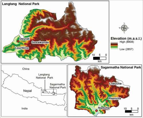
Samples of Rhododendron lepidotum were collected from three different elevations (ca. 3,000, 4,000, and 5,000 m a.s.l.) in LNP and SNP (Figure 1; Supplement 1). At the sampling site in LNP, the uppermost distribution limit of R. lepidotum was 4,460 m a.s.l.; therefore, samples were collected from 4,460 m a.s.l. instead of 5,000 m a.s.l. The collection sites were exposed rocky slopes except at Deurali (3,000 m a.s.l., LNP), where it was in the forest edge. At each sampling site, healthy and tall plants (n = 10) from the southern aspect with no sign of disease and disturbance were cut at the soil surface and transported to the laboratory for further analysis.

Morphological features

Plant height (cm) and internodal length (cm) were measured using a measuring tape and basal and ultimate branch diameters were measured using an Aerospace 0–150 mm digital caliper. For the leaf area (cm²) measurement, the 130 largest and healthy leaves (thirteen from each sample) were selected from samples collected from each elevation band. Because leaves were small in size, the millimeter grid technique was used for measurement of the leaf area (Cornelissen et al. 2003). We placed the leaves on a sheet of paper with a millimeter grid and a drawing of the leaves was made. Then we counted the number of grids and calculated the leaf area by multiplying the number of grids by the grid area. After area measurement, the leaf samples were oven-dried at 60°C for 72 h to determine dry biomass (g). SLA (cm².g^–1) was calculated as the projected leaf area per unit oven-dry mass (Cornelissen et al. 2003).

Anatomical features

Altogether we collected 120 stem wood samples (ten basal and ten ultimate branch stem samples for each of the three elevation bands in two study areas). For stem anatomical analysis, approximately 2-cm-long sections of the basal stem and ultimate branch were excised and stored in 50 percent ethyl alcohol solution until laboratory work began. Thin (15 µm) transversal (sixty basal and sixty ultimate branch stem samples) and tangential (sixty basal stem samples) sections were prepared using a sliding microtome (RMT-45, Radical Instruments) and preserved in 50 percent ethanol. Because of their smaller diameter, we could not obtain thin tangential microsections from the wood samples of the ultimate branches. Thus, we only prepared transversal sections and did not analyze the ray parenchyma features in the ultimate branches. The microsections were stained with 1 percent Safranin for 5 min, washed with an ascending series of ethanol (50, 70, and 90 percent), and finally stained with Fast Green for 2 min. Then the sections were again washed sequentially in ethanol (90 and 100 percent) and xylene and permanently mounted with dibutylphthalate polystyrene xylene (Cutler, Botha, and Stevenson 2008). We cut five tangential sections per basal stem wood sample; the best thin microsection was permanently mounted for ray analysis and the remaining were macerated. For ultimate branch wood samples, small, manually cut wood chips (sixty) were macerated. The sections were macerated for about 10 to 12 h in Jeffrey’s solution (Johansen 1940), washed two to three times with distilled water, and stained with Safranin. Then, semipermanent slides were made using glycerol for the measurement of vessel element and fiber tracheid length. Photographs of prepared sections were taken using a digital microscope (BIO2B microscope with a BEL 89/336 BIO2B camera) with the calibrated scale on ocular, and measurements were done using an image analysis software ImageJ (Rasband 2020).

Xylem vessels were analyzed in transversal sections and ray parenchyma in tangential sections. The macerated tangential sections were used for measurement of vessel element length and fiber tracheid length. All anatomical features were measured randomly except that xylem vessels near the pith and vascular cambium were excluded for the measurement of xylem vessels in transversal sections. Xylem vessel diameter, uniseriate ray height, and uniseriate cell number in each sample were analyzed as the mean of the diameter of sixty vessels/rays observed in three microscopic fields (twenty in each with a field area of 0.1238 mm²). The diameter of each xylem vessel was, in turn, calculated as the mean of radial and tangential diameters of each vessel. Similarly, vessel density and uniseriate ray density were calculated by counting each feature in the microscopic field with an area of 0.1238 mm². The vessel area for each wood sample was calculated using ImageJ and averaged from sixty vessels. Contrary to the uniseriate rays, there were only a few multiseriate rays; therefore, all rays present in the microscopic field (area = 1.6862 mm²) were measured to determine multiseriate ray height, multiseriate ray width, multiseriate ray density, and multiseriate ray area. Vessel element length and fiber tracheid length of each sample were obtained as the mean length of thirty vessel elements and fiber tracheids, respectively, from three microscopic fields (ten in each field with a field area of 0.1238 mm²). In addition, the xylem vulnerability index, which is considered as a measure of xylem safety from embolism, was calculated using the following formula (Carlquist 1977): Vulnerability index = Average vessel diameter/number of vessels/mm².

To explore the effect of axial path length on the stem anatomical features, we followed data standardization procedures described by Lechthaler et al. (2018). Because of the lack of anatomical data in different distances from the apex, we did not explore variation within each plant. Instead we combined data for ten plant samples from the same elevation and explored the variation explained by the axial path length on the basal stem anatomical features in each of three elevations in both study areas. We used type II linear regression with a reduced major axis. With the exception of vessel diameter at 5,000 m a.s.l., uniseriate ray height and cell number at 4,000 m a.s.l. in LNP and vessel density, vessel element length at 3,000 m a.s.l., and uniseriate ray cell number at 5,000 m a.s.l. in SNP, other regression models were not statistically significant (Supplement 9). Due to this inconsistency, we did not use the slope of the regression model to standardize the basal stem anatomical features.

Statistical analysis

The mean values of morphological and anatomical features in three different elevations were compared using a one-way analysis of variance (ANOVA). Prior to ANOVA, a test for homogeneity of variance was conducted. Log10 transformations (all anatomical features and internodal length in SNP) or square root transformations (basal diameter and internodal length in LNP and plant height in SNP) were performed for the variables that did not meet this assumption. Those data that did not meet the assumption of homoscedasticity even after transformation were compared by a nonparametric Kruskal-Wallis test. For multiple pairwise comparisons, ANOVA was followed by Bonferroni tests and the Kruskal-Wallis test was followed by by the Mann Whitney U test. Multiseriate rays were not present in all samples; therefore, only the mean value of all multiseriate ray features was calculated. The sample size of the leaf area was greater than thirty; hence, z-tests were used to compare among elevation bands in each area. All statistical tests were performed in R version 4.0.2 (R Core Team 2020). Overall change in percentage from 3,000 to 5,000 m a.s.l. was calculated using the following formula: Change in each attribute (%) = (value at 3,000 m a.s.l. − value at 5,000 m a.s.l.) × 100/value at 3,000 m a.s.l.

Results

Variation in morphological features

Variation in morphological features was similar in both study sites and the mean values of all morphological features were significantly different (p < .05; Supplement 4). Plants were smaller with a low basal diameter and internodal length at higher elevation (Figure 2). Similarly, both leaf area and SLA decreased with increasing elevation. There was a more pronounced reduction in height (decreased by 75 percent) compared to stem diameter (decreased by 51 percent) toward higher elevations. The leaf area showed more variability, followed by internodal length and plant height, though the SLA varied the least along the elevation gradients. The leaf area at the highest elevation was just 10 percent (i.e., 90 percent reduction) of the leaf area at the lowest elevation in both sites (Figure 2; Supplement 4). However, the SLA at the highest elevation was 75 percent (i.e., 25 percent reduction) of the SLA at the lowest elevation.

Figure 2. Violin plots with Bonferroni pairwise comparisons showing the differences in morphological features between the three elevation zones in LNP and SNP. Within three elevation zones in LNP and SNP, features that do not share the same alphabet have significantly different values (p < .05). See Supplement 4 for details of statistical analyses.

Anatomical features

General anatomical features

The wood was “diffuse-porous” and the vessels were mostly distributed evenly. The vessels were mostly solitary, though sometimes in clusters of two, three, or more (Figure 3). They were polygonal in outline and the radial diameter (15.91 ± 0.30 µm) was greater than the tangential diameter (13.65 ± 0.28 µm; n = 60, p < .05, Z = 5.31). The mean vessel area was 284 ± 82 µm² (n = 3,600).

Figure 3. Transverse sections of a (A), (C) basal stem and (B), (D) ultimate branch collected from LNP (A and B, sample LC10) and SNP (C and D, sample SN6). V = xylem vessel, R = ray parenchyma, FT = fiber tracheid, RB = growth ring boundary, and P = pith.

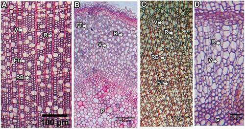
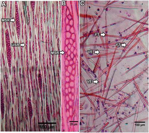
Rays were heterogeneous, dominated by uniseriate rays with one to twenty-one cells in each ray, which were elongated and upright (Figure 4). Multiseriate rays were a few (0–6 in 0.25 mm²); they were absent in two samples from LNP (one each from 4,000 and 5,000 m a.s.l.) and five samples from SNP (four from 5,000 m a.s.l. and one from 4,000 m a.s.l.). Growth rings were distinct in about one-fourth of the samples (eight to thirteen rings) and inconspicuous in the others. The ring boundary was defined by one- to four-layer flattened fiber tracheids developed at the end of the growth period (Figure 3).

Figure 4. (A), (B) Tangential section and (C) macerated sample of a basal stem. MSR = multiseriate rays, USR = uniseriate rays, VE = vessel elements, FT = fiber tracheids.

Variation in basal stem anatomy along elevation gradients

Similar to the morphological features, basal stem anatomy showed a distinct pattern of variation in both study sites. Vessel diameter, vessel area, vessel element length, and fiber tracheid length decreased but vessel density increased with an increase in elevation (Figure 5; Supplements 5 and 6). The height and number of cells in uniseriate rays decreased and multiseriate rays became smaller and sparser toward higher elevations (Figure 6).

Figure 5. Violin plots with Bonferroni pairwise comparisons showing the differences in anatomical features of basal stems between the three elevation zones in LNP and SNP. Within three elevation zones in LNP and SNP, features that do not share the same alphabet have significantly different values (p < .05). See Supplements 5 and 6 for details of statistical analyses.

Figure 6. Variation in multiseriate ray features in the samples collected from LNP and SNP.

Stem anatomical features were less plastic compared to morphological features. In samples collected from the LNP (central Nepal), the height of uniseriate rays and vessel diameter at the highest elevation were 42 and 22 percent lower, respectively, than in the samples from the lowest elevation. Similarly, vessel density and vessel area in the samples from the highest elevation were 80 and 39 percent lower, respectively, than in the samples collected at the lowest elevation in the SNP (eastern Nepal). Vulnerability index values at the highest elevation in the LNP and SNP were 40 and 59 percent lower than at the lowest elevation, respectively, suggesting that vessels at higher elevations were less vulnerable to embolism (Figure 5; Supplement 5).

Variation in ultimate branch anatomy

In contrast to basal anatomy, the ultimate branch anatomy did not show any distinct pattern of variation with elevation. Only values for vessel element length in SNP was significantly different (ANOVA, p < .05; Figure 7; Supplements 7 and 8). Compared to basal diameter, vessels were smaller and denser in the ultimate branch, whereas the length of vessel elements and fiber tracheids was nearly equal (Supplements 7 and 8).

Figure 7. Violin plots with Bonferroni pairwise comparisons showing the variation in anatomical features of the ultimate branch in three elevation zones of LNP and SNP. Different elevations that do not share the same alphabet within LNP and SNP have significantly different values (p < .05). See Supplements 7 and 8 for details of statistical analyses.

Discussion

In this research, we explored the extent to which leaf features, plant height, basal stem, and ultimate branch anatomical traits were influenced by elevation and assessed whether the pattern of their variation was similar in two study sites that differ in precipitation. Most of the studied morphological and wood anatomical features showed variation, with a distinct pattern along the elevation gradient, suggesting the adaptive modifications of R. lepidotum to withstand adverse climatic conditions at higher elevations.

Morphological features along the elevation gradients

Morphological features of R. lepitodum measured in the present study suggests adaptations to harsh conditions at high elevations, such as low temperatures, high wind exposure, and low nutrient and soil moisture availability. Low temperature, shorter growing season, and other climatic extremes hinder the growth and development of plants at high elevations (Körner 2012). The decline in plant height, basal diameter, and internodal length with an increase in elevation (Figure 2) have been also reported for Metrosideros polymorpha, Piea abies, and other plant species (e.g., Cordell et al. 1998; Oleksyn et al. 1998; Kronfuss and Havranek 1999; Hertel and Wesche 2008). Furthermore, greater reduction in the height of R. lepidotum than in stem diameter toward high elevations (Supplement 4) is expected because the upper parts experience colder conditions than the lower parts and vertical growth becomes increasingly constrained (Bernoulli and Körner 1999; Li, Yang, and Krauchi 2003; Körner 2012). The slow growth rate at high elevations might be accompanied by a higher allocation of photosynthate to roots than shoots (Ledig, Bormann, and Wegner 1970; Körner and Renhardt 1987; Oleksyn et al. 1998). Reduced plant height toward higher elevations becomes advantageous in areas with low temperature, high snowfall, and high wind speed because it helps the plant to decrease tissue damage by maintaining high thermal and aerodynamic resistance (Körner 2003, 2012). Shorter height is also beneficial against winter embolism because of the narrower conduits, which are less vulnerable to conduction-blocking embolisms than wider conduits in taller plants (Olson et al. 2018).

Lower leaf area and SLA at higher elevations (Figure 2) were also adaptational and have been observed in other species such as Nothofagus menzisii, ericaceous dwarf shrubs, Ranunculus spp. (Körner, Bannister, and Mark 1986), Metrosideros polymorpha (Cordell et al. 1998), evergreen broad-leaved trees (Tang and Oshawa 1999), tree species of montane rain forest (Velazquez-Rosas, Meave, and Vazquez-Santana 2002), Polylepis forest (Hertel and Wesche 2008), tropical montane forests (van de Weg et al. 2009), and Bergenia purpurascens (L. Zhang et al. 2012). This shows that leaves are in general smaller and thicker at higher elevations. Reduction in leaf size and an increase in thickness can enhance the mechanical strength to withstand stressful environments such as low temperature and high wind at high elevation (Lütz 2010). SLA is negatively correlated with leaf life span (Reich, Walters, and Ellsworth 1997; Wright et al. 2004; Luo, Luo, and Pan 2005). A reduction in SLA of R. lepidotum toward high elevation (Figure 2) therefore may lead to a longer leaf life span. Longer leaf life span can be a useful strategy for plants in cold temperatures to prolong the mean residence time of nutrients such as nitrogen (Escudero et al. 1992; Eckstein, Karlsson, and Weih 1999). However, how leaf life span changes within species of Rhododendron along the elevation gradient in the Himalayas remains unknown and can be a topic for future research.

Anatomical variation along the elevation gradients

Similar to the morphological features, most of the studied anatomical features of R. lepidotum varied with a distinct pattern along the elevation gradients. Vessels were smaller and denser toward higher elevations (Figure 5), a pattern reported previously in Illicium (Carlquist 1982), woody Southern Californian flora (Carlquist and Hoeckman 1985), Alnus nepalensis (Noshiro, Joshi, and Suzuki 1994), Rhododendron spp. (Noshiro, Suzuki, and Ohba 1995), and Metrosideros polymorpha (Fisher et al. 2007). Baas and Carlquist (1985) found more numerous vessels in xeric plants, which is in line with our observation, because high-elevation habitats are more xeric than low-elevation habitats in both of our study sites. However, some species in other studies showed a different pattern. For example, Noshiro and Suzuki (1995) reported that vessel density and size did not vary significantly with elevation in R. anthopogon (3,380–4,950 m a.s.l.) and R. campanulatum (2,790–4,140 m a.s.l.). They also reported an increase in vessel density at higher elevations without significant changes in vessel size in R. lepidotum and R. arboreum. In contrast, vessel diameter and the number of vessels decreased with an increase in elevation in Symphoricarpos microphyllus and vessel diameter decreased up to the middle of the gradient and increased at the end (2,949–3,952 m a.s.l.) in Alchemilla procumbens and Lupinus montanus (Jiménez-Noriega et al. 2017). Such variability among species in the Jiménez-Noriega et al. 2017 study could have been due to different sampling methods, because the wood samples of S. microphyllus were collected from the widest branch at the ground level but wood samples of A. procumbens and L. montanus were collected from the stem below the soil surface. Therefore, vessel features may vary according to life form, location of stem sample relative to soil surface, habitat, and change in environmental conditions rather than showing a consistent pattern of variation.

The functional significance of smaller but denser vessels at a higher elevation can be explained in terms of increased safety from embolism from freeze–thaw cycles (Carlquist 1982; Hacke and Sperry 2001; Fisher et al. 2007) because narrow vessels are less vulnerable to embolism than wider vessels (Carlquist 1982; Chave et al. 2009). Additionally, increased vessel density may compensate for the low conductive efficiency of narrow vessels (Tyree and Zimmermann 2002; Chave et al. 2009; Gea-Izquierdo et al. 2013). Therefore, the hydraulic conductivity of R. lepidotum lost at high elevations as a result of reduced vessel size might have been restored partially due to an increase in vessel density. The lower value of the vulnerability index of R. lepitodum at higher elevations further indicated that stems at high elevations are adapted to low available moisture and low temperature and are less vulnerable to embolism. Air temperature at 3,000 and 5,000 m a.s.l. differs by nearly 11°C and the growing season length decreases by almost 170 days (Bhattarai, Vetaas, and Grytnes 2004). Therefore, the variability in vessel features of R. lepidotum can be a consequence of a shorter growing season and/or an adaptation to the frequent freeze–thaw cycles and low temperature at high elevations.

The shorter vessels and fiber tracheids in R. lepidotum at a higher elevation (Figure 5) is in line with earlier reports for different species (Baas, Werker, and Fahn 1983; Noshiro, Joshi, and Suzuki 1994; Noshiro, Suzuki, and Ohba 1995). Short vessel elements are adaptive to arid conditions because they better localize air embolisms (Carlquist 2001). The decrease in vessel element length was sharp in tree species and gentle in shrub species of Rhododendrons (Noshiro, Suzuki, and Ohba 1995). This trend seems to be related to low temperatures and a shorter growing season, which influence the ontogenesis of the wood (Noshiro and Suzuki 2001). However, X. Zhang, Deng, and Baas (1988) found an increase in the length of vessel element and fiber tracheid with increasing elevation in Syringe oblata var. giraldii. Similarly, in the R. arboreum collected from central and eastern Nepal, the vessel element length and fiber tracheid length were not influenced by elevation and plant size (Noshiro and Suzuki 1995), but these features were strongly associated with elevation in Rolwaling, central Nepal (Noshiro, Ikeda, and Joshi 2010).

Rays in wood facilitate radial transportation and store water, plant hormones, and minerals (Lev-Yadun and Aloni 1995). These rays were smaller and sparser at a high elevation (Figures 5 and 6), which implies that the proportion of living cells decline with elevation. In a study examining twenty-six species of Rhododendron, multiseriate ray area, ray height, and ray width were reported to decrease with increasing elevation (Noshiro, Suzuki, and Ohba 1995). A decrease in multiseriate ray density with increasing elevation has been also reported in R. lepidotum (Noshiro and Suzuki 1995). Ray density gradually decreases with elevation, whereas ray height decreases toward extremes of the elevation gradient in Ribes ciliatum (Jiménez-Noriega, Terrazas, and Lopez-Mata 2015). It appears that a decrease in ray size and density in wood with increasing elevation is a common pattern that may help to withstand severe environmental conditions for survival and evolution of the species at higher elevations (Noshiro, Ikeda, and Joshi 2010).

As discussed above, most of the anatomical features analyzed varied consistently with elevation, indicating adaptational significance. However, the variation in anatomical features of ultimate branches did not follow any consistent pattern with elevation. The reason for this is presently unclear, but it may be related to developmental variation along the axis with comparatively young wood in the ultimate branch, because immature wood shows inconsistency in vessel features (Noshiro and Suzuki 2001).

In addition, independent of growth form, xylem conduit diameter scales with stem length across angiosperm lineages, habits, climates (Anfodillo, Petit, and Crivellaro 2013; Olson et al. 2014), and ontogeny (Noshiro and Suzuki 2001). Thus, the differences in stem anatomical features may not only be related to the influence of the elevation gradient alone but they might also be associated with the variation in longitudinal axis. We measured anatomical features randomly and considered plant height as the distance to the apex. This could be the reason for the lack of significant relations between anatomical traits and axial path length in our study, because it is recommended that anatomical traits in such instances be measured in the latest rings (Carrer et al. 2015). Additionally, we analyzed anatomical features only in the basal stem and ultimate branch. Thus, it was not possible to interpret the extent of variation in anatomical features within a single plant in relation to the distance from the apex.

The lack of latitudinal or elevational trends in anatomical features has also been observed in some other plants (Graff and Baas 1974; Merev and Yavuz 2000; Noshiro and Baas 2000; J. Liu and Noshiro 2003). This absence of a consistent pattern suggests that species-level variation in wood anatomy may not be always controlled by ecological gradients alone. Other factors such as precipitation, light, nutrient availability, and soil moisture, alone or in combination, may affect wood development (Arnold and Mauseth 1999). It may also suggest that some anatomical features are more suitable than others for the study of plant responses to environmental changes.

Conclusions

Most of the measured morphological and basal wood anatomical features showed a distinct pattern of variation along the elevation gradient in both study sites irrespective of differences in precipitation. These patterns suggest adaptive changes in morphological and anatomical features of a widely distributed Rhododendron lepidotum to withstand variable climatic conditions in different elevations. A trade-off relationship between some important wood anatomical features such as vessel density and size (i.e., reduced size with increased density at higher elevation) may increase the fitness of the species for a stressful environment at a high elevation and enable successful establishment in a wide elevation range in mountain areas. The observed variation in morphological and wood anatomical features might have resulted from relatively unceasing growth-related activities at lower elevations and adaptational modifications leading to increased fitness at a higher elevation. This also suggests a crucial role of elevation and associated environmental factors (macroclimate) in the morphological and wood anatomical development of mountain plants. The findings of this research also imply the survival strategy and response of a plant species in colder and warmer temperatures and more wet and dry extremes in future climate change scenarios. Future studies exploring how these features vary along the longitudinal gradient in the Himalayas are necessary to elucidate the effect of moisture gradient, because the gradient is moist in the east and dry in the western Himalayas. Similarly, we did not analyze other anatomical features such as vessel wall thickness, variation along the axis, pits, perforation plates, ring width, and fiber proportion, which are important future research prospects. In future, primary and secondary growth should also be analyzed (e.g., reconstructing tree height) to improve the interpretation of allometric scaling. In addition, the linkage of these characteristics to water conduction efficiency, mechanical strength, and climate change would increase knowledge on the adaptive variations of a widely distributed species.

Acknowledgments

We thank the Department of National Parks and Wildlife Conservation (DNPWC), Langtang National Park (LNP), and Sagarmatha National Park (SNP) for permitting us to collect plant samples inside the park areas. We are thankful to the National Herbarium and Plant Laboratories (NHPL) and Central Department of Environmental Science (CDES) for providing laboratory facilities to carry out research work. Roshan Chhetri and Sujan Balami helped in laboratory measurements. We also thank Uttam Babu Shrestha for preparing the maps and Prithvi Shrestha (The Open University, UK) for English language edits. Comments from two anonymous reviewers significantly improved the article.

Disclosure statement

No potential conflict of interest was reported by the authors.

Supplementary material

Supplemental material for this article can be accessed on the publisher’s website.

References

- Anfodillo, T., G. Petit, and A. A. Crivellaro. 2013. Axial conduit widening in woody species: A still neglected anatomical pattern. IAWA Journal 34 (4):352–64. doi:https://doi.org/10.1163/22941932-00000030.
- Arnold, D. H., and J. D. Mauseth. 1999. Effects of environmental factors on development of wood. American Journal of Botany 86 (3):367–71. doi:https://doi.org/10.2307/2656758.
- Baas, P., E. Werker, and A. Fahn. 1983. Some ecological trends in vessel characters. IAWA Bulletin 4 (2–3):141–59. doi:https://doi.org/10.1163/22941932-90000407.
- Baas, P., F. W. Ewers, S. D. Davis, and E. A. Wheeler. 2004. Evolution of xylem physiology. In The evolution of plant physiology, 273–95. San Diego: Academic Press.
- Baas, P., and S. Carlquist. 1985. A comparison of the ecological wood anatomy of the floras of Southern California and Israel. lAWA Bulletin New Series 6:349–53.
- Bernoulli, M., and C. Körner. 1999. Dry matter allocation in treeline trees. Phyton – Annales Rei Botanicae 39:7–12.
- Bhattarai, K. R., O. R. Vetaas, and J. A. Grytnes. 2004. Fern species richness along a central Himalayan elevational gradient, Nepal. Journal of Biogeography 31 (3):389–400. doi:https://doi.org/10.1046/j.0305-0270.2003.01013.x.
- Bhuju, U. R., P. R. Shakya, T. B. Basnet, and S. Shrestha. 2007. Nepal biodiversity resource book: Protected areas, Ramsar sites, and World Heritage sites. Kathmandu, Nepal: International Centre for Integrated Mountain Development (ICIMOD).
- Carlquist, S. 1977. Ecological strategies of xylem evolution: A floristic approach. American Journal of Botany 64 (7):887–96. doi:https://doi.org/10.1002/j.1537-2197.1977.tb11932.x.
- Carlquist, S. 1982. Wood anatomy of Illiccium (Illiciaceae): Phylogenetic, ecological, and functional interpretations. American Journal of Botany 69 (10):1587–98. doi:https://doi.org/10.1002/j.1537-2197.1982.tb13412.x.
- Carlquist, S. 2001. Comparative wood anatomy: Systematic, ecological, and evolutionary aspects of dicotyledon wood. New York: Springer-Verlag.
- Carlquist, S., and D. A. Hoeckman. 1985. Ecological anatomy of the woody Southern Californian flora. IAWA Bulletin New Series 6 (4):319–47. doi:https://doi.org/10.1163/22941932-90000960.
- Carrer, M., G. von Arx, D. Castagneri, and G. Petit. 2015. Distilling allometric and environmental information from time series of conduit size: The standardization issue and its relationship to tree hydraulic architecture. Tree Physiology 35 (1):27–33. doi:https://doi.org/10.1093/treephys/tpu108.
- Chave, J., D. Coomes, S. Jansen, S. L. Lewis, N. G. Swenson, and A. E. Zanne. 2009. Towards a worldwide wood economics spectrum. Ecology Letters 12 (4):351–66. doi:https://doi.org/10.1111/j.1461-0248.2009.01285.x.
- Christman, M. A., J. S. Sperry, and F. R. Adler. 2009. Testing the ‘rare pit’ hypothesis for xylem cavitation resistance in three species of Acer. New Phytologist 182 (3):664–74. doi:https://doi.org/10.1111/j.1469-8137.2009.02776.x.
- Cordell, S., G. Goldstein, D. Mueller-Dombois, D. Webb, and P. M. Vitousek. 1998. Physiological and morphological variation in Metrosideros polymorpha, a dominant Hawaiian tree species, along an altitudinal gradient: The role of phenotypic plasticity. Oecologia 113 (2):188–96. doi:https://doi.org/10.1007/s004420050367.
- Cornelissen, J. H. C., S. Lavorel, E. Garnier, S. Diaz, N. Buchmann, D. E. Gurvich, P. B. Reich, H. Ter Steege, H. D. Morgan, M. G. A. van der Heijden, et al. 2003. A handbook of protocols for standardized and easy measurement of plant functional traits worldwide. Australian Journal of Botany 51 (4):335–80. doi:https://doi.org/10.1071/BT02124.
- Cutler, D. F., C. E. J. Botha, and D. W. Stevenson. 2008. Plant anatomy: An applied approach. USA: Blackwell Publishing.
- Department of Hydrology and Meteorology. 2013. Hydrological and meteorological data of Dhunche station, Rasuwa. Kathmandu: Department of Hydrology and Meteorology.
- Eckstein, R. L., P. S. Karlsson, and M. Weih. 1999. Leaf life span and nutrient resorption as determinants of plant nutrient conservation in temperate-arctic regions. New Phytologist 143 (1):177–89. doi:https://doi.org/10.1046/j.1469-8137.1999.00429.x.
- Escudero, A., J. M. Del Arco, I. C. Sanz, and J. Ayala. 1992. Effects of leaf longevity and retranslocation efficiency on the retention time of nutrients in the leaf biomass of different woody species. Oecologia 90 (1):80–87. doi:https://doi.org/10.1007/BF00317812.
- Fisher, J. B., G. Goldstein, T. J. Jones, and S. Cordell. 2007. Wood vessel diameter is related to elevation and genotype in the Hawaiian tree Metrosideros polymorpha (Myrtaceae). American Journal of Botany 94 (5):709–15. doi:https://doi.org/10.3732/ajb.94.5.709.
- Gea-Izquierdo, G., G. Battipaglia, H. Gartner, and P. Cherubini. 2013. Xylem adjustment in Erica arborea to temperature and moisture availability in contrasting climates. IAWA Journal 34 (2):109–26. doi:https://doi.org/10.1163/22941932-00000010.
- Givnish, T. J. 1987. Comparative studies of leaf form: Assessing the relative roles of selective pressures and phylogenetic constraints. New Phytologist 106:131–60. doi:https://doi.org/10.1111/j.1469-8137.1987.tb04687.x.
- Graff, N. A., and P. Baas. 1974. Wood anatomical variation in relation to latitude and altitude. Blumea 22:101–21.
- Hacke, U. G., and J. S. Sperry. 2001. Functional and ecological xylem anatomy. Perspectives in Plant Ecology, Evolution and Systematics 4 (2):97–115. doi:https://doi.org/10.1078/1433-8319-00017.
- Hacke, U. G., J. S. Sperry, J. K. Wheeler, and L. Castro. 2006. Scaling of angiosperm xylem structure with safety and efficiency. Tree Physiology 26 (6):689–701. doi:https://doi.org/10.1093/treephys/26.6.689.
- Hertel, D., and K. Wesche. 2008. Tropical moist Polylepis stands at the treeline in East Bolivia: The effect of elevation on stand microclimate, above- and below-ground structure, and regeneration. Trees 22 (3):303–15. doi:https://doi.org/10.1007/s00468-007-0185-4.
- Jiménez-Noriega, P. M. S., T. Terrazas, and L. Lopez-Mata. 2015. Morpho-anatomical variation along an elevation gradient of Ribes ciliatum in the north of Sierra Nevada, Mexico. Botanical Sciences 93:23–32. doi:https://doi.org/10.17129/botsci.131.
- Jiménez-Noriega, P. M. S., T. Terrazas, L. López-Mata, A. Sánchez-González, and H. Vibrans. 2017. Anatomical variation of five plant species along an elevation gradient in Mexico City basin within the Trans-Mexican Volcanic Belt, Mexico. Journal of Mountain Science 14 (11):2182–99. doi:https://doi.org/10.1007/s11629-017-4442-8.
- Johansen, D. A. 1940. Plant microtechnique. New York and London: McGraw-Hill Book Company.
- Körner, C. 2003. Alpine plant life: Functional plant ecology of high mountain ecosystems. London: Springer Science & Business Media.
- Körner, C. 2012. Alpine treelines: Functional ecology of the global high elevation tree limits. London: Springer Science & Business Media.
- Körner, C., P. Bannister, and A. F. Mark. 1986. Altitudinal variation in stomatal conductance, nitrogen content and leaf anatomy in different plant life forms in New Zealand. Oecologia 69 (4):577–88. doi:https://doi.org/10.1007/BF00410366.
- Körner, C., and U. Renhardt. 1987. Dry matter partitioning and root length/leaf area ratios in herbaceous perennial plants with diverse altitudinal distribution. Oecologia 74 (3):411–18. doi:https://doi.org/10.1007/BF00378938.
- Kronfuss, H., and W. M. Havranek. 1999. Effects of elevation and wind on the growth of Pinus cembra L. in a subalpine afforestation. Phyton 39:99–106.
- Lechthaler, S., T. L. Turnbull, Y. Gelmini, F. Pirotti, T. Anfodillo, M. A. Adams, and G. Petit. 2018. A standardization method to disentangle environmental information from axial trends of xylem anatomical traits. Tree Physiology 39 (3):495–502. doi:https://doi.org/10.1093/treephys/tpy110.
- Ledig, F. T., F. H. Bormann, and K. F. Wegner. 1970. The distribution of dry matter growth between shoot and roots in pine. The Botanical Gazette 131 (4):349–59. doi:https://doi.org/10.1086/336552.
- Lev-Yadun, S., and R. Aloni. 1995. Differentiation of the ray system in woody plants. The Botanical Review 61:45–84.
- Li, M., J. Yang, and N. Krauchi. 2003. Growth response of Picea abies and Larix decidua to elevation in subalpine areas of Tyrol, Austria. Canadian Journal of Forest Research 33 (4):653–62. doi:https://doi.org/10.1139/x02-202.
- Liu, J., and S. Noshiro. 2003. Lack of latitudinal trends in wood anatomy of Dodonaea viscosa (Sapindaceae), a species with a worldwide distribution. American Journal of Botany 90 (4):532–39. doi:https://doi.org/10.3732/ajb.90.4.532.
- Liu, W., L. Zheng, and D. Qi. 2020. Variation in leaf traits at different altitudes reflects the adaptive strategy of plants to environmental changes. Ecology and Evolution 10 (15):8166–75. doi:https://doi.org/10.1002/ece3.6519.
- Luo, T., J. Luo, and Y. Pan. 2005. Leaf traits and associated ecosystem characteristics across subtropical and timberline forests in the Gongga Mountains, Eastern Tibetan Plateau. Oecologia 142 (2):261–73. doi:https://doi.org/10.1007/s00442-004-1729-6.
- Lütz, C. 2010. Cell physiology of plants growing in cold environments. Protoplasma 244 (1–4):53–73. doi:https://doi.org/10.1007/s00709-010-0161-5.
- Merev, N., and H. Yavuz. 2000. Ecological wood anatomy of Turkish Rhododendron L. (Ericaceae). Intraspecific variation. Turkish Journal of Botany 24:227–37.
- Milleville, R. D. 2002. The Rhododendrons of Nepal. Lalitpur, Nepal: Himal Books.
- Ministry of Forests and Environment. 2019. Climate change scenarios for Nepal for National Adaptation Plan (NAP). Kathmandu, Nepal: Ministry of Forests and Environment (MoFE).
- Morris, H., L. Plavcová, P. Cvecko, E. Fichtler, M. A. Gillingham, H. I. Martínez‐Cabrera, and S. Jansen. 2016. A global analysis of parenchyma tissue fractions in secondary xylem of seed plants. New Phytologist 209 (4):1553–65. doi:https://doi.org/10.1111/nph.13737.
- Myburg, A. A., S. Lev-Yadun, and R. R. Sederoff. 2013. Xylem structure and function. eLS. Chichester: John Wiley & Sons, Ltd.
- Noshiro, S., H. Ikeda, and L. Joshi. 2010. Distinct altitudinal trends in the wood structure of Rhododendron arboreum (Ericaceae) in Nepal. IAWA Journal 31 (4):443–56. doi:https://doi.org/10.1163/22941932-90000034.
- Noshiro, S., L. Joshi, and M. Suzuki. 1994. Ecological wood anatomy of Alnus nepalensis (Betulaceae) in East Nepal. Journal of Plant Resources 107:339–408.
- Noshiro, S., and M. Suzuki. 1995. Ecological wood anatomy of Nepalese Rhododendron (Ericaceae). 2. Intraspecific variation. Journal of Plant Resources 108 (2):217–33. doi:https://doi.org/10.1007/BF02344347.
- Noshiro, S., and M. Suzuki. 2001. Ontogenetic wood anatomy of tree and subtree species of Nepalese Rhododendron (Ericaceae) and characterization of shrub species. American Journal of Botany 88 (4):560–69. doi:https://doi.org/10.2307/2657054.
- Noshiro, S., M. Suzuki, and H. Ohba. 1995. Ecological wood anatomy of Nepalese Rhododendron (Ericaceae). 1. Interspecific variation. Journal of Plant Resources 108:1–9. doi:https://doi.org/10.1007/BF02344299.
- Noshiro, S., and P. Baas. 2000. Latitudinal trends in wood anatomy within species and genera: Case study in Cornus s.l. (Cornaceae). American Journal of Botany 87 (10):1495–506. doi:https://doi.org/10.2307/2656876.
- Oberhuber, W. 2004. Influence of climate on radial growth of Pinus cembra within the alpine timberline ecotone. Tree Physiology 24 (3):291–301. doi:https://doi.org/10.1093/treephys/24.3.291.
- Oleksyn, J., J. Modrzynski, M. G. Tjoelker, R. Z. Ytkowiak, P. B. Reich, and P. Karolewski. 1998. Growth and physiology of Picea abies populations from elevational transects: Common garden evidence for altitudinal ecotypes and cold adaptation. Functional Ecology 12 (4):573–90. doi:https://doi.org/10.1046/j.1365-2435.1998.00236.x.
- Olson, M. E., D. Soriano, J. A. Rosell, T. Anfodillo, M. J. Donoghue, E. J. Edwards, C. León-Gómeza, T. Dawsone, J. J. C. Martínezg, M. Castorena, et al. 2018. Plant height and hydraulic vulnerability to drought and cold. Proceedings of the National Academy of Sciences of the United States of America (PNAS) 115:7551–56. doi:https://doi.org/10.1073/pnas.1721728115
- Olson, M. E., T. Anfodillo, J. A. Rosell, G. Petit, A. Crivellaro, S. Isnard, C. Leon-Gomez, L. O. Alvarado-Cardenas, and M. Castorena. 2014. Universal hydraulics of the flowering plants: Vessel diameter scales with stem length across angiosperm lineages, habits and climates. Ecology Letters 17:988–97. doi:https://doi.org/10.1111/ele.12302.
- Pathak, M. L., B. B. Shrestha, L. Joshi, X. G. Gao, and P. K. Jha. 2018. Anatomy of two Rhododendron species along the elevational gradient, eastern Nepal. Banko Janakari 28 (2):32–44. doi:https://doi.org/10.3126/banko.v28i2.24186.
- Pickup, M., M. Westoby, and A. Basden. 2005. Dry mass costs of deploying leaf area in relation to leaf size. Functional Ecology 19 (1):88–97. doi:https://doi.org/10.1111/j.0269-8463.2005.00927.x.
- R Core Team. 2020. R: A language and environment for statistical computing. Vienna, Austria: R Foundation for Statistical Computing.
- Rajbhandari, K. R., and M. Watson. 2005. Rhododendrons of Nepal (Fascicle of Flora of Nepal, volume 5, number 4). Thapathali, Kathmandu, Nepal: Department of Plant Resources.
- Rasband, W. S. 2020. ImageJ, U. S. National Institutes of Health, Bethesda, Maryland, USA. https://imagej.nih.gov/ij/
- Reich, P. B., D. S. Ellsworth, M. B. Walters, J. M. Vose, C. Gresham, J. C. Volin, and W. D. Bowman. 1999. Generality of leaf trait relationships: A test across six biomes. Ecology 80 (6):1955–69. doi:https://doi.org/10.1890/0012-9658(1999)080[1955:GOLTRA]2.0.CO;2.
- Reich, P. B., M. B. Walters, and D. S. Ellsworth. 1997. From tropics to tundra: Global convergence in plant functioning. Proceedings of National Academy of Sciences 94 (25):13730–34. doi:https://doi.org/10.1073/pnas.94.25.13730.
- Schweingruber, F. H. 2007. Wood structure and environment. Springer-Verlag Berlin Heidelberg.
- Shrestha, A. B., and R. Aryal. 2011. Climate change in Nepal and its impact on Himalayan glaciers. Regional Environmental Change 11 (S1):65–77. doi:https://doi.org/10.1007/s10113-010-0174-9.
- Tang, C. Q., and M. Ohsawa. 1999. Altitudinal distribution of evergreen broad-leaved trees and their leaf-size pattern on a humid subtropical mountain, Mt. Emei, Sichuan, China. Plant Ecology 145:221–33.
- Tyree, M. T., and M. H. Zimmermann. 2002. Xylem structure and the ascent of sap. New York: Springer-Verlag.
- van de Weg, M. J., P. Meir, J. Grace, and O. K. Atkin. 2009. Altitudinal variation in leaf mass per unit area, leaf tissue density and foliar nitrogen and phosphorus content along an Amazon-Andes gradient in Peru. Plant Ecology and Diversity 2 (3):243–54. doi:https://doi.org/10.1080/17550870903518045.
- Velazquez-Rosas, N., J. Meave, and S. Vazquez-Santana. 2002. Elevational variation of leaf traits in montane rain forest tree species at La Chinantla, Southern Mexico. Biotropica 34 (4):534–46. doi:https://doi.org/10.1646/0006-3606(2002)034[0534:EVOLTI]2.0.CO;2.
- Vuillermoz, E., E. Cabini, G. P. Verza, and G. Tartari. 2008. Pyramid Meteorological Network (PMN): Khumbu Valley, Nepal (summary report). Ev-K2-CNR committee, Bergamo, Italy.
- Wright, I. J., P. B. Reich, M. Westoby, D. D. Ackerly, Z. Baruch, F. Bongers, J. Cavender-Bares, T. Chapin, J. H. C. Cornelissen, M. Diemer, et al. 2004. The worldwide leaf economics spectrum. Nature 428:821–27. doi:https://doi.org/10.1038/nature02403.
- Zhang, L., T. Luo, X. Liu, and Y. Wang. 2012. Altitudinal variation in leaf construction cost and energy content of Bergenia purpurascens. Acta Oecologica 43:72–79. doi:https://doi.org/10.1016/j.actao.2012.05.011.
- Zhang, X., L. Deng, and P. Baas. 1988. The ecological wood anatomy of the Iilacs (Syringe oblate var. giraldii) on Mount Taibei in Northwestern China. IAWA Bulletin 9:24–30. doi:https://doi.org/10.1163/22941932-90000462.