The magnitude and climate sensitivity of isotopic fractionation from ablation of Antarctic Dry Valley lakes

ABSTRACT

There has been extensive research on the effects of evaporation on the isotopic ratio of lacustrine and marine water bodies; however, there are limited data on how ablation or sublimation from lake or sea ice influences the isotopic ratio of the residual water body. This is a challenging problem because there remains uncertainty on the magnitude of fractionation during sublimation and because ablation can involve mixed-phase processes associated with simultaneous sublimation, melting, evaporation, and refreezing. This uncertainty limits the ability to draw quantitative inferences on changing hydrological budgets from stable isotope records in arctic, Antarctic, and alpine lakes. Here, we use in situ measurements of the isotopic ratio of water vapor along with the gradient diffusion method to constrain the isotopic ratio of the ablating ice from two lakes in the McMurdo Dry Valleys, Antarctica. We find that during austral summer, the isotopic fractionation of ablation was insignificant during periods of boundary layer instability that are typical during midday when latent heat is highest. This implies that the loss of mass during these periods did not yield any isotopic enrichment to the residual lake mass. However, fractionation increased after midday when the boundary layer stabilized and the latent heat flux was small. This diurnal pattern was mirrored on synoptic timescales, when following warm and stable conditions latent heat flux was low and dominated by higher fractionation for a few days. We hypothesize that the shifting from negligible to large isotopic fractionation reflects the development and subsequent exhaustion of liquid water on the surface. The results illustrate the complex and nonlinear controls on isotopic fractionation from icy lakes, which implies that the isotopic enrichment from ablation could vary significantly over timescales relevant for changing lake volumes. Future work using water isotope fluxes for longer periods of time and over additional perennial and seasonal ice-covered lake systems is critical for developing models of the isotopic mass balance of arctic and Antarctic lake systems.

KEYWORDS:

• Dry Valley lakes
• stable water isotopes
• isotope fractionation

Introduction

The McMurdo Dry Valley (DV) lakes of Antarctica represent a unique polar ecosystem in one of the coldest and driest regions on earth. Within the broader DV system, the Taylor Valley contains a series of amictic lakes, including Lake Fryxell (depth 20 m) and Lake Bonney (depth 40 m; which are the focus of this study), which have a perennial ice cover of 4 to 5 m. Source waters for Lake Fryxell include Canada Glacier and glacier-fed streams. Lake Bonney is fed by Taylor Glacier, at the west end of Taylor Valley, an outflow glacier of the East Antarctic Ice Sheet, as well as numerous glacier-fed streams (Figure 1a). These lakes have been undergoing a collective change in their hydrological balance, manifested notably as a persistent rise in lake levels over recent decades (Fountain et al. 2016; Gooseff et al. 2017). One assumption is that the rising lake levels reflect increased glacial runoff from warming (hydrologic input) or more precipitation that collectively outpaces any increases in latent heat flux (hydrologic output) in the form of sublimation or evaporation (Bomblies, McKnight, and Andrews 2001). Although exceptionally warm summers contribute to lake level rise as discussed in Doran et al. (2008), climate records indicate the rising lake levels have been ongoing (except for the 1990s, when levels were stable or slightly declining) despite the fact that the average summer temperatures in the Taylor Valley region generally have not exhibited significant warming over this period (Fountain et al. 2016; Gooseff et al. 2017). This illustrates that the mass balance of the lake system are more complex than simply reflecting local warming and subsequent changes in nearby glacial melt rates.

Figure 1. Overview of the experiment site. (a) Location of Taylor Valley within the McMurdo region of Antarctica. (b) Example of ablated ice field with significant sediment accumulation on the ice surface. (c) Lake Bonney experiment site in 2016 including tripod with meteorological equipment and Scott tent containing cavity ring-down spectroscopy equipment.

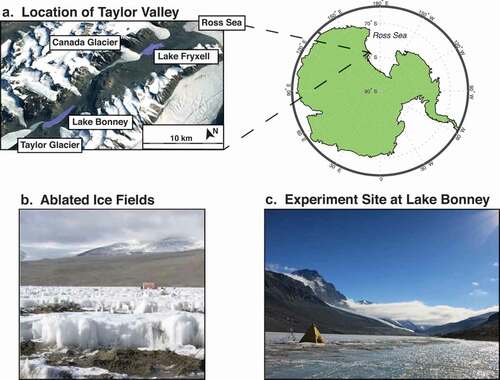
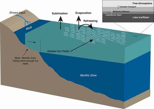
Although first-order relationships between wind regimes and latent heat flux can be readily inferred, the processes of lake–atmosphere exchange are more complicated than might be presumed from a perennially frozen surface. In the wintertime, the lake surfaces are entirely frozen under cold, dark conditions, and the latent flux is small and exclusively via sublimation. During the perpetually sunlit austral summer, moats (areas of liquid water that form along the lake edge) form, where evaporation exclusively occurs. The remaining frozen surface is mottled with pools of liquid water, some of which evaporates and some of which drains into the lake water underneath the ice via cracks or the moats or through channels in the surface ice. Some liquid water also refreezes on the lake surface (Figure 2). The strong winds and mixed-phase surface processes create DV lake surfaces that have rough topography with ice features that might rise a meter or more above the surface due to uneven areas of ablation and melting (Figures 1b, 1c). These ice features, along with dust accumulation and heterogenous snow distribution, contribute to localized ablation and melting via a positive feedback loop generated by additional surface wind shear and shadows (Dugan, Obryk, and Doran 2013).

Figure 2. Cross section of a dry valley lake as it would typically appear during the austral summer, depicting mechanisms of latent heat flux and possible isotopic fractionation type.

The heterogeneity of the surface relative to, for example, conditions on the accumulation zone of ice sheets makes it difficult to estimate total water losses from ablation stakes. Furthermore, direct hydrologic budgeting that might allow one to close the water balance is inhibited by uncertainty in subaqueous glacial melt volumes and the challenges of gauging small ephemeral streams. The use of eddy covariance as done by Clow et al. (1988)has been shown to be a useful approach to address this problem, but it has only been applied in limited circumstances.

Another approach to study long-term changes in the mass balance of lakes is to utilize stable isotope records (i.e., δ¹⁸O and δ²H) measured over time either directly from the lake reservoir or from paleorecords stored in carbonate sediments (Yapp 1979). If the stable isotopic ratio of the inputs (i.e., precipitation and stream flow) and outputs (latent heat flux) are known, then one can utilize a stable isotope mixing model to study changing hydrological budgets (Benson and Paillet 2002). This has been widely utilized to study the hydrological dynamics in tropical to boreal lake systems (e.g., Brooks et al. 2014; Gibson, Birks, and Yi 2016). Application of this approach to lake systems with perennial or seasonally extended ice cover, such as in the Dry Valleys, is difficult because the isotopic ratio of the latent heat flux from ice is challenging to estimate. Traditional efforts to estimate the isotopic ratio of the evaporative flux from lakes typically utilize the Craig-Gordon model (i.e., Craig and Gordon 1965) and take advantage of good constraints on the values for the isotopic fractionation during evaporation at temperatures greater than 0°C (Gibson, Edwards, and Prowse 1996; Gibson, Edwards, and Birks 1999). However, the degree of isotopic fractionation associated with sublimation remains a source of disagreement in the literature (Friedman, Benson, and Gleason 1991; Gustafson et al. 2010; Lécuyer et al. 2017). Furthermore, ablation is often a mixture of both sublimation and evaporation, so even if the fractionation factor associated with evaporation and sublimation were known, the relative mixture of the two would be difficult to estimate. Therefore, quantitative modeling of lake-level trends cannot fully take advantage of the stable isotope tracers unless an estimate of the isotopic fractionation associated with ablation can be reasonably constrained.

Here, we present measurements of the isotopic ratio of water vapor over Lake Bonney and Lake Fryxell during field campaigns in the summer of 2016–2017 and 2017–2018. We take advantage of a field deployable cavity ring-down spectrometer to make continuous isotopic measurements over the lake systems and use these data to generate an estimate of the isotopic ratio of the ablation flux. The goals of this analysis were to determine the magnitude of isotopic fractionation and the factors that control its variability, which is relevant to understanding how ablation impacts the isotopic ratio of the residual lake water and surface ice. Because of the short timescales of the campaigns presented here, we focus primarily on the drivers of diurnal and synoptic variations to generate first-order estimates of how changing wind speed, temperature, and relative humidity control the isotopic ratio of ablation.

Materials and methods

Site descriptions and equipment

Meteorological data

The experiments described here took place in front of Lake Bonney camp at the eastern side of the lake (77°36′24.22″ S, 162°26′59.56″ E) in November–December 2016 and in front of Lake Fryxell camp (77°36′24.22″ S, 163°7′30.31″ E) in January 2018. The experimental sites were selected based on where representative lake processes would occur while remaining within proximity to the camps’ power sources. At each location, a tripod was erected on the ice with a Vaisala HMP100 probe for temperature and relative humidity readings and an RM Young wind vane (model 05108) for wind velocity measurements, at heights of 3.0 and 0.5 m. An Apogee infrared radiometer was installed at 0.5-m height on the tripod to record lake surface skin temperatures. Air temperature, relative humidity, wind velocity, and lake surface temperature measurements were recorded every minute via a Campbell Scientific CR1000 data logger.

Ice and liquid water isotope data

Lake ice and water samples (from the surface water and at depth via SCUBA) were collected in vials, covered in parafilm, and transported to the laboratory for isotope analysis after the field campaign. Lake water samples were not collected at Lake Bonney due to lack of access to water, because it was early in the field season. At Lake Fryxell, surface water samples were collected within the moat and three water samples were collected underneath the ice cover at depths of 4.3, 5.5, and 6.4 m, near the experiment location where a hole had been drilled in the ice. Surface ice samples at both lakes were collected within 0 to 3 cm from the surface. Ice samples at Lake Bonney were collected daily near the tripod, and at Lake Fryxell samples were collected approximately twice per day under the tripod. Lake ice samples were also collected at Lake Fryxell along three transects spaced approximately every 300 to 500 m (meters) across the lake surface. The samples were processed via liquid injections into a Picarro A0211 vaporizer, connected to the same L2130-i analyzer deployed in the field (Gupta et al. 2009). In addition to presenting the individual hydrogen and oxygen isotope ratios, we present the deuterium excess, which is a useful indicator of kinetic fractionation associated with evaporation. Deuterium excess (d in the equation below) is calculated as (Dansgaard 1964; Clark and Fritz 1997)

(1) $d={\delta }^{2}H-8{\delta }^{18}O$(1)

Water vapor isotope flux measurements

Air inlets were installed at 0.5, 1.0, and 3.0 m on the tower using ¼″ OD Teflon tubes. The lines were insulated and continuously pumped at a flow rate of approximately 10 L min⁻¹ using a secondary pump. The lines were connected to a valve manifold that was programmed such that air at each height was sampled for 8-minute intervals; thus, data were recorded for all three heights over a 24-minute period before switching back to the first height to record the next 24-minute cycle. To remove memory effects between measurements at different heights, the data from the first 4 minutes of each 8-minute cycle were removed so that only the last half of each measurement interval was evaluated. The last 4 minutes of data did not contain any measurable trend and thus suggests that there was no remaining influence of measurements from the previous inlet (Supplemental Material S1). In addition, the inlet order and cycle were randomized to further minimize potential memory effects that might emerge from the persistent effect of measurement at one height onto another. This process was controlled through a custom air intake manifold that connects to the air inlet tubing and manages the air flow to the isotopic analyzer, in a design similar to that used by Berkelhammer et al. (2016). The analyzer was kept sheltered in a Scott tent on the lake ice surface or shoreline approximately 15 to 20 m from the tripod. The tubing between the tripod and the analyzer was placed on the lake ice surface and was covered and protected by foam casing to reduce the chance of it becoming embedded in the ice and ensuring that the air in the tube did not drop below the air temperature. Although we had atmospheric isotope data at three heights, we only utilize data from the 0.5- and 3.0-m heights to solve the flux gradient equations and ensure that the measurements were co-located with the heights of the meteorological data.

Isotope calibrations and adjustments

All vapor isotope data from the analyzer were first corrected for humidity effects (Bailey et al. 2015) and then normalized to Vienna Standard Mean Ocean Water (VSMOW; Gupta et al. 2009). The calibration and normalization were done by injecting liquid water standards into the Picarro A0211 vaporizer accessory for processing by the L2130-I analyzer. For atmospheric measurements, the humidity calibration was done in the lab at the DV camps, as well as outside in the Scott tent, by injecting a known standard into the vaporizer and adjusting the size of the injection and the dilution with dry air (Bailey et al. 2015). The effect of humidity on measurements of the isotope ratio of δ¹⁸O-a and δ²H-a only became evident, relative to the variance of the measurements, when the humidity was below 1,000 ppm, which did not occur during the Lake Fryxell campaign and only occurred very briefly during a föhn wind event at Lake Bonney. Lastly, we normalized the measurements to the VSMOW-Vienna Standard Light Antarctic Precipitation (VSLAP) scale by analyzing five reference standards during the field campaign (Coplen 1988). To account for instrument drift, different normalization equations were used for the Lake Bonney vs. Lake Fryxell campaigns, because both campaigns were conducted just over a year apart. The calibration procedures were completed in the lab prior to deployment, three times in the field during deployment, and again in the lab postdeployment.

Isotopic fractionation and δ_vapor calculations

The isotopic ratio of the ablating vapor flux (δ_vapor) was calculated using the gradient diffusion method as developed by Lee, Kim, and Smith (2007) and Xiao et al. (2017). The theory that underlies the gradient diffusion method is that the water vapor at any two heights contains a mixture of both a well-mixed background vapor and the vapor that is evaporating/sublimating from the surface. The presence of an isotopic gradient implies a different relative mixture of these two end-members (background and surface flux) in air mass following the rationale for the Keeling plot method to infer the isotopic ratio of a CO₂ source if the concentration and isotopic ratio of air masses at two heights are measured (Miller and Tans 2003). The gradient diffusion method is formally expressed as

(2) $R_{\mathrm{v}\mathrm{a}\mathrm{p}\mathrm{o}\mathrm{r}}=\frac{M_{O18,\mathrm{H}\mathrm{e}\mathrm{i}\mathrm{g}\mathrm{h}\mathrm{t}1}-M_{O18,\mathrm{H}\mathrm{e}\mathrm{i}\mathrm{g}\mathrm{h}\mathrm{t}2}}{q_{\mathrm{H}\mathrm{e}\mathrm{i}\mathrm{g}\mathrm{h}\mathrm{t}1}-q_{\mathrm{H}\mathrm{e}\mathrm{i}\mathrm{g}\mathrm{h}\mathrm{t}2}},$(2)

where M is the molar concentration of the isotopologue at each height (mol/L or ppm) and q is humidity (ppm). In this case, heights 1 and 2 represent the 0.5- and 3.0-m air inlets. The R_vapor ratio is then converted to δ_vapor (Clark and Fritz 1997):

(3) ${\delta }^x{Y}_{\mathrm{v}\mathrm{a}\mathrm{p}\mathrm{o}\mathrm{r},\mathrm{V}\mathrm{S}\mathrm{M}\mathrm{O}\mathrm{W}}=\left(\frac{R_{\mathrm{a}\mathrm{b}\mathrm{l}\mathrm{a}\mathrm{t}\mathrm{i}\mathrm{o}\mathrm{n}}}{R_{\mathrm{V}\mathrm{S}\mathrm{M}\mathrm{O}\mathrm{W}}}-1\right)\ast 1000.$(3)

This procedure can be done for both oxygen and hydrogen isotopes using R_VSMOW for ¹⁸O and deuterium. We predominantly discuss ¹⁸O, because deuterium and ¹⁸O strongly covary and thus the latter only provides redundant information (Results section). The gradient diffusion method is only applicable under the conditions of a fully turbulent atmospheric boundary layer. Because periods with a lack of turbulence (defined as a boundary layer with Richardson number greater than 0.19; see Latent Heat Flux Calculations section) lack a latent heat flux, they also must lack a latent heat flux for all isotopologues of water. Consequently, we do not report values when the latent heat flux values were less than 3 W/m².

In this study, we discuss isotopic fractionation associated with ablation using the enrichment factor, ε, which is related to the fractionation factor, α, using the following equation (Clark and Fritz 1997):

(4) ${\epsilon }_{\mathrm{I}\mathrm{c}\mathrm{e}/\mathrm{W}\mathrm{a}\mathrm{t}\mathrm{e}\mathrm{r}-\mathrm{V}\mathrm{a}\mathrm{p}\mathrm{o}\mathrm{r}}=\left(\frac{R_{\mathrm{I}\mathrm{c}\mathrm{e}/\mathrm{W}\mathrm{a}\mathrm{t}\mathrm{e}\mathrm{r}}}{R_{\mathrm{V}\mathrm{a}\mathrm{p}\mathrm{o}\mathrm{r}}}-1\right)\times {10}^3=\left({\alpha }_{\mathrm{I}\mathrm{c}\mathrm{e}/\mathrm{W}\mathrm{a}\mathrm{t}\mathrm{e}\mathrm{r}-\mathrm{V}\mathrm{a}\mathrm{p}\mathrm{o}\mathrm{r}}-1\right)\times {10}^3,$(4)

where R_ice/water is the ratio between heavy and light isotopes of the lake surface layer. The ε_{Ice/Water-Vapor} enrichment factor represents the apparent isotopic separation between the lake surface and the ablation flux leaving the surface. The magnitude of ε_{Ice/Water-Vapor} is the sum of equilibrium and kinetic fractionation associated with both the phase change and diffusion of vapor from the saturated surface layer to the free atmospheric boundary layer. High boundary layer turbulence tends to suppress kinetic fractionation by reducing the depth of the stable, thin saturated surface layer where diffusion drives fractionation. Low humidity is associated with higher kinetic fractionation because it reduces the degree of equilibration between the atmosphere and surface water reservoir (Gonfiantini et al. 2018).

Modeling of the isotopic ratio of ablation flux

We compare our measured δ_vapor fluxes to the most widely used model, the Craig-Gordon model (Craig and Gordon 1965), to compare how existing approaches to estimating this term perform. To estimate the value of the equilibrium fractionation factor, we use the equations of Majoube (1971):

(5) ${10}^{3}ln\left({\alpha }_{\mathrm{e}\mathrm{q}}^{18}{O}_{\mathrm{I}\mathrm{c}\mathrm{e}/\mathrm{W}\mathrm{a}\mathrm{t}\mathrm{e}\mathrm{r}-\mathrm{V}\mathrm{a}\mathrm{p}\mathrm{o}\mathrm{r}}\right)=1.137\left(\frac{{10}^6}{T^2}\right)-0.4156\left(\frac{{10}^3}{T}\right)-2.0667$(5)

(6) ${10}^{3}ln\left({\alpha }_{\mathrm{e}\mathrm{q}}^2{H}_{\mathrm{I}\mathrm{c}\mathrm{e}/\mathrm{W}\mathrm{a}\mathrm{t}\mathrm{e}\mathrm{r}-\mathrm{V}\mathrm{a}\mathrm{p}\mathrm{o}\mathrm{r}}\right)=24.844\left(\frac{{10}^6}{T^2}\right)-76.248\left(\frac{{10}^3}{T}\right)+52.612,$(6)

where T is temperature of the lake surface (measured by infrared radiometry) in Kelvin. These equations represent water–vapor phase change and can be assumed to be continuous across the 0°C line, because both Lake Fryxell and Lake Bonney exist as solid and liquid phase during austral summer. There are a number of various equilibrium fractionation equations available, and they are consistent with one another for temperatures above −20°C for α¹⁸O (Ellehoj et al. 2013). During these experiments, lake surface temperatures remained consistently above −20°C.

The kinetic fractionation factor (ε_k) will vary depending on turbulence and humidity conditions. Here, we estimate ε_k as

(7) ${\epsilon }_k=C_k\left(1-h\right),$(7)

where h is relative humidity and C_k = (D′/D)ⁿ − 1 (Gat 1996). D′/D is the diffusivity ratio of heavy to light isotopes and n is a turbulence parameter ranging from 0 (fully turbulent) to 1 (fully stable). We use the D′/D ratios determined by Cappa et al. (2003) with D(H₂¹⁸O)/D(H₂¹⁶O) = 0.9691 and D(HD¹⁶O)/D(H₂¹⁶O) = 0.9839. We use an n value of 0.5 to reflect intermediate conditions (mixture of turbulent and stable conditions as experienced during the field campaign; Leuenberger and Ranjan 2021). In general, ε_k values over lakes, especially frozen lakes, are not well constrained, because both humidity and boundary layer conditions can affect ε_k. Actual ε_k may be much lower or near zero during conditions of higher boundary layer turbulence as the complex topography of the frozen lake surface generates higher surface roughness and more vigorous mixing between the surface saturated layer and the boundary layer. Using the Craig-Gordon equation (Craig and Gordon 1965), we use ε_equilibrium and ε_kinetic from above to predict δ_vapor:

(8) ${\delta }_{\mathrm{v}\mathrm{a}\mathrm{p}\mathrm{o}\mathrm{r}}=\frac{{\alpha }_{\mathrm{e}\mathrm{q}}^{-1}{\delta }_L-h{\delta }_a-{\epsilon }_{\mathrm{e}\mathrm{q}}-\left(1-h\right){\epsilon }_k}{1-h+{10}^{-3}\left(1-h\right){\epsilon }_k},$(8)

where α_eq is the equilibrium fractionation factor from Equation (5)(5) ${10}^{3}ln\left({\alpha }_{\mathrm{e}\mathrm{q}}^{18}{O}_{\mathrm{I}\mathrm{c}\mathrm{e}/\mathrm{W}\mathrm{a}\mathrm{t}\mathrm{e}\mathrm{r}-\mathrm{V}\mathrm{a}\mathrm{p}\mathrm{o}\mathrm{r}}\right)=1.137\left(\frac{{10}^6}{T^2}\right)-0.4156\left(\frac{{10}^3}{T}\right)-2.0667$(5) or (6) depending on the isotope evaluated, δ_L is the isotope composition of the lake surface ice, δ_a is the isotope composition of the atmosphere, and h is relative humidity. Modeled estimates of ε_{ice/Water-Vapor} were calculated from δ_vapor using Equations (3) and (4).

Uncertainty of δ_vapor measurements

Given the series of computations that raw data undergo prior to reporting normalized isotope values, it is important to identify and estimate the total uncertainty that propagates through the calculations. For δ¹⁸O-a, the raw data of our Picarro L2130-I exhibited a standard error of 0.03 per mill (δ²H-a is 0.17 per mill). During the normalization correction, an additional maximum 0.04 per mill error existed based on the standard error of raw data during the normalization procedure, for a total of 0.05 per mill error propagation post normalization for a given data point. The use of a liquid standard in lieu of a vapor standard may also add a small degree of uncertainty. As such, because δ_vapor was calculated using two heights with two isotope values each, the possible total error in δ¹⁸O_vapor propagated to approximately 0.07 per mill (δ²H-a is 0.23 per mill). Deuterium excess uncertainty was 0.3 per mill, calculated from equations in Froehlich, Gibson, and Aggarwal (2002). Corrections were made for humidity, although because humidity during the field campaigns remained above 1,000 ppm, its impacts are negligible. It is relevant to note that the most important aspect of the calculation is the gradient rather than the absolute isotope value, so even if there was bias from the actual correction to VSMOW, it would have limited influence on the δ_vapor estimate. In addition, ultimately the error is presented in Figures 3c and 3d for ε_{Ice/Water-Vapor}, which is larger than the analytical uncertainty and is the most relevant because ε_{Ice/Water-Vapor} is the focus of this study.

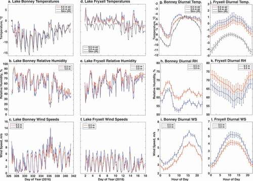
Figure 3. Meteorological data collected at both lakes. (a)–(f) Raw meteorological data (temperature, relative humidity, and wind speed) collected at Lake Bonney and Lake Fryxell during their respective field campaigns. (g)–(l) Mean hourly temperature, relative humidity, and wind speed on a typical day for both Lake Bonney and Lake Fryxell during their respective field campaigns, with standard error bars included.

Controls on the isotopic ratio of atmospheric water vapor

The δ¹⁸O-a is strongly controlled by the humidity (q) of the air under the dominant effect of Rayleigh distillation where drier air is isotopically more depleted. However, as Noone (2012) showed, the relationship between δ¹⁸O-a and q varies depending on the relative importance of mixing of air masses vs. distillation controls on the isotopic evolution of an air mass. Dynamics that affect δ¹⁸O-a vs. q spatially or temporally will affect the extent that changing ablation rates leave an isotopic impact on the residual water mass. The equation to evaluate water vapor fluxes under the Rayleigh distillation model is as follows:

(9) $\left(\delta -{\delta }_0\right)=\left({\alpha }_{eq}-1\right)\mathrm{l}\mathrm{n}\left(\frac{q}{q_0}\right),$(9)

where δ is the modeled isotope value (δ¹⁸O-a here), δ₀ is the isotope value of the source air mass, α_eq is the temperature-dependent equilibrium fractionation factor calculated from Equation (5)(5) ${10}^{3}ln\left({\alpha }_{\mathrm{e}\mathrm{q}}^{18}{O}_{\mathrm{I}\mathrm{c}\mathrm{e}/\mathrm{W}\mathrm{a}\mathrm{t}\mathrm{e}\mathrm{r}-\mathrm{V}\mathrm{a}\mathrm{p}\mathrm{o}\mathrm{r}}\right)=1.137\left(\frac{{10}^6}{T^2}\right)-0.4156\left(\frac{{10}^3}{T}\right)-2.0667$(5) , q is humidity (ppm), and q₀ is initial humidity of the source air mass. For a humid air mass originating in the McMurdo Sound/Ross Sea (at 0°C) that undergoes only Rayleigh distillation until it reaches the DV lakes region, we estimate a q₀ of 6,050 ppm (saturation humidity at 0°C and δ₀ of −11.3 per mill; Wei et al. 2019). This line assumes 100 percent precipitation efficiency, and lower values of humidity generally correlate to lower temperatures and therefore higher α_eq. In this model, temperature acts as an independent variable tied to humidity (q), such that saturation humidity levels decrease with decreasing temperature.

To model the effect of mixing between air masses with different δ¹⁸O-a and q values, we used the following equation from Noone (2012:)

(10) $\delta =q_{\mathrm{e}\mathrm{n}\mathrm{d}}\left({\delta }_{\mathrm{e}\mathrm{n}\mathrm{d}}-{\delta }_F\right)\frac{1}{q}+{\delta }_F.$(10)

δ_F represents the isotope flux of the mixing air source and q_end and δ_end represent the dry end-member humidity and δ¹⁸O-a composition, respectively. First, we model an ocean source with a δ_F (δ¹⁸O-a) of −11.3 per mill, which represents an approximation of the isotope composition of the air mass from the nearby ocean (Wei et al. 2019). Second, we model a land-based mixing scenario with δ_F (δ¹⁸O-a) of −35 per mill, an estimate of the air mass above the nearby ice sheet. We chose a value of −35 per mill, which is typical of values measured during austral summer (Wei et al. 2019). For both ocean source and land source mixing model scenarios, q_end and δ_end (the final values after the evolution of the air mass) are assumed to be 1,000 ppm and δ¹⁸O = −45 per mill, typical values of precipitation from very dry air masses on the Antarctic Ice Sheet during its coldest month, July (Noone 2008). The δ¹⁸O of −45 per mill used in our model is also in the range of observations taken by Wei et al. (2019). The q variable in Equation (10)(10) $\delta =q_{\mathrm{e}\mathrm{n}\mathrm{d}}\left({\delta }_{\mathrm{e}\mathrm{n}\mathrm{d}}-{\delta }_F\right)\frac{1}{q}+{\delta }_F.$(10) is an independent humidity variable input into the model for both the ocean source and land-based mixing scenarios. In situ q versus atmospheric δ¹⁸O data is compared to modeled trajectories of either rainout or mixing to provide insight into the regional water cycling in the DVs.

Latent heat flux calculations

To estimate the total water vapor and energy flux from the lakes, we used the two-level eddy correlation method employed by Box and Steffen (2001), which is based on the flux gradient method or K-theory (Thornthwaite and Holzman 1939). In this method, turbulence of mass, momentum, and heat is represented by the eddy diffusivities of the air (Munn 1966; Stull 1988). The two-level method latent heat flux, Q_L (W/m²), is calculated as

(11) $Q_L=-\rho L{u}_{\ast }^{2}K\left[\frac{\left(\frac{q_2-q_1}{z_2-z_1}\right)}{\left(\frac{u_2-u_1}{z_2-z_1}\right)}\right]{\mathrm{\Phi }}_E^{-1}{\mathrm{\Phi }}_M^{-1},$(11)

where ⍴ is air density (kg m⁻³), q is the specific humidity (kg kg⁻¹) at heights z₂ and z₁ (m), and u₂ and u₁ represent wind speed (m s⁻¹) at those heights as well. u_* represents friction velocity, and we follow the rationale from Box and Steffen (2001) in its calculation:

(12) $u_{\ast }=\frac{u_2{\left(\frac{z_2}{10}\right)}^{-1/7}}{26.5}.$(12)

Additionally, L represents the latent heats of sublimation (2.834 × 10⁶ J kg⁻¹) and evaporation (2.257 × 10⁶ J kg⁻¹), applied in the equation as appropriate.

For conditions of neutral turbulence, K represents the ratio of eddy diffusivities for momentum and water vapor (K_E/K_M) and the value is taken to be 1.35 (Stull 1988). Adjustments to the K term for nonneutral conditions are made through the stability correction functions (Φ_E Φ_M)⁻¹. This stability function term is equivalent to 1 for conditions of neutral turbulence, greater than 1 for conditions of greater than neutral turbulence, and less than 1 for conditions of less than neutral turbulence. A value of 0 represents a highly stable boundary layer condition where latent heat flux is not present (and thus Equation (11)(11) $Q_L=-\rho L{u}_{\ast }^{2}K\left[\frac{\left(\frac{q_2-q_1}{z_2-z_1}\right)}{\left(\frac{u_2-u_1}{z_2-z_1}\right)}\right]{\mathrm{\Phi }}_E^{-1}{\mathrm{\Phi }}_M^{-1},$(11) is equivalent to 0). Note that Equation (11)(11) $Q_L=-\rho L{u}_{\ast }^{2}K\left[\frac{\left(\frac{q_2-q_1}{z_2-z_1}\right)}{\left(\frac{u_2-u_1}{z_2-z_1}\right)}\right]{\mathrm{\Phi }}_E^{-1}{\mathrm{\Phi }}_M^{-1},$(11) contains a small correction in the exponent of the stability correction compared to Box and Steffen’s (2001) equation (3)(3) ${\delta }^x{Y}_{\mathrm{v}\mathrm{a}\mathrm{p}\mathrm{o}\mathrm{r},\mathrm{V}\mathrm{S}\mathrm{M}\mathrm{O}\mathrm{W}}=\left(\frac{R_{\mathrm{a}\mathrm{b}\mathrm{l}\mathrm{a}\mathrm{t}\mathrm{i}\mathrm{o}\mathrm{n}}}{R_{\mathrm{V}\mathrm{S}\mathrm{M}\mathrm{O}\mathrm{W}}}-1\right)\ast 1000.$(3) (Monteith and Unsworth 2013). The coefficients within the stability functions vary depending on whether stable, neutral, or turbulent conditions exist. The basic equation structures of these functions for both momentum and water vapor are

(13) $\mathrm{\Phi }={\left(1-\beta R_i\right)}^m$(13)

(14) $\mathrm{\Phi }={\left(1-\gamma R_i\right)}^n.$(14)

Equation (13)(13) $\mathrm{\Phi }={\left(1-\beta R_i\right)}^m$(13) represents conditions of greater than neutral turbulence, and Equation (14)(14) $\mathrm{\Phi }={\left(1-\gamma R_i\right)}^n.$(14) represents conditions of less than neutral turbulence. R_i represents the gradient Richardson number, and β, γ, m, and n are empirically derived parameters. These values vary in the literature, and we follow the convention of Steffen and DeMaria (1996) and Box and Steffen (2001) where β = 18, γ = 5.2, m = −1/4, and n = −1, because those studies were also conducted over an ice surface. In addition, Φ_E = Φ_M, except for more unstable conditions where R_i < −0.03. In this unstable case, Φ_E = (Φ_M/1.3). The dimensionless gradient Richardson number R_i is calculated as (Stull 1988)

(15) $R_i=\frac{g}{\stackrel{\prime }{{\theta }_v}}\frac{{\mathrm{\Delta }}_v}{\mathrm{\Delta }z}{\left(\frac{\mathrm{\Delta }\mathrm{u}}{\mathrm{\Delta }z}\right)}^{-2},$(15)

where g is gravitational acceleration of 9.81 m/s², $\stackrel{\prime }{{\theta }_v}$ is the average virtual potential temperature in Kelvin between heights 1 and 2, and Δθ_v is the virtual potential temperature difference between the two heights. Δz represents the distance (m), and Δu is the difference in wind speed (m/s) between the two heights. R_i values less than 0 represent unstable conditions. These negative R_i values then imply stability correction function (Φ_E Φ_M)⁻¹ values of greater than 1, thus correcting Q_L to more accurately reflect the higher latent heat flux expected during greater than neutral turbulence conditions. Similarly, R_i values of 0 represent neutral conditions and yield (Φ_E Φ_M)⁻¹ values of 1. R_i values greater than 0 represent less than neutral turbulence (mechanically driven turbulence) and yield (Φ_E Φ_M)⁻¹ values less than 1, thus correcting Q_L to accurately reflect the lower latent heat flux expected during these conditions. Given the value of γ = 5.2, the highest R_i value where any latent heat flux can occur is approximately 0.2 where (Φ_E Φ_M)⁻¹ approaches 0. Any R_i greater than 0.2 (also known as the critical Richardson number) is considered to represent a stable boundary layer where turbulent fluxes do not occur. The critical Richardson number is not universally agreed upon, but estimates range between 0.20 and 0.25 (Garratt 1992). As such, no latent heat flux (or δ_ablation) data are presented when R_i is greater 0.19, because assumptions in K theory then fail.

Results

Lake Bonney

Meteorological and lake surface temperature data

Air temperatures at both heights and on the lake surface were closely in phase with one another, though there was a gradient toward cooler temperature at the surface (Figure 3). The pattern was disrupted during the föhn wind event on day 336 when lake temperatures lagged the rapidly warming air and the lake temperature remained warm the day after the event, leading to a persistent period when the lake surface was warmer than the air. Over the course of the campaign, temperatures remained below freezing and showed a general warming trend except for the relatively warm conditions during the first two days of the campaign. Relative humidity normally fluctuated between 50 and 90 percent during the field campaign, except for the föhn event on day 336 where relative humidity dropped to near 30 percent. Wind speeds most often peaked around 5 to 6 m/s on a typical day, with the notable exception of the föhn wind event on day 336 where wind speeds exceeded 10 m/s. Diurnal cycles are evident for all meteorological measurements, with temperatures and wind speeds at highest levels midday, inversely proportional to relative humidity levels.

Isotopic composition of reservoirs

δ¹⁸O-i (lake ice composition) during the field campaign ranged between −38.3 and −35.4 per mill, with a mean composition of −37.1 per mill and a standard deviation of 1.24 per mill (Table 1). Lake ice did not show any long-term trends during the period of the campaign. However, a snow event did occur during the field campaign, and the snow had a mean δ¹⁸O of −33.5 per mill. Initial δ¹⁸O-i values during the field campaign of −38.2 per mill, however, were near the −37.8 per mill δ¹⁸O-i value of the final ice sampling on the final day of the field campaign. Thus, definitive changes in the isotopic composition of the lake surface ice were not detectable over the field campaign. Similarly, deuterium excess of lake ice at Lake Bonney is positive with values ranging between 16.0 and 22.4 per mill, with a mean value of 19.5 per mill and standard deviation of 1.8 per mill, consistent with previous studies that show Lake Bonney’s near surface waters have significantly higher deuterium excess values compared to the negative deuterium excess in the briny bottom waters (Gooseff et al. 2006). Consistent with δ¹⁸O-i data, no clear deuterium excess trend was observed over the campaign period. At Lake Bonney, the lake ice δ¹⁸O-i vs. δ²H-i regression slope is 7.06 (95 percent confidence interval [6.62, 7.51]), compared to 7.75 for McMurdo Dry Valley glaciers (Gooseff et al. 2006; Figure 4a). Slopes less than 8 are indicative of an evaporative regime with lower slopes indicative of more evaporative enrichment (Craig 1961). Lake water underneath the ice cover was not sampled during this campaign.

Table 1. Recent and historical isotopic measurements in Taylor Valley

Location	Recent measurement	Recent sample collection date/source	Previous measurement	Δ^18O, ‰ VSMOW (modern vs. historical samples)	Previous sample collection date/source
L. Fryxell surface ice δ^18O (‰ VSMOW)	−26.6 to −24.1	Jan. 2018, this study	−26.8 to −24.2	0.1 to 0.2	1987–1989, Miller and Aiken (1996)
			−27.3 to −25.0	0.7 to 0.9	Jan. 1972, Matsubaya et al. (1979)
L. Fryxell subsurface water δ^18O(‰ VSMOW)	−31.1 to −30.2	Jan. 2018, this study	−32.3 to −30.2	0 to 1.2	1987–1989, Miller and Aiken (1996)
			−31.8 to −30.4	0.2 to 0.7	Jan. 1972, Matsubaya et al. (1979)
L. Bonney surface ice (east lobe) δ^18O(‰ VSMOW)	−38.3 to −35.4	Nov–Dec. 2016, this study	N/A	N/A	N/A
L. Bonney subsurface water (east lobe) above chemocline δ^18O (‰ VSMOW)	−41.0 to −39.0	2002, Gooseff et al. (2006)	−42.4 to −38.3	−0.7 to 1.4	Jan. 1972, Matsubaya et al. (1979)
			−43.4 to −42.0	2.4 to 3.0	Dec. 1963, Hendy et al. (1977)
L. Fryxell ice deuterium excess	−9.1 to −3.0	Jan. 2018, this study (transect range)	−8.4 to −2.8	N/A	1988, calculated from Miller and Aiken (1996)
L. Bonney ice deuterium excess (east lobe)	16.0 to 22.4	Nov–Dec. 2016, this study (tower site)	N/A	N/A	Jan. 1972, shallow water (5 m) depths: 18.4 to 22.6 range, calculated from Matsubaya (1979)

Figure 4. Representations of current lake and atmospheric regression lines for (a) Lake Bonney and (b) Lake Fryxell. The Global Meteoric Water Line (GMWL) is in black, and individual atmospheric observations used to calculate the atmospheric regression lines are in gray.

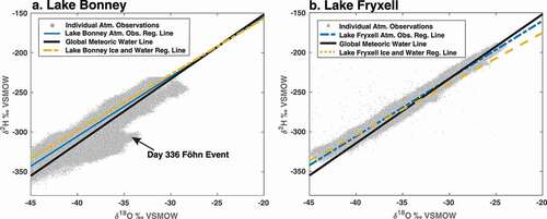
The δ¹⁸O-a (atmospheric vapor composition) over Lake Bonney varied between −48 and −31 per mill (Figure 5a). These values are consistent with those measured elsewhere in polar regions, including previous studies over the Antarctic and Greenland ice sheets (Steen-Larsen et al. 2013; Ritter et al. 2016). Although the Lake Bonney field campaign was too short to capture the seasonal cycle, the data do indicate a persistent diurnal cycle and evidence of significant synoptic variability in the isotopic ratio of the water vapor. These variations represent a combination of changing temperatures and source regions (i.e., upwind glacial vs. marine boundary layer air; Kurita et al. 2016). For example, a strong isotopic change associated with the onset of föhn winds on day 336 was observed. This event is observable as a clear deviation in the δ¹⁸O-a/δ²H space, as well as abnormally negative atmospheric deuterium excess values observed on this day, with values less than −30 per mill. These abnormally negative deuterium excess values are possible, because Lai and Ehleringer (2011)observed δ¹⁸O-a values of −40 per mill associated with periods of enhanced entrainment prior to storm events. The q vs. δ¹⁸O-a plots (Figure 6) suggest that atmospheric water vapor over Lake Bonney generally reflects air masses that are mixed with land/polar ice sheet based sources. The q vs. δ¹⁸O-a plots also demonstrate Lake Bonney’s generally low humidity and isotopically depleted boundary layer water vapor relative to Lake Fryxell. The Lake Bonney δ¹⁸O-a vs. δ²H-a regression slope value is 7.52 (95 percent confidence interval [7.515, 7.525]).

Figure 5. (a), (b) Normalized δ¹⁸O-a values at 0.5- and 3-m heights, as well as lake ice surface values, at Lake Bonney (LB) and Lake Fryxell (LF). Data presented are raw isotope data at each height normalized using equations available through Supplemental Material (S2). At Lake Bonney, there was a significant föhn wind event on day 336 and at Lake Fryxell, a small snow event on days 9 to 10. (c), (d) Red box and whisker plots showing calculated values of ε¹⁸O (ε_{Ice/Water-Vapor}) of the observed δ_ablation at Lake Bonney and Lake Fryxell, using Equations (2)(2) $R_{\mathrm{v}\mathrm{a}\mathrm{p}\mathrm{o}\mathrm{r}}=\frac{M_{O18,\mathrm{H}\mathrm{e}\mathrm{i}\mathrm{g}\mathrm{h}\mathrm{t}1}-M_{O18,\mathrm{H}\mathrm{e}\mathrm{i}\mathrm{g}\mathrm{h}\mathrm{t}2}}{q_{\mathrm{H}\mathrm{e}\mathrm{i}\mathrm{g}\mathrm{h}\mathrm{t}1}-q_{\mathrm{H}\mathrm{e}\mathrm{i}\mathrm{g}\mathrm{h}\mathrm{t}2}},$(2) –(6(6) ${10}^{3}ln\left({\alpha }_{\mathrm{e}\mathrm{q}}^2{H}_{\mathrm{I}\mathrm{c}\mathrm{e}/\mathrm{W}\mathrm{a}\mathrm{t}\mathrm{e}\mathrm{r}-\mathrm{V}\mathrm{a}\mathrm{p}\mathrm{o}\mathrm{r}}\right)=24.844\left(\frac{{10}^6}{T^2}\right)-76.248\left(\frac{{10}^3}{T}\right)+52.612,$(6) ). Red lines in the ε_{Ice/Water-Vapor} boxes are median values, and the top and bottom of the box represents the distribution between 75 and 25 percent of data points. For ε_Craig-Gordon boxes (black, offset), targets represent median values, and while the top and bottom of the box represents the distribution between 75 and 25 percent of modeled data points. (e), (f) Latent heat flux for Lake Bonney and Lake Fryxell, calculated for 100 percent sublimation and 100 percent evaporation end members, using Equations (10)–(14).

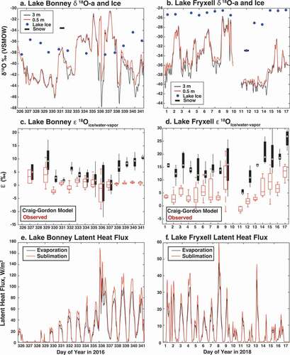
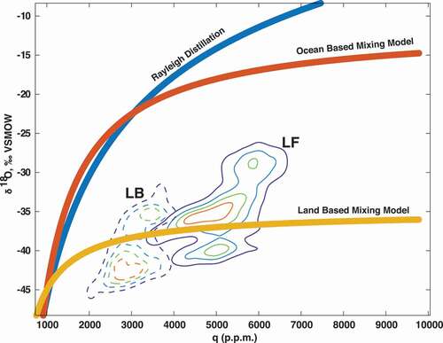
Figure 6. Analysis of boundary layer humidity (q) versus δ¹⁸O-a at Lake Bonney and Lake Fryxell for better constraining local water vapor sources. Dashed lines represent occurrence density contour lines at Lake Bonney, and solid lines represent occurrence density contour lines at Lake Fryxell. The thick blue line is the zone of predicted Rayleigh distillation, the red line represents a 100 percent ocean-based mixing model, and the yellow line represents a 100 percent land-based mixing model. Boundary layer vapor origins at both lakes suggest a primarily land-based origin.

ε_{Ice/Water-Vapor} Results

During the Lake Bonney campaign, ε_{Ice/Water-Vapor} remained consistently below the value that would be predicted under the Craig-Gordon model (Figure 3c). The calculated values of ε_{Ice/Water-Vapor} at Lake Bonney during the first few days of the experiment were generally higher compared to the remainder of the experiment. These higher values occurred during a period of low latent heat flux and higher boundary layer stability (Figure 3e). For the latter part of the campaign, the magnitude of boundary layer turbulence and associated latent heat flux were higher. During high latent heat flux periods, the ε_{Ice/Water-Vapor} values remained near or even below 0 per mill and did not approach that predicted by the Craig-Gordon model. However, day-to-day changes in ε_{Ice/Water-Vapor} at Lake Bonney did follow estimates from the Craig-Gordon model such that the model was correlated to observations but biased.

A snow event of at least 5 to 8 cm (from local community reports) occurred at Lake Bonney on day 331–332 which covered the lake with snow that was isotopically enriched in heavy isotopes relative to the lake ice (−33.4 per mill of snow compared to average lake ice δ¹⁸O of −37.1 per mill). Because our sample collection targeted the ice, the values of ε_{Ice/Water-Vapor} used for days 332 onward use the snow isotope composition as an estimate of the source δ¹⁸O-i for ablation used in Equation (4).

Latent heat flux

During the early portion of the experiment at Lake Bonney, there was very little latent heat flux but a significant diurnal cycle in latent heat flux emerged around day of year 331, with daytime peaks often exceeding 50 W/m². A significant föhn wind event occurred on day 336, when the latent heat flux reached values over 150 W/m². After day 336, latent heat flux remained elevated through the remainder of the experiment. Lake Bonney’s latent heat flux values generally fall within the same ranges observed during late spring on the Greenland ice sheet by Box and Steffen (2001). Based on the latent heat flux data, we estimate that Lake Bonney experienced mean ablation rates of approximately 0.91 mm/day in November–December 2016. For comparison, Clow et al. (1988) calculated ablation rates at Lake Hoare (located geographically between Lake Fryxell and Lake Bonney) and presented mean ablation rates between 0.82 and 1.61 mm/day in November and between 1.58 and 1.81 mm/day in January.

Lake Fryxell

Meteorological and lake surface temperature data

Air temperatures at Lake Fryxell often peaked above 0°C during the middle of the day, although generally air temperatures dropped below freezing in the evenings (Figure 3). Lake ice surface temperatures at the field site consistently remained below 0°C, but liquid water and moats were present during the period of the campaign, indicating that there were some areas of the lake with above-freezing surface temperatures. The lake surface temperatures were more decoupled from the air than at Lake Bonney, which may again reflect that the campaign was conducted later in the season and because of the thermal inertia of the thick ice layer, the surface is not likely to reach temperatures close to 0°C. Wind speeds exhibited consistent daily cycles between near-calm conditions to 6 to 7 m/s. Relative humidity values ranged between 40 and 85 percent, also varying diurnally and generally anti-phased with wind speed. The lower humidity values (~40 percent) were infrequent and occurred briefly during the daily wind speed maximum when drier air aloft was mixing to the lake surface. Diurnal cycles are evident for all meteorological measurements, with temperatures and wind speeds peaking midday, inversely proportional to relative humidity levels, as expected.

Isotopic ratios of reservoirs

The Lake Fryxell δ¹⁸O-w (lake water composition) at 4.3, 5.5, and 6.4 m was −30.2, −31.1, and −31.1 per mill, respectively. The δ²H-w of these three samples was −238.5, −243.0, and −242.9 per mill. Thirteen water samples were also taken from the liquid moat, and the mean δ¹⁸O-w value was −26.2 per mill, with a standard deviation of 0.3 per mill. Mean δ²H-w of moat water was −215.2 per mill with a standard deviation of 1.6 per mill.

δ¹⁸O-i during the field campaign ranged between −26.6 and −24.1 per mill, with a mean composition of −25.4 per mill and a standard deviation of 1.48 per mill, inclusive of the samples taken under the tower and those under the transects. Mean δ²H-i was −210.1 per mill with a standard deviation of 9.8 per mill. Individually, the ice under the tower had a mean δ¹⁸O-i of −25.6 per mill and a standard deviation of 2.3 per mill, with a mean δ²H-i of −211.6 per mill and standard deviation of 15.4 per mill. In the transects, mean δ¹⁸O-i was −25.3 per mill with a standard deviation of 0.7 per mill and a mean δ²H-i of −209.3 per mill with a standard deviation of 4.3 per mill (Figure 7). Thus, during the field campaign, variations in surface ice isotope compositions over the two-week field campaign at the tower site were greater than those exhibited geographically across the three transects. Overall temporal changes in the δ¹⁸O-i were not detectable over the period of the campaign. Deuterium excess of lake ice at Lake Fryxell was generally negative (as opposed to Bonney) with values ranging between −8.5 and 4.4 per mill, with a mean value of −6.5 per mill and standard deviation of 2.3 per mill. Consistent with δ¹⁸O-i data, no clear change in deuterium excess trend was observed (beginning value −8.4 per mill, end value −7.6 per mill), and the values did not vary systematically across transects (Figure 7). At Lake Fryxell, the lake ice and water δ¹⁸O-i/w vs. δ²H-i/w regression slope is 6.44 (95 percent confidence interval [6.27, 6.62]), suggesting that Lake Fryxell experiences significant evaporation.

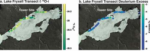
Figure 7. (a) Geographic distribution of δ¹⁸O-i in three transects at Lake Fryxell. (b) Geographic distribution of deuterium excess in three transects at Lake Fryxell.

The δ¹⁸O-a (atmospheric vapor composition) over Lake Fryxell varied approximately between −42 and −26 per mill (Figure 5b), similar to the range observed at Lake Bonney. The data indicate a persistent diurnal cycle and evidence of significant synoptic variability in the isotopic ratio of the water vapor. The q vs. δ¹⁸O-a plots (Figure 6) suggest that atmospheric water vapor over Lake Fryxell includes the presence of air masses that are mixed with land/polar ice sheet based sources. The q vs. δ¹⁸O-a plots also demonstrate the air over Lake Fryxell is generally more humid (compared to Lake Bonney). The Lake Fryxell δ¹⁸O-a vs. δ²H-a regression slope value is 7.28 (95 percent confidence interval [7.276, 7.28]). This is close to that of Lake Bonney and suggests that local effects on the lakes are small and that the systems are affected by the same air masses.

ε_{Ice/Water-Vapor} Results

During the Lake Fryxell campaign, ε_{Ice/Water-Vapor} also remained consistently below the value that would be predicted from the Craig-Gordon model (Figure 3d). Lake Fryxell’s ε_{Ice/Water-Vapor} values varied between ~0 and 12 per mill and appear to have experienced two cycles of ε_{Ice/Water-Vapor} fluctuations: the first from Julian days 1 to 9 in 2018 as ε_{Ice/Water-Vapor} approached a value comparable to predictions from the Craig-Gordon model on day 9 and the second in days 11 to 17 where ε_{Ice/Water-Vapor} exceeds model predictions on day 17. Some snowfall also occurred around day 10, though the snow event was light. The δ¹⁸O-s (snow isotope composition) that fell at Lake Fryxell on day 10 ranged between −32.8 and −32.9 per mill, and although this value is depleted in heavy isotopes compared to the snow-free ice surface, the impact of the snow event disappeared after a day. A clear diurnal cycle is observable at lake Fryxell, with ε_{Ice/Water-Vapor} values decreasing to lower levels during midday and then increasing to higher levels later in the day and overnight. Lake Fryxell’s ε_{Ice/Water-Vapor} values also were lower than that predicted by the Craig-Gordon model, yet day-to-day changes in ε_{Ice/Water-Vapor} mirrored those day-to-day changes predicted by the Craig-Gordon model fairly well, such that the model predictions were well correlated with observations yet biased (as with Bonney).

Latent heat flux

Lake Fryxell had much lower latent flux levels throughout the experiment duration relative to Lake Bonney. After the snow event on day 10, daily latent heat values remained low, with some days exhibiting maximum latent heat flux values less than 10 W/m². Overall, the latent heat flux values observed at Lake Fryxell were also within the bounds of −20 to 90 W/m² observed during late spring on the Greenland Ice sheet by Box and Steffen (2001). Based on the latent heat flux data, we estimate that Lake Fryxell ablated, on average, 0.28 mm/day in January 2018.

The latent heat flux–ε_{Ice/water-Vapor} relationship at both lakes

Higher latent heat fluxes (and thus higher boundary layer turbulence) tended to be associated with lower values of ε_{Ice/Water-Vapor} at both lakes (Figure 8d). Thus, the periods of highest mass loss were also the periods of the weakest isotopic enrichment of the residual ice. This relationship was true at both lakes during both field campaigns. Higher wind speeds and lower relative humidity contribute to higher latent flux at both lakes, and lower wind speed and higher relative humidity were associated with higher ε_{Ice/Water-Vapor} (Figures 8a, 8b). The diurnal cycle in latent flux (and boundary layer turbulence) is therefore not in phase with the ε_{Ice/Water-Vapor} daily cycle, because ε_{Ice/Water-Vapor} tended to increase throughout the day as boundary layer turbulence decreased. Low Richardson numbers (higher turbulence) are associated with daytime warming (Figure 8c) and precede the increase in ε_{Ice/Water-Vapor.} In addition, high latent heat flux days are associated with low ε_{Ice/Water-Vapor} during those days and vice versa. At Lake Fryxell, days 4, 8, and 13 had high latent heat flux, yet ε_{Ice/Water-Vapor} generally remained lower than lower latent heat flux days 3, 15, and 16.

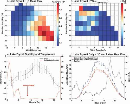
Figure 8. (a) Water vapor mass flux as a function of wind speed and relative humidity, with warmer colors expressing higher mass flux at both lakes. (b) ε¹⁸O (ε_{Ice/Water-Vapor}) as a function of wind speed and relative humidity at both lakes, with warmer colors representing higher ε¹⁸O. (c) Lake Fryxell hourly average Richardson number and hourly average 3 m temperature. Lower Richardson number denotes greater instability. (d) Mean hourly epsilon and latent heat flux values at Lake Fryxell during the experimental period.

Discussion

Since the 1960s, studies have utilized water isotope measurements in the Dry Valleys to understand first-order hydrological pathways and the legacy of rising and falling lake levels (Henderson et al. 1965; Hendy et al. 1977). However, these works have relied on minimal constraints on the isotopic fractionation associated with ablation. Notwithstanding the direct effects of runoff and recharge to changing lake levels, if ablation is strongly fractionating, then the shrinking of a lake would significantly enrich the residual lake mass even if the initial mass of the lake was not very large. On the other hand, if ablation is only minimally fractionating, then major reductions in lake levels would only have minor impacts on the isotopic ratio of the residual lake. We present the first comprehensive analysis of water vapor isotopes in the Dry Valleys with the intent of showing how lake–atmosphere exchange influences the isotopic ratio of the perennial ice cover. This ultimately influences the isotopic ratio of the sub-ice lake water (all lake water underneath under the ice cover) even though the signal is complicated by the additional fractionation associated with ice forming on to the bottom of the ice cover. This happens because surface melt can mix with sub-ice lake water through cracks in the ice as well as through moats, with the isotope impact affecting bottom waters via diffusion between isotope concentration gradients or other mixing dynamics depending on the lake. We estimated the magnitude of fractionation continuously during two multiweek periods in the summers of 2016–2017 and 2017–2018 over Lake Bonney and Lake Fryxell, respectively. The results showed evidence of strong variations in the isotopic fractionation associated with ablation over diurnal and synoptic timescales that can be used to make inferences on the factors, specifically boundary layer stability and humidity, that influence fractionation during ablation.

One of the primary results that emerged from these field campaigns was that during much of the experimental period at Bonney and during some of the time at Fryxell, ε_{Ice/Water-Vapor} values were not significantly different than 0 per mill. This result suggests that the combined kinetic and equilibrium effects yielded no fractionation during ablation. One interpretation of these low fractionation values is that sublimation was the predominant form of latent heat exchange and that sublimation from frozen lake surfaces does not fractionate water isotopes. The underlying justification for this, if true, would be that if ice sublimated directly from a solid crystal lattice structure to gas, it would not be possible to preferentially sublimate lighter isotopes because the diffusion rate in ice is too slow. Our observations contradict other work from alpine snowpack and polar firn that appear to have observed fractionation associated with sublimation (Cooper 1998; Hachikubo et al. 2000; Ritter et al. 2016). We hypothesize that other studies have demonstrated fractionation from sublimation because the observations were conducted on ice sheets or in laboratory experiments with porous surface layers (i.e., firn or snowpack). Under these conditions, vapor travels through the porous ice and fractionation occurs due to recondensation on colder surfaces, where isotopically heavier vapor preferentially condenses (Sokratov and Golubev 2009). These drivers of fractionation from sublimating ice systems would not be the case over a frozen lake where the water is sublimated directly from the surface layer without any tortuous pathway through a firn or snowpack. In addition, isotopic diffusion within snow may occur more rapidly than in ice (Lacelle et al. 2011). Here, during periods of turbulent mixing over the lake surface, kinetic fractionation is also limited due to the thinner saturated layer over the lake surface, where the residence time of water vapor is much less than the rate of diffusion of water vapor in air.

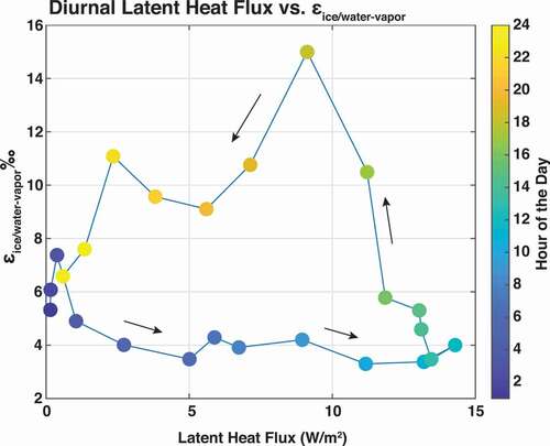
The data also show that though there were periods of nonfractionating ablation, there were other periods when ε_{Ice/Water-Vapor} reached values as high as 12 per mill. These periods of high fractionation (which were observed only over Lake Fryxell) indicate that the residual lake mass would become isotopically enriched through ablation, consistent with evaporating lake systems in nonpolar environments. Though we did not have sufficient data to study the seasonality or interannual variance of this process, the presence of diurnal and synoptic variability in both ε_{Ice/Water-Vapor} and latent heat flux over the campaign periods enable some insight into the relationship between the rate of ablation and the isotopic effect this has on the lake. At both Fryxell and Bonney, the latent heat flux had a diurnal pattern that peaks near noon, in phase with daily cycle of incoming radiation. On the contrary, ε_{Ice/Water-Vapor} exhibited a consistent minimum in the middle of the days and showed its peak values a few hours later when the boundary layer began to stabilize during earlier evening (Figure 8c). The high ε_{Ice/Water-Vapor} does not remain present through the stable nighttime period but rather drops to values close to zero and remains that way as radiation and latent heat flux rise again the next day. Therefore, ε_{Ice/Water-Vapor} did not respond in a monotonic way to latent heat flux nor temperature; rather, we hypothesize that the evening increase in ε_{Ice/Water-Vapor} reflects the gradual buildup of liquid water pools on the surface during the day that evaporate and lead to an isotopically fractionated latent heat flux. This pool is exhausted and ablation once again returns to be driven by sublimation with minimal fractionation. This out-of-phase cycle of latent heat flux and ε_{Ice/Water-Vapor} emerges as a well-characterized hysteresis loop (Figure 9a). We note that the pattern described above did not emerge at Bonney, which likely reflects that the data at this site were collected during an earlier and cooler period of the summer when temperature may not have exceeded a threshold to allow for the buildup of surface water pools. However, as we will discuss later, the conditions observed at Fryxell where the system transitioned between fractionating and nonfractionating ablation may rarely emerge at the generally cooler Bonney system.

Figure 9. (a) Overview of the mean latent heat flux vs. mean ε¹⁸O_{Ice/Water-Vapor}, by hour, on a daily timescale at Lake Fryxell. During periods of increasing latent heat flux in the first part of the day, ε¹⁸O_{Ice/Water-Vapor} remains low. As latent heat flux begins to decrease later in the day, ε¹⁸O_{Ice/Water-Vapor} begins to increase. Arrows signify direction of the cycle. (b) Overview of the cycle of mean latent heat flux vs. mean ε¹⁸O_{Ice/Water-Vapor} over days 3 to 9.

The daily cycle from low to high ε_{Ice/Water-Vapor} at Lake Fryxell was also overlain by a pair of multiday cycles of low to high ε_{Ice/Water-Vapor} fluctuations. During the experiment, this synoptic scale cycle occurred on days 1 to 9 and again on days 11 to 17. As with the diurnal cycle, we hypothesize that this cycle represents the buildup of liquid water pools following warm and stable days that become exhausted over a multiday period as high turbulent conditions emerge. These periodic events reset the system, as observed by ε_{Ice/Water-Vapor} dropping quickly back to values near 0 per mill around day 9. Though the experimental period only allowed us to capture two of these cycles, they likely represent the development and dissipation of larger scale pressure systems in the region and the associated effects on the temperature, wind conditions, and atmospheric stability profiles. The Craig-Gordon model partially reproduced these observed cycles, because the model effectively captured the influence of humidity associated with meteorological fluctuations. So, though the model was sufficiently sensitive to changing meteorology, the predicted values overestimated observed values of fractionation by not accounting for the nonfractionating process of sublimation. We see that daily boundary layer turbulence is related to surface temperatures, and weather patterns may affect surface temperatures and turbulence conditions (Figure 8c). For example, at Lake Fryxell, multiday cycles of relative humidity fluctuations observed during the field campaign could have been a control on ε_{Ice/Water-Vapor} fluctuations because such relative humidity cycles appear in addition to the diurnal cycle. Local maxima of relative humidity during the field campaign, which are associated with latent heat flux minima, correspond to higher values of ε_{Ice/Water-Vapor.} Though the direct proportionality of relative humidity and ε_{Ice/Water-Vapor} may seem counterintuitive due to the impact of humidity on kinetic fractionation, it suggests that boundary layer stability levels contribute more to ε_{Ice/Water-Vapor} than relative humidity levels alone in this system.

The negative relationship between latent heat flux and ε_{Ice/Water-Vapor} that emerges at Fryxell on both diurnal and synoptic scales also is reflected in the differences between the data collected at Bonney vs. Fryxell. This is, the early season campaign at Bonney was associated with high latent heat flux but low ε_{Ice/Water-Vapor}, whereas the opposite was true at Fryxell. We cannot confirm that the conditions observed during these short campaigns were necessarily representative of persistent differences between the Bonney and Fryxell systems. However, because the differences between lakes and from different periods of the year mirror the diurnal and synoptic patterns, we believe this is a generalized condition where latent heat flux and the magnitude of fractionation are inversely related. The clearest manifestation of this effect was during the föhn wind event at Bonney when the conditions were optimal for high rates of ablation but with apparently no isotopic enrichment of the underlying ice. Similarly, at Lake Fryxell, the time of day with the highest latent heat flux was associated with the lowest ε_{Ice/Water-Vapor}; thus, isotopic enrichment of the ice was very limited. Ice surface temperatures at Lake Fryxell peaked near freezing during the height of daytime radiative flux; therefore, some surface melting may have occurred as the boundary layer stabilized, leading to evaporation and higher ε_{Ice/Water-Vapor} values. During periods when lake surface temperatures remain well below freezing, such as the conditions observed at Lake Bonney, this surface melting could not occur, and ablation effectively would not isotopically enrich the lake ice. This was seen at Lake Fryxell on days 12 to 13 when ice surface temperatures were the lowest during the field campaign and ε_{Ice/Water-Vapor} approached 0 per mill. Although these periods of higher ε_{Ice/Water-Vapor} occurred at Lake Fryxell, any significant shifts in the ice cover isotope composition over the field campaign were not detected. It is possible that any pools of water that formed evaporated entirely rather than refroze, or our sampling depth of up to 3 cm may have erased this signal.

The results presented here highlight the challenges to applying stable isotope mass balance approaches to DV or other icy lakes. If we consider how sensitive ε_{Ice/Water-Vapor} of the Fryxell system was to changing atmospheric conditions, it is easy to imagine how this value could vary significantly between years, or even between seasons. Changes in humidity and boundary layer stability alone can affect the type of ablation and the degree of fractionation and thus, changes in surface ice isotope composition at seasonal to multi-annual scales (Leng and Anderson 2003). Lake Fryxell, where δ¹⁸O-a was more enriched and experienced higher humidity conditions during its field campaign compared to that of Lake Bonney as seen in the q vs. δ¹⁸O-a plots, had lower latent heat flux, which limits the degree of lake enrichment, yet higher δ¹⁸O-a could imprint onto the lake ice by affecting the rate of diffusive fractionation through the saturated boundary layer. Because Lake Bonney and Lake Fryxell both plot along a similar trendline on the q vs. δ¹⁸O-a plots, it is reasonable to propose that conditions at Lake Bonney could approach that observed at Lake Fryxell during the field campaign at the height of summer in January or February or during a particularly warm year. Yet, differences in the hydraulic residence times between lakes, the more rapid warming of shallower lakes, and the overall cooler conditions at Lake Bonney may also play a role in ablation flux and its isotopic fractionation (Foreman, Wolf, and Priscu 2004; Kopec et al. 2018). Longer term isotope study in this region would help clarify how ε_{Ice/Water-Vapor,} and therefore ice surface isotope composition, changes at seasonal to longer scales.

Values of ε_{Ice/Water-Vapor} were not accurately predicted using the widely used Craig-Gordon model at either lake during their respective field campaigns; however, day-to-day changes in ε_{Ice/Water-Vapor} were predicted by the model. The observed values of ε_{Ice/Water-Vapor} could be achieved via the model only if fractionation factors reflecting the nonfractionation of sublimation were assumed. In such a scenario, sublimation would not leave an enriched signature on the isotope composition of the ice surface. Day-to-day increases or decreases in observed values of ε_{Ice/Water-Vapor} were in phase with day-to-day increases predicted by the model, suggesting that changes in physical observations of humidity and background atmosphere isotope composition translated to similar day-to-day changes in predicted isotope composition of the vapor flux. As such, this may signify that fractionation during sublimation of snowpack may be due recondensation on the surface within pore spaces within the snowpack rather than sublimation itself as other studies have proposed.

Despite the apparent sensitivity of ε_{Ice/Water-Vapor} and its highly nonlinear response to forcing, there is also evidence from our data that the variability and range of ε_{Ice/Water-Vapor} for the two lakes may be somewhat stable. We see from the surface transects from Lake Fryxell that δ¹⁸O-i is consistent across the large areas of the lake where measurements were taken, despite variations in ice smoothness from different ablation intensities, sand/dust content on the lake surface, and variations in depth along the transects. In addition, the lack of significant isotope composition change over the field campaign suggests that either the intensity of evaporation that occurred was not enough to leave an isotopic imprint on the surface or any water that melted evaporated entirely (especially at Lake Fryxell). In addition, lake ice thickness is at a steady state, and as ice ablates, new ice freezes on the bottom of the ice layer at the same rate of removal, which may also contribute to the stability of the isotope composition of the lake ice cover. Therefore, daily fluctuations in ε_{Ice/Water-Vapor} do not lead to similar daily fluctuations in the isotope composition of the lake ice.

The topographic and climatological differences between the locations of the two lakes may generate conditions unique to each lake. Lake Fryxell’s lower δ¹⁸O-i vs. δ²H-i regression slope compared to Lake Bonney also suggests that the higher ε_{Ice/Water-Vapor} observed at Lake Fryxell than at Lake Bonney may be typical. Thus, Lake Bonney may experience less evaporation in favor of sublimation, and Lake Fryxell experiences more evaporation. In addition, the negative deuterium excess observed in the surface ice at Lake Fryxell is indicative of the occurrence of evaporation. Lake Bonney’s surface ice had positive deuterium excess, which is anomalous relative to the deuterium excess values of stream and glacial inputs observed by Gooseff et al. (2006) but could occur as a result of partially evaporated precipitation inputs during very dry conditions or from a groundwater source (Mikucki et al. 2015). If significant evaporation had occurred at Lake Bonney prior to the field campaign, we would expect lower deuterium excess results. This may be largely due to geographic and topographic differences between the two lakes. Lake Fryxell is located in an open area of Taylor Valley, closer to the Ross Sea, with more direct and constant sunlight, encouraging more ice melt in austral summer. Lake Bonney is located within a steeper region of Taylor Valley where mountains can obscure direct sunlight from parts of the day, limiting ice melt. In addition, Lake Bonney is located nearer to the East Antarctic Ice Sheet and can experience föhn winds more often, which can provide a mechanism for greater sublimation. Therefore, some of the observations during the field campaign may reflect these important topographic and climatological differences between the two lakes.

Though we focus primarily on measurements from these two recent field campaigns, there is a wealth of information on the isotopic ratio of Dry Valley reservoirs that dates back for decades. These data have been utilized along with other tracers to provide critical constraints on the lakes’ histories (Hendy et al. 1977). As the observations reported here illustrated, estimating long-term trends or variability in ε_{Ice/Water-Vapor} would be challenging given that traditional models for estimating δ_vapor do not work well and that ε_{Ice/Water-Vapor} is affected by boundary layer stability, which is difficult to estimate from available meteorological records. As with Lake Fryxell, for example, we can see disparate modes of isotopic fractionation, and between years the system could deviate between one mode to another depending on the synoptic conditions during that year. Additional studies, conducted over seasonal or multi-annual time periods, would be critical for developing models that could be deployed in service of estimating long-term changes in the isotopic composition of Dry Valley lakes. Such studies could also help further constrain the hydrologic budget of the lakes and provide further insight on what contributions changes in ablation could have on rising lake levels.

Conclusions

Water isotopes in arctic and alpine lakes have been used to reconstruct lake-level histories, but these studies have relied on limited observations of δ_vapor. Here we explored how variations in ablation/latent heat flux impart a signal on the residual lake ice using in situ measurements of the isotopic ratio of the water vapor flux from the lakes. During the experimental periods in 2016–2017 and 2017–2018 at Lake Bonney and Lake Fryxell, higher values of the enrichment factor ε_{Ice/Water-Vapor} were associated with lower latent heat/water vapor flux from the lake surface. This was due predominantly to boundary layer dynamics in an energy-limited system, regulating isotope fractionation effects during ablation of the lake surface. The periods of highest ablation were those associated with dry winds and low humidity when lower values of ε_{Ice/Water-Vapor} were predominant. In addition, we found that sublimation of the lake ice surface is nonisotopically fractionating and that when comparing our results to the Craig-Gordon model, the model fails unless the equilibrium fractionation factor in the model is assumed to be zero. Longer term studies could provide important additional constraints on the hydrologic budgets of DV lakes, because long-term shifts in the isotopic composition of the lakes could signify changes in long-term ablation and therefore atmospheric boundary layer trends in the region. Better understanding of these processes may also provide further insight on larger questions such as the evolution of DV lake systems over long time periods, as well as other polar ice systems, and how the sediment record reflects past ice/atmosphere dynamics of arctic lakes or even the history of Mars’ ice caps.

Data availablity statement

Data archiving is currently underway and is planned to be stored at the McMurdo Dry Valleys LTER website data repository (www.mcm.lternet.edu). In the meantime, data is available publicly at: https://uofi.box.com/s/6vakvltbsn1nhrpzudffclrn5iufpoux.

Disclosure statement

No potential conflict of interest was reported by the authors.

Supplementary material

Supplemental material for this article can be accessed on the publisher’s website.

Additional information

Funding

This work was supported by the National Science Foundation/McMurdo (LTER C-511).

References

- Bailey, A., D. Noone, M. Berkelhammer, H. C. Steen-Larsen, and P. Sato. 2015. The stability and calibration of water vapor isotope ratio measurements during long-term deployments. Atmospheric Measurement Techniques 8 (10):4521–38. doi:https://doi.org/10.5194/amt-8-4521-2015.
- Benson, L., and F. Paillet. 2002. HIBAL: A hydrologic-isotopic-balance model for application to paleolake systems. Quaternary Science Reviews 21 (12–13):1521–39. doi:https://doi.org/10.1016/S0277-3791(01)00094-4.
- Berkelhammer, M., D. C. Noone, H. C. Steen-Larsen, A. Bailey, C. J. Cox, M. S. O’Neill, D. Schneider, K. Steffen, and J. W. C. White. 2016. Surface-atmosphere decoupling limits accumulation at Summit, Greenland. Science Advances 2:e1501704. doi:https://doi.org/10.1126/sciadv.1501704.
- Bomblies, A., D. M. McKnight, and E. D. Andrews. 2001. Retrospective simulation of lake-level rise in Lake Bonney based on recent 21-yr record: Indication of recent climate change in the McMurdo Dry Valleys, Antarctica. Journal of Paleolimnology 25:477–492. doi:https://doi.org/10.1023/A:101113141926.
- Box, J. E., and K. Steffen. 2001. Sublimation on the Greenland Ice sheet from automated weather station observations. Journal of Geophysical Research: Atmospheres 106 (D24):33965–81. doi:https://doi.org/10.1029/2001JD900219.
- Brooks, J., J. Gibson, S. Briks, M. Weber, K. Rodecap, and J. Stoddard. 2014. Stable isotope estimates of evaporation: Inflow and water residence time for lakes across the United States as a tool for national lake water quality assessments. Limnology and Oceanography 59 (6):2150–65. doi:https://doi.org/10.4319/lo.2014.59.6.2150.
- Cappa, C., M. Hendricks, D. DePaolo, and R. Cohen. 2003. Isotopic fractionation of water during evaporation. Journal of Geophysical Research Atmospheres 108 (D16):4525. doi:https://doi.org/10.1029/2003JD003597.
- Clark, I., and P. Fritz. 1997. Environmental isotopes in hydrogeology. Boca Raton: Lewis Publishers.
- Clow, G. D., C. P. McKay, G. M. Simmons Jr., and R. A. Wharton Jr. 1988. Climatological observations and predicted sublimation rates at Lake Hoare, Antarctica. Journal of Climate 1:715–28. doi:https://doi.org/10.1175/1520-0442(1988)001<0715:COAPSR>2.0.CO;2.
- Cooper, L. 1998. Isotopic fractionation in snow cover. In Isotope Tracers in Catchment Hydrology, eds. C. Kendall and J.J. McDonnell, 119–36. Amsterdam: Elsevier.
- Coplen, T. B. 1988. Normalization of oxygen and hydrogen isotope data. Chemical Geology (Isotope Geoscience Section) 72:293–97. doi:https://doi.org/10.1016/0168-9622(88)90042-5.
- Craig, H., and L. I. Gordon. 1965. Deuterium and oxygen 18 variations in the ocean and the marine atmosphere. In Stable isotopes in oceanographic studies and paleotemperatures, ed. E. Tongiorgi, 9–130. Pisa: Consiglio Nazionale Delle Ricerche Laboratorio di Geologia Nucleare. n.d.
- Craig, H. 1961. Isotopic variations in meteoric waters. Science New Series 133 (3465):1702–03. May 26. doi:https://doi.org/10.1126/science.133.3465.1702.
- Dansgaard, W. 1964. Stable isotopes in precipitation. Tellus 16:436–68. doi:https://doi.org/10.1111/j.2153-3490.1964.tb00181.x.
- Doran, P. T., C. P. McKay, A. G. Fountain, T. Nylen, D. M. McKnight, C. Jaros, and J. E. Barrett. 2008. Hydrologic response to extreme warm and cold summers in the McMurdo Dry Valleys, East Antarctica. Antarctic Science 20:499–509. doi:https://doi.org/10.1017/S0954102008001272.
- Dugan, H. A., M. K. Obryk, and P. T. Doran. 2013. Lake ice ablation rates from permanently ice-covered Antarctic lakes. Journal of Glaciology 59:491–98. doi:https://doi.org/10.3189/2013JoG12J080.
- Ellehoj, M. D., H. C. Steen-Larsen, S. J. Johnsen, and M. B. Madsen. 2013. Lake-ablation equilibrium fractionation factor of hydrogen and oxygen isotopes: Experimental investigations and implications for stable water isotope studies: Lake-ablation equilibrium fractionation factor. Rapid Communications in Mass Spectrometry 27:2149–58. doi:https://doi.org/10.1002/rcm.6668.
- Foreman, C., C. Wolf, and J. Priscu. 2004. Impact of episodic warming events on the physical, chemical, and biological relationships of lakes in the McMurdo Dry Valleys, Antarctica. Aquatic Geochemistry 10:239–68. doi:https://doi.org/10.1007/s10498-004-2261-3.
- Fountain, A., G. Saba, B. Adams, P. Doran, W. Fraser, M. Gooseff, M. Obryk, J. Priscu, S. Stammerjohn, and R. Virginia. 2016. The impact of a large-scale climate event on Antarctic ecosystem processes. BioScience 66 (10):848–63. doi:https://doi.org/10.1093/biosci/biw110.
- Friedman, I., C. Benson, and J. Gleason. 1991. Isotopic changes during snow metamorphism. In Stable isotope geochemistry: A tribute to Samuel Epstein, 211–21. San Antonio: Geochemical Society.
- Froehlich, K., J. Gibson, and P. Aggarwal. 2002. Deuterium excess in precipitation and its climatological significance. Study of environmental change using isotope techniques. C&S Papers Series 13/P, 54–65. Vienna, Austria: International Atomic Energy Agency.
- Garratt, J. R. 1992. The atmospheric boundary layer, Cambridge atmospheric and space science series. Cambridge; New York: Cambridge University Press.
- Gat, J. 1996. Oxygen and hydrogen isotopes in the hydrologic cycle. Annual Review of Earth and Planetary Sciences 24:225–62. doi:https://doi.org/10.1146/annurev.earth.24.1.225.
- Gibson, J., S. Birks, and Y. Yi. 2016. Stable isotope mass balance of lakes: A contemporary perspective. Quaternary Science Reviews 131 (Part B):316–28. doi:https://doi.org/10.1016/j.quascirev.2015.04.013.
- Gibson, J., T. Edwards, and S. Birks. 1999. Pan-derived isotopic composition of atmospheric water vapor and its variability in northern Canada. Journal of Hydrology 217 (1–2):55–74. doi:https://doi.org/10.1016/S0022-1694(99)00015-3.
- Gibson, J., T. Edwards, and T. Prowse. 1996. Development and validation of an isotopic method for estimating lake evaporation. Hydrological Processes 10:1369–82. doi:https://doi.org/10.1002/(SICI)1099-1085(199610)10:10<1369::AID-HYP467>3.0.CO;2-J.
- Gonfiantini, R., L. I. Wassenaar, L. Araguas-Araguas, and P. K. Aggarwal. 2018. A unified Craig-Gordon isotope model of stable hydrogen and oxygen isotope fractionation during fresh or saltwater evaporation. Geochimica et Cosmochimica Acta 235:224–36. doi:https://doi.org/10.1016/j.gca.2018.05.020.
- Gooseff, M. N., J. E. Barrett, B. J. Adams, P. T. Doran, A. G. Fountain, W. B. Lyons, D. M. McKnight, J. C. Priscu, E. R. Sokol, C. Takacs-Vesbach, et al. 2017. Decadal ecosystem response to an anomalous melt season in a polar desert in Antarctica. Nature Ecology & Evolution 1:1334–38. doi:https://doi.org/10.1038/s41559-017-0253-0.
- Gooseff, M. N., W. B. Lyons, D. M. McKnight, B. H. Vaughn, A. G. Fountain, and C. Dowling. 2006. A stable isotopic investigation of a polar desert hydrologic system, McMurdo Dry Valleys, Antarctica. Arctic, Antarctic, and Alpine Research 38:60–71. doi:https://doi.org/10.1657/1523-0430(2006)038[0060:ASIIOA]2.0.CO;2.
- Gupta, P., D. Noone, J. Galewsky, C. Sweeney, and B. H. Vaughn. 2009. Demonstration of high‐precision continuous measurements of water vapor isotopologues in laboratory and remote field deployments using wavelength‐scanned cavity ring‐down spectroscopy (WS‐CRDS) technology. Rapid Communications in Mass Spectrometry 23:2534–42. doi:https://doi.org/10.1002/rcm.4100.
- Gustafson, J., P. Brooks, N. Molotch, and W. Veatch. 2010. Estimating snow sublimation using natural chemical and isotopic tracers across a gradient of solar radiation. Water Resources Research 46:W12511. doi:https://doi.org/10.1029/2009WR009060.
- Hachikubo, A., S. Hashimoto, M. Nakawo, and K. Nishimura. 2000. Isotopic mass fractionation of snow due to depth hoar formation. Polar Meteorology and Glaciology 14:1–7.
- Henderson, R. A., W. M. Prebble, R. A. Hoare, K. B. Popplewell, D. A. House, and A. T. Wilson. 1965. An ablation rate for Lake Fryxell, Victoria Land, Antarctica. Journal of Glaciology 6:129–33. doi:https://doi.org/10.1017/S0022143000019110.
- Hendy, C. H., A. T. Wilson, K. B. Popplewell, and D. A. House. 1977. Dating of geochemical events in Lake Bonney, Antarctica, and their relation to glacial and climate changes. New Zealand Journal of Geology and Geophysics 20:1103–22. doi:https://doi.org/10.1080/00288306.1977.10420698.
- Kopec, B., X. Feng, E. Posmentier, J. Chipman, and R. Virginia. 2018. Use of principal component analysis to extract environmental information from lake water isotopic compositions. Limnology and Oceanography 63:1340–54. doi:https://doi.org/10.1002/lno.10776.
- Kurita, N., N. Hirasawa, S. Koga, J. Matsushita, H. C. Steen-Larsen, V. Masson-Delmotte, and Y. Fujiyoshi. 2016. Influence of large-scale atmospheric circulation on marine air intrusion toward the East Antarctic coast: Marine air intrusion to the Antarctica. Geophysical Research Letters 43:9298–305. doi:https://doi.org/10.1002/2016GL070246.
- Lacelle, D., M. Fontaine, A. Forest, and S. Kokelj. 2011. High-resolution stable water isotopes as tracers of thaw unconformities in permafrost: A case study from western Arctic Canada. Chemical Geology 368:85–96. doi:https://doi.org/10.1016/j.chemgeo.2014.01.005.
- Lai, C., and J. Ehleringer. 2011. Deuterium excess reveals diurnal sources of water vapor in forest air. Oecologia 165:213–23. doi:https://doi.org/10.1007/s00442-010-1721-2.
- Lécuyer, C., A. Royer, F. Fourel, M. Seris, L. Simon, and F. Robert. 2017. D/H fractionation during the sublimation of water ice. Icarus 285:1–7. doi:https://doi.org/10.1016/j.icarus.2016.12.015.
- Lee, X., K. Kim, and R. Smith. 2007. Temporal variations of the 18O/16O signal of the whole-canopy transpiration in a temperate forest: Isotopic signal of canopy transpiration. Global Biogeochemical Cycles 21:n/a–n/a. doi:https://doi.org/10.1029/2006GB002871.
- Leng, M., and N. Anderson. 2003. Isotopic variation in modern lake waters from western Greenland. The Holocene 13 (4):605–11. doi:https://doi.org/10.1191/0959683603hl620rr.
- Leuenberger, M. C., and S. Ranjan. 2021. Disentangle kinetic from equilibrium fractionation using primary (δ17O, δ18O, δD) and secondary (Δ17O, dex) stable isotope parameters on samples from the Swiss precipitation network. Frontiers in Earth Science 9:Article 5980681. March. doi:https://doi.org/10.3389/feart.2021.598061.
- Majoube, M. 1971. Oxygen-18 and deuterium fractionation between water and water vapor. Journal de Chimie Physique et de Physiochimie Biologique 68:1423. doi:https://doi.org/10.1051/jcp/1971681423.
- Matsubaya, O., H. Sakai, T. Torii, H. Burton, and K. Kerry. 1979. Antarctic saline lakes—stable isotopic ratios, chemical compositions and evolution. Geochimica et Cosmochimica Acta 43:7–25. doi:https://doi.org/10.1016/0016-7037(79)90042-5.
- Mikucki, J., E. Auken, S. Tulaczyk, R. Virginia, C. Schamper, K. Sorensen, P. Doran, H. Dugan, and N. Foley. 2015. Deep groundwater and potential subsurface habitats beneath an Antarctic dry valley. Nature Communications 6:6831. doi:https://doi.org/10.1038/ncomms7831.
- Miller, J., and P. Tans. 2003. Calculating isotopic fractionation from atmospheric measurements at various scales. Tellus B: Chemical and Physical Meteorology 55 (2):207–14. doi:https://doi.org/10.3402/tellusb.v55i2.16697.
- Miller, L. G., and G. R. Aiken. 1996. Effects of glacial meltwater inflows and moat freezing on mixing in an ice-covered antarctic lake as interpreted from stable isotope and tritium distributions. Limnology and Oceanography 41:966–976. doi:https://doi.org/10.4319/lo.1996.41.5.0966.
- Monteith, J. L., and M. H. Unsworth. 2013. Principles of environmental physics. 4th ed. Oxford: Academic Press, Inc.
- Munn, R. E. 1966. Descriptive micrometeorology. Oxford: Academic Press, Inc.
- Noone, D. 2008. The influence of midlatitude and tropical overturning circulation on the isotopic composition of atmospheric water vapor and Antarctic precipitation. Journal of Geophysical Research 113:D04102. doi:https://doi.org/10.1029/2007JD008892.
- Noone, D. 2012. Pairing measurements of the water vapor isotope ratio with humidity to deduce atmospheric moistening and dehydration in the tropical midtroposphere. Journal of Climate 25:4476–94. doi:https://doi.org/10.1175/JCLI-D-11-00582.1.
- Ritter, F., H. C. Steen-Larsen, M. Werner, V. Masson-Delmotte, A. Orsi, M. Behrens, G. Birnbaum, J. Freitag, C. Risi, and S. Kipfstuhl. 2016. Isotopic exchange on the diurnal scale between near-surface snow and lower atmospheric water vapor at Kohnen station, East Antarctica. The Cryosphere 10:1647–63. doi:https://doi.org/10.5194/tc-10-1647-2016.
- Sokratov, S. A., and V. N. Golubev. 2009. Snow isotopic content change by sublimation. Journal of Glaciology 55:823–28. doi:https://doi.org/10.3189/002214309790152456.
- Steen-Larsen, H. C., S. J. Johnsen, V. Masson-Delmotte, B. Stenni, C. Risi, H. Sodemann, D. Balslev-Clausen, T. Blunier, D. Dahl-Jensen, M. D. Ellehøj, et al. 2013. Continuous monitoring of summer surface water vapor isotopic composition above the Greenland Ice Sheet. Atmospheric Chemistry and Physics 13 (9):4815–28. doi:https://doi.org/10.5194/acp-13-4815-2013.
- Steffen, K., and T. DeMaria. 1996. Surface energy fluxes of Arctic winter sea ice in Barrow Strait. Journal of Applied Meteorology 35:2067–79. doi:https://doi.org/10.1175/1520-0450(1996)035<2067:SEFOAW>2.0.CO;2.
- Stull, R. B. 1988. An introduction to boundary layer meteorology. Dordrecht: Kluwer Academic Publishers.
- Thornthwaite, C., and B. Holzman. 1939. The determination of evaporation from land and water surfaces. Monthly Weather Review 67:4–11. doi:https://doi.org/10.1175/1520-0493(1939)67<4:TDOEFL>2.0.CO;2.
- Wei, Z., X. Lee, F. Aemisegger, M. Benetti, M. Berkelhammer, M. Casado, K. Caylor, E. Christner, C. Dyroff, O. García, et al. 2019. A global database of water vapor isotopes measured with high temporal resolution infrared laser spectroscopy. Scientific Data 6 (1):180302. doi:https://doi.org/10.1038/sdata.2018.302.
- Xiao, W., X. Lee, Y. Hu, S. Liu, W. Wang, X. Wen, M. Werner, and C. Xie. 2017. An experimental investigation of kinetic fractionation of open-water evaporation over a large lake: Kinetic effect of lake evaporation. Journal of Geophysical Research: Atmospheres 122 (21):11,651–11,663. doi:https://doi.org/10.1002/2017JD026774.
- Yapp, C. J. 1979. Oxygen and carbon isotope measurements of land snail shell carbonate. Geochimica et Cosmochimica Acta 43:629–35. doi:https://doi.org/10.1016/0016-7037(79)90170-4.