Mass balance of two perennial snowfields: Niwot Ridge, Colorado, and the Ulaan Taiga, Mongolia

ABSTRACT

Perennial snowfields are generally receding worldwide, though the precise mechanisms causing recessions are not always well understood. Here we apply a numerical snowpack model to identify the leading factors controlling the mass balance of two perennial snowfields that have significant human interest: Arapaho Glacier, located at Niwot Ridge in the Colorado Rocky Mountains (United States), and a snowfield located in the Ulaan Taiga (Mongolia). The two locations were chosen because they differ in elevation, slope, and aspect. However, both have subarctic climates and are located within semi-arid regions. We show that for these two locations the snowfield mass balance is primarily sensitive to air temperature and wind speed, followed by precipitation and dust deposition amounts. The lack of sensitivity to dust deposition was most likely due to timing of deposition and the overall small dust amounts. We find that the sensitivities are similar for the center of the snowfield as well as the margins.

KEYWORDS:

• Arapaho Glacier
• Colorado
• Mongolia
• perennial snowfield
• perennial snowfield mass balance

Introduction and background

Perennial snowfields and glaciers have generally been receding or disappearing worldwide (e.g., Lemke et al. 2007; Vuille et al. 2008; Haugen et al. 2010; Rangwala and Miller 2012; Veettil and Kamp 2019). The presumed cause is that the global average temperature has increased by about 1.2°C from 1900 to the present (Hawkins et al. 2017; Sherwood et al. 2020). However, changes in wind speeds and snow accumulation (Fassnacht et al. 2018; Mott et al. 2018), as well as darkening due to snow algae (Dove et al. 2012), dust, and soot (Painter et al. 2007, 2013; Dozier et al. 2009; Gleason, Nolin, and Roth 2013; Skiles and Painter 2017, 2019), are also important processes, albeit more difficult to document.

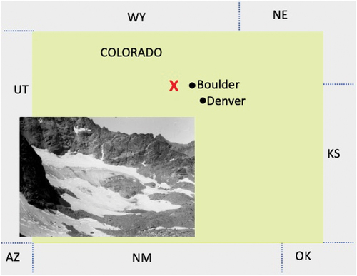
Our work is motivated by the following questions: Under what meteorological conditions will the perennial snowfields vanish, and what condition is most important? To address these questions, we evaluate the meteorological and physical conditions impacting the longevity of perennial snowfields in two specific locations: Arapaho Glacier, which is situated west of Boulder, Colorado, in the Colorado Rocky Mountains, and a perennial snowfield in the Ulaan Taiga mountains of northern Mongolia within a large area of tundra and larch forest. We chose these two specific locations because they represent two distinct classes of snowpacks. Arapaho Glacier is in a high-elevation mountainous region and the snowfields in the Ulaan Taiga mountains are at a lower elevation on comparatively flatter terrain.

In addition, both are of significant human interest. Mongolian perennial snowpacks serve as an important summer area for reindeer pastoralism (Taylor et al. 2019), and their loss would have cultural impact. The Arapaho Glacier is part of the Boulder Creek watershed, an important water source for Boulder, Colorado (Murphy 2006). The Arapaho Glacier is not flowing and is thus a perennial snowfield. Because of its use as a water source, there is a detailed record of the size of the Arapaho Glacier. Finally, the environmental data needed to operate our model are available for both sites.

Snowfield properties

Perennial snowfields, defined as snowfields that persist for at least an entire year, are a common feature of high-elevation landscapes (e.g., Higuchi et al. 1980; Fountain, Glenn, and Basagic 2017). They are distinguished from glaciers in two important ways. First, perennial snowfields do not flow; hence, mass accumulation and mass loss occur over the same area. Because they do not flow, the deepest layers of a snowfield date back to its origin. The second difference is that some perennial snowfields are present at elevations considerably lower than the elevations of glaciers. Dohrenwend (1984) showed that in the Western United States the lowest elevation at which perennial snowfields survived was 740 m lower than the glacial equilibrium line altitude. Thus, mountain ranges that completely lack glaciers may have perennial snowfields; for example, the Japanese Alps and all other mountain ranges in Japan (Higuchi et al. 1980).

Perennial snowfields are also found in very cold locations that have too little precipitation for glaciers. The lower elevations of the McMurdo Dry Valleys of Antarctica have numerous mountain glaciers (Fountain et al. 1998). At higher elevations snow input is greatly reduced (Fountain et al. 2010) and glaciers are replaced by perennial snowfields. For example, University Valley (77.86° S, 163.75° E, elevation 1,700 m), a hanging valley with a mean annual air temperature of −23.4°C (Goordial et al. 2016), does not have a glacier but has a large perennial snowfield at one end and several smaller perennial snowfields co-located with shallow ice-cemented ground on the valley floor (McKay 2009).

Because perennial snowfields can occur at relatively low elevations, they are often an important source of meltwater and cool conditions in summer (e.g., Garwood et al. 2020). Taylor et al. (2019) reported on perennial snowfields in Mongolia used in the summer by reindeer (Rangifur tarandus) pastoralists to cool heat-stressed animals. They found that in recent years, many of these features have begun to melt entirely for the first time in collective memory.

Snowfields can leave distinctive geological features known as “nivation hollows” due to increased mechanical particle transport and chemical weathering (Thorn 1976; Caine 1995). Eyles and Daurio (2015) reported on relict nivation hollows in Ubehebe Crater in Death Valley, California, whiched they suggest formed from snowfields during the recent Little Ice Age cooling, c. ~700 years B.P.

Perennial snowfields are also of archeological significance because they preserve organic material, ash deposits, and human artifacts associated with their use over thousands of years. Ødegård et al. (2017) and Pilo et al. (2021) reported on perennial snowfields in Norway for which the bottom ice is 7,600 and 6,900 years old, respectively.

Mechanisms impacting snowfield longevity

The persistence of a snowfield depends on snowfall amount, snow redistribution due to winds, avalanches, and ablation via sublimation and meltwater runoff. Fujita et al. (2010) reported on over forty years of ablation data at the Hamaguri‐yuki snowfield in the northern Japanese Alps and compared solar radiation, wind speeds, and air temperatures to meteorological records at the snowfield over five years and at a permanent weather-recording station 100 km from the snowfield. They concluded that the snowfield reduced the wind speed by modifying topography and thereby reduced ablation. They suggested that this positive feedback could stabilize snowfields. Mott et al. (2011) investigated these effects and concluded that snow surfaces in a depression—such as a nivation hollow—had reduced turbulent mixing compared to a flat snow surface. Mott et al. (2013) conducted field studies using local eddy flux measurements over snowfields and concluded that ablation was primarily dependent on wind velocity, turbulent intensity, fetch distance, and topographical curvature. Burns et al. (2014) conducted a similar study in seasonal snow on Niwot Ridge, Colorado, and reached similar conclusions, though their study was in a subalpine forest. There is, not surprisingly, a similarity between mechanisms that control the mass loss from a seasonal snowfield and a perennial snowfield. Perennial snowfields, however, are likely to have the added benefit of being nestled in hollows, cirques, or other natural wind shelters that not only decrease ablation but also drastically increase the snow input, through either drifting or snow cornice avalanching (Hansen, Chronic, and Matelock 1978).

Snow ablation can occur in two forms: sublimation and melt. There is evidence that sublimation can be responsible for the majority of ablation for glaciers in high altitudes and arid locations (Gascoin et al. 2013; Batbaatar et al. 2018). However, both the Ulaan Taiga and Arapaho Glacier are in regions with cold continental climates, with semi-arid conditions. Similar snowfields have sublimation losses of 10 to 30 percent of total seasonal ablation (Batbaatar et al. 2018; Sexstone et al. 2018; Stigter et al. 2018). Snowmelt initiation within the snowfield does not immediately result in complete snowfield ablation but instead initiates a complex process of snowfield ripening, refreezing of percolated water within the snow layers, and the eventual ablation of the snowfield via runoff and sublimation (DeWalle and Rango 2008), although sublimation losses occur prior to snowmelt as well. Dust may play a role in melt and sublimation by reducing the surface albedo of the snowfield. Other physical attributes such as snowpack elevation, slope, and aspect are fundamental controls on snowpack accumulation and ablation (Elder, Dozier, and Michaelsen 1991; Broberg 2021).

Characteristics of Arapaho Glacier and its environment

Arapaho Glacier, elevation ~3,680 m.a.s.l., is a complex glacial relic that has been studied for the past century (Waldrop 1964; Haugen et al. [2010] and references therein). Portions of Arapaho Glacier consist of ice (with a distinct bergschrund), together with other areas of coarse granular firn, overlain by seasonal snow. Arapaho Glacier has been receding since its historic stade maximum around 1860 (Waldrop 1964). In addition, since recordkeeping began in 1900, Waldrop (1964) found that Arapaho Glacier had thinned about 32 m. Since 1964, however, the glacier thinning has slowed, and Haugen et al. (2010) estimated it lost an additional 4.5 m between 1960 and 2005.

Arapaho Glacier (Figure 1) is situated in an eastward-facing cirque, with varying slope (Waldrop 1964). From Haugen et al. (2010) we estimate the steepest bed angle to be approximately 25° with a due east aspect. Elevation profiles in Haugen et al. (2010) indicate that the surface of the snowfield is not level with the bed surface. Photos indicate a steepened section of the snow surface in places; hence, we added another 5° to the slope of the surface for a total surface angle of 30°.

Figure 1. Arapaho Glacier, taken 27 August 1960. Site map of the Arapaho Glacier in Colorado, indicated by the red X, coordinates 40°01′24″ N 105°38′53″ W, elevation 3,680 m. The distance across the snowfield is about 600 m. The D1 site is also located at the red X, being less than 1 km from the glacier, and is therefore not shown at this scale. Neighboring states of Utah (UT), Wyoming (WY), Nebraska (NE), Arizona (AZ), New Mexico (NM), Oklahoma (OK), and Kansas (KS) are indicated. Image credit: Henry Waldrop, 1960. Arapaho Glacier: From the Glacier Photograph Collection. Boulder, Colorado: National Snow and Ice Data Center. Digital media. Source: http://nsidc.org/data/glacier_photo/search/image_info/arapaho_waldrop_084.

It is important to determine whether a snowfield is sliding, because we use that as our operational definition of a glacier (sliding) versus a perennial snowfield (not sliding). We approach this question in the manner of Fountain, Glenn, and Basagic (2017). Using the criterion of Fountain, Glenn, and Basagic (2017) for a perennial snowfield, we find that the computed basal shear stress for Arapaho Glacier is

(1)

where ρ is the ice density (using an upper limit of 900 kg m³), g is acceleration due to gravity (9.8 m/s²), h is thickness (m), and α is the surface slope angle.

Fountain, Glenn, and Basagic (2017) estimated h to be 15 m, so the basal shear stress b = 0.56 × 10⁵ Pa. The theoretical yield stress threshold of ice is 10⁵ Pa (Paterson 1994). Note that conservative values were chosen in order to obtain an upper limit to the basal shear stress. Given that the threshold yield stress of ice is greater than our calculated value of , Arapaho Glacier should not be moving, so it is classified here as a perennial snowfield rather than a glacier.

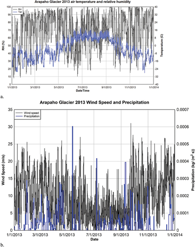
Meteorological conditions near Arapaho Glacier are available from an hourly Long-term Ecological Research (LTER) data set (Jennings and Molotch 2019) for the Niwot Ridge, Colorado, “D1” site, an alpine tundra site that has a similar elevation to Arapaho Glacier. The data set includes air temperature, relative humidity, wind speed, precipitation, downwelling shortwave (SW), and downwelling longwave (LW) for the period 1 January 2013 to 31 December 2013. The annual temperature and relative humidity are shown in Figure 2a for 2013. The annual average air temperature was −2.9°C and relative humidity was 68.9 percent for Arapaho Glacier. For June, July, and August, the average air temperature was 6.8°C and relative humidity was 63.2 percent. Wind speeds and precipitation are highly variable but much lower in summer than in winter, as shown in Figure 2b.

Figure 2. (a) Hourly measurements of air temperature (°C) and relative humidity (RH, %) for the Niwot Ridge data set, used to drive the Arapaho Glacier perennial snowfield model. T_air is the air temperature. (b) Wind speed and precipitation rate.

Characteristics of the Ulaan Taiga Mountains of Mongolia and their environment

The Ulaan Taiga Mountains have been experiencing a loss of glaciers and perennial snowfields within the last several decades (Taylor et al. 2019). Glacier area has decreased by ~30 percent over the last seventy years (United Nations 2018). Simulations with the ECHAM General Circulation Model predict snow cover decreases of ~33 percent by 2040 (United Nations n.d.).

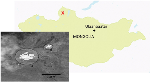
The elevation of the Mongolia snowfield in Figure 3 is 2,243 m. The slope for the Mongolian snowfield is close to 0°; photos from Taylor et al. (2019) indicate that at least one of the perennial snowfields was situated on an alluvial plain (Figure 3). Taylor et al. identified several approximate locations of receding perennial snowfields. The likely position of one of their identified sites, “Site 3,” is shown in the insert of Figure 3.

Figure 3. Site map of the perennial snowfields in Mongolia, coordinates 51°10′45″ N 98°58′06″ E, elevation 2,243 m. The red X marks the general location of the snowfields from Taylor et al. (2019). Insert A shows a snowfield that appears to be a river icing and a smaller snowfield (B) that appears to be on the shore of the stream. These snowfields are close to, perhaps identical to, Site 3 from Taylor et al. (2019). North is upward in the insert. Digital Globe Image was taken on 15 July 2015 and provided to the National Aeronautics and Space Admininstration with no restrictions on use or copying.

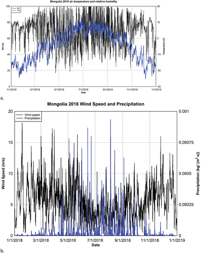
Atmospheric data sets for Mongolian snowfields are not available from local measurements. However, there are data from the MERRA-2 reanalysis data set (Gelaro et al. 2017). We use data for 2018. The location used for the meteorology data was a 0.625 × 0.5° grid cell centered on the point 52° N by 99° E. The output fields included date, local time, air temperature at 2 m height, specific humidity, downwelling SW, downwelling LW, wind at 2 m height, precipitation mass, and surface pressure. The air temperature and relative humidity are shown in Figure 4a. The annual average air temperature was −6.6°C, and the average relative humidity was 69.4 percent. For June, July, and August the average air temperature was 7.6°C and relative humidity was 66.0 percent. Hence, the ablation season air temperature was approximately 1°C warmer than Arapaho Glacier, and relative humidity was approximately 3 percent higher than Arapaho Glacier. Wind speeds were lower in summer than winter, but precipitation was greater in the summer.

Figure 4. (a) Hourly measurements of air temperature (°C) and relative humidity (%) used to drive the Ulaan Taiga perennial snowfield model. T_air is the air temperature. (b) Wind speed and precipitation rate.

Snowpack model

Description

The snowfield model used in this work is based on the model in K. E. Williams et al. (2008) and Heldmann et al. (2012). We use our model, instead of another popular model such as SNOWPACK (Lehning et al. 1999), because our model has a radiative transfer component that permits the detailed modeling of dusty snow. On the other hand, SNOWPACK does not explicitly model radiative transfer but instead uses an empirical scheme to model albedo decay based on meteorological conditions. SNOWPACK does not explicitly take dust and other albedo-reducing impurities into account.

Briefly, our model uses a finite volume approach that tracks energy and mass within a one-dimensional column of snow of variable depth underlain by 4 m of soil substrate. Layer thicknesses are kept at approximately 1 cm thick, though they are allowed to grow and shrink as the model evolves in time. If a given layer gets significantly thinner or thicker, we subtract a computational layer or add one. There is no maximum to the number of snow layers, though we have rarely run the model for more than 10 m of snow. The model is run until the sole remaining computational snow layer is less than 1 cm thick, at which point the snow is declared completely ablated.

The model uses a two-stream radiative transfer calculation (Toon et al. 1989; McKay et al. 1994) to find the energy deposition at depth for sunlight within the dusty snow column. The radiative transfer code includes scattering of light by dust and ice grains. The simplest way to include scattering in the visible part of the spectrum is through the use of a radiative transfer approach that considers separately radiation propagating downward and radiation propagating upward. These are known as “two-stream methods.” We use a variant of the two-stream method known as the “hemispheric constant,” in which all diffuse radiation moving in the upward direction is treated as a single upwelling irradiance term F⁻ and, similarly, for the downward diffuse radiation F⁺ (Meador and Weaver 1980). The direct solar beam is treated independently of the diffuse radiation. Further details and error analysis of the two-stream method is provided in Toon et al. (1989). The dust was assumed to be red Saharan dust, with 2-μm particle radii; the spectral albedo and asymmetry parameters were derived from measurements of the complex refractive index as reported in Patterson (1977). The optical properties for ice (snow) are from Warren (1984).

At the bottom of the 4 m soil substrate, the model uses an initial condition of the mean annual soil surface temperature and thereafter uses a bottom boundary condition of the geothermal heat flux. The upper boundary condition, at the snow surface, consists of a surface energy budget calculation. The surface energy budget terms include the sensible heat turbulent flux, latent heat turbulent flux, heat conduction out of the substrate, incoming solar shortwave, outgoing solar as determined from the snowpack albedo via the radiative transfer calculation, incoming longwave, and outgoing longwave. The sublimation is calculated via the latent heat flux, as given in Appendix 1, and depends principally on wind, temperature, and water vapor density. The equations used are discussed in K. E. Williams et al. (2008). Appendix 1 has additional details concerning the atmospheric turbulent flux calculations employed in the model.

The ablation rate and timing of loss of snow for our model were tested by comparison with both an empirical data set and model output from another popular and verified model: SNOWPACK (Lehning et al. 1999). We found that, for a seasonal snowpack, our meltout dates differed by less than one day from both the model and the observations. Appendix 3 has model validation details.

The model can be driven by either meteorological reanalysis output fields or observations at hourly intervals. We drive the model with fields that include date, time, air temperature, relative humidity, wind speed, downwelling SW flux, downwelling LW flux, and precipitation amounts. The sensible and latent heat turbulent fluxes are calculated, because the driving data sets do not provide these values. For the Ulaan Taiga region of Mongolia we used reanalysis output fields for 2018 from the MERRA-2 data set, and for Arapaho Glacier we used observations from 2013 (Jennings and Molotch 2019). We used 2013 for Arapaho Glacier because it was the most recent year for which data were available in the hourly LTER data set, and 2018 was used for Mongolia because the MERRA data set was likely to be well validated (Reichle et al. 2017; Baba et al. 2018).

Physical setting

Perennial snowfields may appear on flat ground as well as slopes. They are frequently located in cirques or on the lee side of ridges and often underneath wintertime snow cornices. Pomeroy et al. (2001) found that mean accumulation of snow water equivalent (SWE) on the lee side of a crest can be twice that of the windward slope and that snow cornices can contain six times the snow of the windward slope. Arapaho Glacier is primarily nourished by drifting snow, not direct precipitation (Hansen, Chronic, and Matelock 1978). According to our driving data set for the Niwot Ridge D1 station in 2013, snowfall ended by 31 May and began again on 22 September. For the Mongolia site in 2018, snow ended on 30 May and began on 4 September. In our model we simulate drifting snow by the daily deposition of clean snow, at midnight, on the simulated perennial snowfield surface for the months of snow deposition, using a temporally constant deposition amount. We discuss some limitations of our snow input model in the Discussion and Conclusion section in this text. The blowing snow does not occur continuously, but we have no independent blowing snow data that we can use to validate more discrete approaches. Using a simple threshold wind speed for blowing snow would be much too crude, given that the snow erodibility is not constant throughout the annual season. Note that the snowdrift deposit was in addition to episodic deposition in precipitation events via rain or snow. If rain occurs on top of the snow, the model determines via the existing layer mass and latent heat addition whether the existing snow mass and thermodynamics warrant melting of the snow and/or refreezing of the rain.

Images in Taylor et al. (2019), Haugen et al. (2010), and Waldrop (1964) indicate that perennial snowfields often have arcuate shapes with thinning edges. In the case of Arapaho Glacier, ground-penetrating radar surveys indicate that the edges are thin (but variable), with increasing depth near the center of the snowfield (Haugen et al. 2010). Arapaho Glacier is estimated to have a maximum thickness of 15 m (Haugen et al. 2010). The annual mass balance of the snowfield is therefore a function of the longevity of the thinner snow at the edges; if the edges are losing mass, then the center is most likely also losing mass. In addition, thin snow deposits may respond slightly differently to climate forcing than thicker snowfields, given that when snowfields get thinner than a few decimeters, the albedo of the substrate becomes relevant (Wiscombe and Warren 1980).

We therefore model perennial snowfields by focusing on the edges and, in particular, two initial thicknesses of 1.0 and 4.5 m for both Arapaho Glacier and the modeled perennial snowfield in the Ulaan Taiga. The thicknesses are set on 1 January; hence, they represent an initial depth of the snow column prior to any subsequent precipitation and ablation. An identical snowfield depth for both geographic locations was chosen to facilitate comparison. We chose to model depths of 1.0 m and 4.5 m for several reasons. First, thin 1-m snowfields were found in our modeling to be ephemeral, often disappearing by June. Such thin snowfields on the edge of the perennial snowfields may indicate sensitivities that thicker snowfields do not. Second, we found by experimentation that thicker 4.5-m snowfields were necessary because (a) they were able to survive an entire melt season until snow drifting began and (b) 4.5 m was thick enough so that only small daily amounts of snowdrift from September to May were needed to maintain an annual mass balance of zero over the single year being studied. The 1.0-m cases use the same drift as the 4.5-m cases (even though those amounts of wind drift will not lead a 1.0-m snowfield to have zero mass balance or, indeed, to survive for an entire year), in order to facilitate comparison.

Note that our 1-m cases are most likely not applicable to seasonal snowpacks, given that the modeled 1-m cases were assumed to be in the same geophysical setting as the 4.5-m cases (e.g., cirques or nivation hollows), and hence were subjected to the same intense snow input amounts that result in the 4.5-m cases having zero mass balance.

In general, mass balance is defined as

(2)

We analyze, in the Experiments section below, the sensitivity of the annual mass balance to constant air temperature warming, nighttime-only air temperature warming, wind speed, surface dust deposition amounts, and precipitation amounts. To study the effects of snowfield aspect, inclination, and position relative to adjacent surfaces on annual mass balance would require a detailed study in itself, given the complicated and location-specific effects of shadowing and surface re-radiation. Hence, the focus of this modeling study is on the atmospheric variables, rather than snowpack geometry and orientation.

We test our model, and set the model parameters, by calculating the yearly date of loss of seasonal snow on Niwot Ridge, Colorado, using the detailed meteorological data collected at this site and comparing with observations. When applying the model to the Arapaho Glacier and Mongolia locations, it is necessary to determine their locations and physical settings. The location and setting of Arapaho Glacier is well documented. For the Ulaan Taiga, however, we must model a general location and setting due to a lack of precise location information in Taylor et al. (2019). In their 2019 work, Taylor et al. identified a large region where the loss of perennial snowpacks presents a significant problem to the indigenous people. From Taylor et al. (2019) it appears that some of the disappearing snowfields are in alcoves or nivation hollows, and at least one is on a broad, flat floodplain. We therefore model this setting as flat.

Experiments

We define a “base case” as a baseline model run where parameters are fixed at their nominal values (Table 1) and snow deposition/drifting equals losses. The wind drift for the 4.5 m initial snow depth cases are adjusted so that the net annual mass balance is zero for the “base case” (no temperature offsets, no scaling of dust, precipitation, or wind). By separate model runs, we found that by depositing 17.316 mm/day for Mongolia and 10.2 mm/day for the Niwot Ridge D1 site (hereafter D1) we obtained a neutral mass balance for the base case.

Table 1. Base case model parameters for Ulaan Taiga, Mongolia, and Arapaho Glacier, Colorado. These parameters are later varied in order to determine model sensitivities.

Parameter	Mongolia	Arapaho Glacier
Slope angle	0°	30°
Aspect	N/A	90 (clockwise from north)
Initial dust content of snow	1,000 ppm	1,000 ppm
Snow density	500 kg/m^3	500 kg/m^3
Snow grain diameter	120 microns	120 microns
Ground (substrate) density	1400 kg/m^3	1400 kg/m^3
Ground thermal conductivity	0.25 W m^−1 K^−1	0.25 W m^−1 K^−1

The sensitivity of snow ablation to near-surface air temperature has been shown to be significant (Mote 2003, 2006; Pierce et al. 2008; Skiles et al. 2012; Clow, Williams, and Schuster 2016). Dunn et al. (2020) estimated that the global air temperature over land surfaces will likely increase by 2°C in the next century. Nighttime air temperature warming has been suggested to be 0.25°C greater than daytime warming over land surfaces (Cox et al. 2020). Though some work has been done on the effects of diurnal temperature changes on snowpack ablation (Karl et al. 1991; Nayak et al. 2010), the general question of the effects on snowpack ablation from the air temperature warming being constant versus varying diurnally has been less studied. Hence, in this study we include separate experiments for both scenarios.

The work of Greenland (1989), which analyzed the Niwot Ridge climate from 1951 to 1985, suggests that precipitation at Niwot Ridge D1 site increased approximately 22 percent over that time. For Mongolia, Nandintsetseg, Greene, and Goulden (2007) looked at meteorological station data (1963–2002) from Hövsgöl lake (~75 km east of the Ulaan Taiga area) and found a “slight increase” in precipitation during that time as well. Unfortunately, we do not have more specific information; hence, we ran the same experiment for Mongolia as for the Niwot Ridge (D1) site: scaling the precipitation in the base case by 1.22 (i.e., increasing precipitation by 22 percent).

In general, global surface winds have been slowing down over the past several decades (McVicar et al. 2012; Dunn et al. 2020). The work of Dunn (2020) suggests that this “global stilling” has reduced winds over North America by 18 percent over the last century and in Central Asia by 26 percent. Hence, in our experiments we scale the base case winds by 0.82 for D1 and 0.74 for Mongolia in order to anticipate changes that might occur in the next few decades.

Dust in the snow affects the melt rates by lowering the albedo of the snow. Although dust deposition at Arapaho Glacier is not as pronounced as in the Southern Rockies (cf. Clow, Williams, and Schuster 2016), there can still be large loading events on Niwot Ridge. Heindel et al. (2020) analyzed seasonal dust fluxes and composition from November 2017 to November 2018 and found that the dust fluxes for the Niwot Ridge Saddle area (211 m lower in elevation than D1) were 6.8 (±1.4) g/m² for July to September, a total of ninety-one days. We accordingly adopt 0.075 g/m²/day of dust flux for our base case. Dust events are designated to occur between 1 July and 30 September, daily at midnight with a net deposition following Heindel et al. (2020). The dust is mixed into the top computational layer for the snow, which is usually less than 1 cm in thickness. Dust deposition amounts on snowpacks have been estimated by Clow, Williams, and Schuster (2016) to have increased by 81 percent in the Southern Rockies from 1993 to 2014. Similarly, Mahowald et al. (2010) found that desert dust emissions doubled during the twentieth century. Hence, in our experiments we double the dust deposition amounts found by Heindel et al. (2020) and used in our base case, in order to anticipate dust levels that might occur later in this century. Unfortunately, there are no data concerning Ulaan Taiga, Mongolia, dust fluxes on snowpacks; hence, we scaled the base case by the same amount as D1.

For each geographic location (Arapaho Glacier, Ulaan Taiga) we conduct six model runs for the 4.5 m scenario and six model runs for the 1.0 m scenario. The modeled cases include the following: base, constant warming, nighttime warming only, precipitation scaling, dust scaling, and wind scaling. The base case is the datum with which we compare the subsequent cases and where, as explained previously, mass balance has been adjusted via snow drift amounts to be essentially zero. The base case dust flux, wind, precipitation, and temperature are taken from modern data measured at Niwot Ridge or from MERRA-2 for Mongolia. The constant warming case applies a temperature offset throughout the entire day/year (+2°C). The nighttime warming only case only applies a temperature offset (+0.25°C) between sundown and sunrise. The precipitation and wind scaling cases apply a scaling factor to any existing winds (0.82 times or 0.74 times) and precipitation (1.22 times). The dust scaling case applies dust scaling (2 times) to any dust events. Observations in the Upper Colorado River Basin in 2005 to 2010 by Painter et al. (2012) for dust events found surface snow concentrations of 860 to 4,160 ppm (µg g⁻¹). Hence, the lower snow layers are initialized with 1,000 ppm of dust content (Painter et al. 2012; Taylor et al. 2019). When snow ablates from the top, the dust is left as a growing lag on the surface. The base case model parameters for Mongolia and Arapaho Glacier are summarized in Table 1.

The Schwerdtfeger (1963) formula is used to find the thermal conductivity of ice as a function of temperature. Roughness length scale and flux calculations used in the surface energy balance are all described in Appendix 1.

Simulation Results

The simulation results for the 4.5-m cases are shown in Figures 5 and 6, and the 1-m cases are shown in Figures 7 and 8. Additional details of the simulations are given in Appendix 2, in Tables A1, A2 and A3. The 4.5-m cases survive for an entire year and hence the figures show the percentage change in mass balance for each experiment relative to the base case. A negative mass balance indicates an annual mass loss, and a positive mass balance indicates a mass gain. With a single exception (the Arapaho Glacier, wind 0.82 times case), none of the 1.0-m cases survived for an entire year, and hence Figures 7 and 8 show the lifetime variation relative to the base case, which had a lifetime of 247 days (meltout on 3 September 2013) for D1 and 221 days (meltout on 8 August 2018) for Mongolia.

Figure 5. Sensitivity of the snow column mass balance to experiments for the Arapaho Glacier case where the initial modeled snow depth is 4.5 m. “C. Warming” and “N. Warming” refer to constant warming and nighttime warming scenarios, respectively.

Figure 6. Sensitivity of the snow column mass balance to experiments for the Ulaan Taiga, Mongolia, case where the initial modeled snow depth is 4.5 m. “C. Warming” and “N. Warming” refer to constant warming and nighttime warming scenarios, respectively.

Figure 7. Change in modeled snowpack lifetime for the 1.0-m Arapaho Glacier cases. The base case lifetime for 1-m snowpack was 247 days. As explained in the text, the wind case survived for an entire year and is therefore plotted as 48 percent longer than the base case lifetime. “C. Warming” and “N. Warming” refer to constant warming and nighttime warming scenarios, respectively.

Figure 8. Change in modeled snowpack lifetime for the 1.0-m cases for Ulaan Taiga, Mongolia, experiments. The base case lifetime for a 1-m snowpack was 221 days. “C. Warming” and “N. Warming” refer to constant warming and nighttime warming scenarios, respectively.

As shown in Figure 5, the 4.5-m case with Arapaho Glacier, the primary sensitivity was to wind reduction, followed closely by air temperature (constant warming) and precipitation. The 4.5-m case for Mongolia, shown in Figure 6, indicates that the primary sensitivity was to air temperature, followed by wind and precipitation. In both cases, nighttime warming and dust deposition had relatively small effects on the mass balance.

The base case lifetime for the Arapaho Glacier 1.0 m experiment was 247 days. The snow, in the wind case for the Arapaho Glacier 1.0 m experiment (Figure 7), survived for an entire year, with an initial mass of 504.5 kg, an ending mass of 1,574.8 kg, and a mass change of 212.12 percent. The primary sensitivity was to wind, followed by precipitation and constant warming of temperature. Nighttime warming had only a very small effect. The base case lifetime for the Mongolia 1.0 m experiment was 221 days. There, as shown in Figure 8, the primary sensitivity was to wind, followed by the constantly warmed air temperature. For Mongolia the nighttime warming had no discernable effect on the mass balance.

For both Mongolia and Arapaho Glacier, the sensitivity of the mass balance to dust deposition was very low. There is no doubt that the presence of the dust during the three months of dust deposition coinciding with the height of the ablation season had an effect at that time on the melting by accelerating the melt. The snowpack only needs to survive to the start of the autumn snowfall, however, before the effects of the dust are quickly erased or buried via snow drifting. The nighttime warming cases had little effect on the mass balance, primarily given that the temperature increase was relatively small (0.25°C). This is understandable given that the majority of ablation occurs during the daytime when the solar illumination is strong.

In any physical model there are parameters that are approximated, and in our snowpack model those parameters include the initial snow density, the ground thermal conductivity and density, the initial snow grain diameter, slope angle and aspect, and initial snow dust content. We have accordingly calculated the sensitivity of a nominal model case to variation of these parameters within their likely deviations. The sensitivity studies we performed represent the uncertainly in the modeling results and are in that way conceptually equivalent to the error bars on a field or laboratory measurement. The slope angle test decreased the slope from the base value of 30° to a value of 20°, because uncertainties in the slope measurements within the cirque of Arapaho Glacier could easily account for 10° (Waldrop 1964; Haugen et al. 2010). Similarly, a 10° slope aspect uncertainty is also plausible, given the shape of the cirque of the Arapaho Glacier (Waldrop 1964). We therefore vary the aspect by ±10° in the sensitivity test. The initial dust content estimate for the snow can easily vary between 100 ppm and 1000 ppm, depending on the dust deposition history for a given season and area (Painter et al. 2012; Taylor et al. 2019). Accordingly, the “snow dust” sensitivity case is a 90 percent reduction of the initial dust content to 100 ppm, corresponding to relatively “clean” snow. The initial snow density uncertainty may easily be 20 percent, especially given that the snow will likely have variable density at different locations within the snowfield. Hence, the “snow density” case corresponds to a reduction of the snow density from 500 kg/m³ to 400 kg/m³, which is within the range of measured snow densities for the area (Williams et al. 2020). Soil density can vary considerably depending on moisture content and composition of parent material (Schueler 2000), so the “ground density” case was a 14 percent increase in soil density to 1,600 kg/m³. The “snow grain diameter” test increased the grain diameter by 50 percent to 180 μm. Underneath the snow column, the ground thermal conductivity will vary depending on the amount of water or ice within the soil pores, parent mineralogy of the soil, and amount and state of any plant material mixed into the soil. The ground thermal conductivity test increased the soil thermal conductivity by 40 percent to 0.35 W m⁻¹ K⁻¹ (Abu-Hamdeh and Reeder 2000). The model sensitivity tests were computed for the Arapaho Glacier 4.5-m case and are shown in Figure 9. The largest sensitivity was to the initial dust content, followed by snow grain diameter, aspect, and snow density. The sensitivity to each of the varied parameters in Figure 9 is much smaller than the major sensitivities illustrated in Figures 5 to 8. This means the model’s sensitivity to its initial parameters is markedly lower than the mass balance changes produced by the imposed scenarios. This gives us confidence that the scenarios we examined are likely to exert a controlling influence on the two snowfields in this study.

Figure 9. Model sensitivity test analysis for the Arapaho Glacier 4.5-m case. Note change of scale relative to Figures 5 to 8.

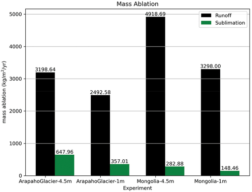
The mass ablation for a snow column for the canonical base cases for both Mongolia and Arapaho Glacier is shown in Figure 10. For 1-m snowfields, 4 percent of the Mongolian snowfield ablation was due to sublimation, whereas 13 percent of the Arapaho Glacier ablation was due to sublimation. The remainder was due to snow melt. For the 4.5-m cases, Mongolia snowfield’s ablation due to sublimation was 5 percent and Arapaho Glacier was 17 percent. Hence, overall, both Mongolia and Arapaho Glacier primarily lost mass due to snowmelt. However, the Mongolia perennial snowfields had less sublimation mass loss than Arapaho Glacier.

Figure 10. Total snowpack ablation amounts due to sublimation and melting for both snowfields in both locations. The amounts are shown for the base case. The Arapaho Glacier and Mongolia experiments were conducted with a 4.5-m snowpack.

Discussion

We can compare our results to previous work on glaciers and seasonal snowfields. These comparisons are useful because perennial snowfields fit between glaciers and seasonal snowfields in terms of climate conditions. Rupper and Roe (2008) analyzed the equilibrium line altitudes (ELAs) for glaciers in Central Asia and found that equilibrium line altitudes for glaciers in melt-dominated regions were more sensitive to air temperatures than those in sublimation dominated locations. That finding is consistent with our perennial snowfield model results as well, as shown in Figures 5 to 8. We found for both melt-dominated locations, as well as for both snowfield depths, that ablation was sensitive to increases in air temperatures. Snowpack ablation partitioning was as expected. Recall that Arapaho Glacier is located at a much higher elevation than the Ulaan Taiga site. Sublimation was greater both in absolute amounts as well as relative percentages of ablation at Arapaho Glacier. Similar to Rupper and Roe (2008), we found that Arapaho Glacier, being higher in elevation than the Mongolia snowfield, shows a greater sensitivity to precipitation.

Our results showing sensitivity of mass balance to air temperature are also consistent with previous work on seasonal snowpacks. In our 1-m case for Mongolia, we found that the constant warming scenario (2°C) resulted in the complete snowpack melt fourteen days earlier than in the base case. Similarly, for Arapaho Glacier we found the constant warming resulted in a 1-m snowpack disappearing twenty-six days earlier than in the base case. These results of our 1-m case are similar to the results of Clow (2010), who was studying seasonal snowpacks. Research by Clow (2010) has recently found that, for the Colorado Rocky Mountains, air temperature has been increasing and SWE of seasonal snowfields has been decreasing. Clow (2010) found that, from 1978 to 2007, November to May air temperatures increased by a median of 0.9°C/decade at U.S. Department of Agriculture Snow Telemetry sites in Colorado. At the same sites, Clow (2010) also found that 1 April SWE declined by a median of 4.1 cm/decade and maximum SWE declined by 3.6 cm/decade. At Niwot Ridge, a modeling study indicated each 1°C of warming is associated with alpine melt timing shifting 6.2 days earlier and a contraction of 10.7 days in the snow cover season (Jennings and Molotch 2020).

Dust deposition in our model occurs during the late summer. For the annual mass balance of a perennial snowfield, however, the key point is whether any snow survives the summer ablation. If it does, then the snow column will quickly become replenished in the fall/winter season. Note that for seasonal snowpacks, however, dust should have a large effect on meltout dates, because deposition would occur in the summer when the dwindling seasonal snowpacks are thin. Other research finds that dust and wildfire char deposition can markedly advance snowfield melt onset through reductions in snow surface albedo (Painter et al. 2017; Skiles and Painter 2017; Skiles et al. 2018; Gleason et al. 2019). Simulations indicate extreme dust loading (~4,000 ppm) can shift the snowmelt season three to six weeks earlier compared to moderate dust loading (Deems et al. 2013). Similarly, char deposition in a burned forest advanced complete snowpack melt by forty-seven days compared to snow in an unburned forest (Gleason, Nolin, and Roth 2013). Variations in wind speed and turbulent fluxes are known to drive patterns in snow persistence and disappearance in alpine catchments (Marks and Winstral 2001; Winstral, Elder, and Davis 2002; Mott et al. 2011; Dadic et al. 2013).

Dust deposition amounts have increased dramatically since the nineteenth century. Neff et al. (2008) found that dust loading in the Western United States has increased 500 percent over the late Holocene average since the nineteenth century. Snow cover duration has been found to be sensitive to dust content in the snow. Clow, Williams, and Schuster (2016) found that the amount of winter and spring dust deposition increased by 81 percent over 1993 to 2014. They also found that snowmelt initiation was accelerated seven to eighteen days by dust deposition on the snow surface. Painter et al. (2007) found that, for the San Juan mountains in southwestern Colorado, snow cover duration was shortened by eighteen to thirty-five days by the surface deposition of dust during the ablation season. Dust is prominent in the capital of Mongolia, Ulaanbaatar, which has extremely high concentrations of PM10. Though soot and other pollutants are both present, mineral dust particles are also in high abundance (Hasenkopf et al. 2016). For our 1-m case at Arapaho Glacier, we found that dust doubling shortened the snowpack lifetime by two days. The reason for the reduced lifetime seems to be the dust deposition occurred during July to September, a time when rainfall was occurring and altering the cold content of the snowpack. The 1-m dust-doubling case for Mongolia only resulted in a 1-hour shorter lifetime. Again, the occurrence of daily rain during the dust deposition season must account for a larger thermodynamic influence on the snowpack than the meager radiative forcing contribution from the dust doubling. It is possible that larger dust deposition events/amounts, similar to those observed by Clow, Williams, and Schuster (2016), would have more dramatic effects on perennial snowpack lifetimes, however.

A shortcoming of the model presented here is that our simplified scheme for snow deposition neglects the fact that blowing snow becomes less mobile as the melt season progresses. To quantify such effects would require a detailed coupled snow erosion model and thermal model and is beyond the scope of this study. In addition, we assume that the nivation hollows/cirques are accumulating windblown snow but losing snow via sublimation and melting; our model does not allow winds to remove snow from the hollow/cirque. It is certainly possible that the variables we study, such as wind speed, temperature, and precipitation, could themselves affect the snow deposition rates and hence the snowpack lifetimes. Those effects, however, are indirect effects in the sense that they arise from interactions among the variables. We do not investigate these effects in this study but hope to do so in future work.

Given the near-ubiquitous observed declines in seasonal snowpack water storage, perennial snowfield durations, and glacier mass balances (Hock et al. 2019), it is important to consider the downstream consequences of such losses. In the Western United States, streamflow is inextricably linked to SWE and snowmelt timing (Bales et al. 2006; Li et al. 2017), meaning that snowpack and snowfield changes manifest in streamflow variations (Stewart, Cayan, and Dettinger 2005; Stewart 2009). On Niwot Ridge, home to Arapaho Glacier, researchers posit that late-summer streamflow produced by melting glaciers and snowfields will decline over the decades ahead as these cryosphere features disappear (Leopold et al. 2015).

Conclusions

We have developed a detailed numerical model of the energy balance of perennial snowfields and use this to investigate annual net mass gain (or loss) from the snowfield resulting from changes in temperature, wind, dust influx, and precipitation. We applied the model to two perennial snowfields, Arapaho Glacier, located in the Colorado Rocky Mountains (United States), and a snowfield located in the Ulaan Taiga (Mongolia), both of which are used by local human populations and both of which are experiencing reductions in snow mass. The model incorporates year-round atmospheric data sets from each location.

From our analysis we draw the following conclusions:

First, we show that for these two locations the snowfield mass balance is primarily sensitive to air temperature and wind speed, followed by precipitation and dust deposition amounts.

Secondly, we find that the sensitivities are similar for the center of the snowfield as well as the margins.

Third, we find that the partitioning of ablation between sublimation and snowmelt are slightly different for the two sites. The higher elevation site, Arapaho Glacier, has a larger proportion of its ablation due to sublimation than the Mongolia site, which is at a lower elevation.

In particular, we conclude that the mass loss observed since the little ice age at the Arapaho Glacier, and much more recently at the Ulaan Taiga snowfield, is most likely due to increasing air temperatures.

This analysis of perennial snowfields could inform future investigations by emphasizing the role of sublimation losses in semi-arid continental montane climates. Much of the sublimation loss of perennial snowfields is driven by winds. Winds also replenish the snowfields by snow drifts, however, so the net effects are not obvious. Air temperature and humidity play important roles as well. Humidity, though correlated with precipitation, will factor prominently into sublimation losses. There is still important work to be done in the future. Understanding the complex relationship between timing of precipitation and dust deposition, immediate burial of dust by snow, or snow by dust, can likely have large implications in the overall longevity of snowfields. Clearly, more work remains to be done on these and other aspects of snowpack mass balance.

Acknowledgments

The authors thank David Clow (USGS) and Graham Sexstone (USGS) for their thoughtful comments and reviews.

Disclosure statement

No potential conflict of interest was reported by the authors.

Appendix 1:

Snowfield Model Description

The turbulent fluxes of sensible and latent heat have profound effects on the overall surface energy budget of the snow. Different approaches to computing these fluxes can result in large differences in calculated mass losses. We have modified the original snowfield model from Williams et al. (2008) and Heldmann et al. (2012) by introducing a more sophisticated treatment of the sensible and latent heat fluxes. The surface energy balance and model are described in both Williams et al. (2008) and Heldmann et al. (2012). Here we describe the new treatment of the sensible and latent heat turbulent fluxes, which the present snowfield model contains. In this model we use the formulations as outlined in Brock et al. (2000), where the turbulent sensible heat flux is given by

(A1)

and turbulent latent heat flux is

(A2)

where λ is the latent heat of vaporization of ice, C_p is the specific heat capacity of air at constant pressure, P is air pressure, z is the instrument height, T_z is air temperature at instrument height, T_s is the surface temperature, u_z is wind speed at instrument height, and L is the Monin-Obukhov length scale. Sublimation is calculated via the latent heat flux. The vapor pressure at the snow surface is given by e_s and the partial pressure at instrument height is given by e_z. The roughness length scales for momentum, temperature, and water vapor are designed by z₀, z_t, and z_e. The ratio of the molecular weight of water vapor to air is given by ω. The stability correction constants a_M, a_H, and a_E are for momentum, heat, and humidity, respectively, and are commonly assumed to be equal to five (Brock et al., 2000). We will discuss this value in the context of atmospheric stability.

The Monin-Obukhov length scale, L, is computed as

(A3)

where is the friction velocity, is air density, k is the Von Karman constant, g is acceleration due to gravity, and SH is the sensible heat calculated from Equation (A1).

The friction velocity is calculated as

(A4)

where a_x is another stability correction (where, again, ), and L is the length scale from Equation (A3).

Previous snow modeling literature has indicated issues with the Monin-Obukhov approach (Essery et al. 2013; Jennings et al, 2018); however, these issues are most likely the result of the difficulty of choosing stability corrections for the stable stratification regime. There has been considerable discussion in the literature regarding the appropriate values for the stability corrections “constants” a_M, a_H, a_E, and a_x, especially in the context of strongly stable atmospheres. Over snow and ice surfaces, the atmospheric profile is frequently stably stratified (Andreas 2002). For glacial surfaces, Brock et al. (2000) elected to use a constant value of five for all correction constants, regardless of atmospheric stability conditions. The work of Andreas (2002) suggests that, for stable conditions, the functional forms of Holtslag and DeBruin (1988) are recommended instead. In that formulation, we replace the terms containing , , and in the denominators of Equation (A1) and (A2) with the following stratification corrections for heat and momentum (Jordan, Andreas, and Makshtas 1999):

where the stratification parameter . In this case, we also make the substitution (Andreas 2002) of . Sexstone et al. (2016) used the same bulk formulation from Andreas (2002) and showed promising comparisons between this bulk formulation and sublimation fluxes measured by eddy covariance over a seasonal snowpack in Colorado. For unstable stratification, we retain the formulation with .

The value for the roughness length scales over snow and ice has also been debated in the literature, where a significant spread in values is found, ranging from 0.2 mm to 30 mm for snow surfaces (Brock, Willis, and Sharp 2006). The roughness length scales used in our model are taken from Brock, Willis, and Sharp (2006) and Munro (1989), where we use a value of 6.0 mm corresponding to “glacier snow” for all roughness length scales z₀, z_t, and z_e. As in Wagnon et al. (2003), we have treated the roughness length scales for heat, momentum, and vapor as equal. They are almost certainly not equal, but the investigation of the actual values is an involved undertaking that we hope to perform in the future.

Precipitation in the form of rain or snow was allowed to fall on the snowfield surface. We used a simple scheme to partition the precipitation into rain or snow. Precipitation was designated as rain when the wetbulb air temperature was greater than 0.5°C and designated as snow otherwise (Jennings et al. 2018).

The snow surface density in this study was assumed to be 500 kg/m³. This value was representative of wind-packed snow at Niwot Ridge (M. Williams, J. Morse, and Niwot Ridge LTER 2020). The snow density profile was initialized using the density profile of Paterson (1994) where the density ρ increases with depth z as

Here is the density of ice (917 kg/m³) and is the density of the surface snow (500 kg/m³ in this study). C is a constant for a given site, where in this case we used the value of 0.0246 m⁻¹ (Paterson 1994).

Appendix 2:

Model ResultsTable A1. Arapaho Glacier 4.5-m case.

Table

Experiments—Arapaho Glacier	Start mass (kg)	End mass (kg)	Change (%)
Base case	2,347.6	2,345.7	−0.08
Constant warming (2°C)	2,347.6	1,277.0	−45.60
Nighttime warming (0.25°C)	2,347.6	2,274.1	−3.13
Precipitation increase (1.22 times)	2,347.6	2,762.4	17.67
Wind decrease (0.82)	2,347.6	3,499.8	49.08
Dust increase (2 times)	2,347.6	2,295.5	−2.22

Table A2.

Mongolia 4.5-m case

Table

Experiments—Mongolia	Start mass (kg)	End mass (kg)	Change (%)
Base case	2,347.6	2,348.7	0.05
Constant warming (2°C)	2,347.6	1,452.8	−38.12
Nighttime warming (0.25°C)	2,347.6	2,307.5	−1.71
Precipitation increase (1.22 times)	2,347.6	2,430.1	3.51
Wind decrease (0.74)	2,347.6	3,161.3	34.66
Dust increase (2 times)	2,347.6	2,339.9	−0.33

Table A3.

Arapaho Glacier 1.0-m case

Table

Experiments—Arapaho Glacier	Start mass (kg) or base case lifetime	End mass (kg) or lifetime	Change (%)
Base case	247 days	247 days	0.00
Constant warming (2°C)	247 days	224 days	−0.09
Nighttime warming (0.25°C)	247 days	244 days	−0.01
Precipitation increase (1.22 times)	247 days	270 days	0.09
Wind decrease (0.82)	504.5 kg	1,574.8 kg	212.12
Dust increase (2 times)	247 days	245 days	−0.01

Table A4.

Mongolia 1.0-m case

Table

Experiments—Mongolia	Start mass (kg) or base case lifetime	End mass (kg) or lifetime	Change (%)
Base case	221 days	221 days	0.00
Constant warming (2°C)	221 days	207 days	−0.06
Nighttime warming (0.25°C)	221 days	220 days	0.00
Precipitation increase (1.22 times)	221 days	223 days	0.01
Wind decrease (0.74)	221 days	239 days	0.08
Dust increase (2 times)	221 days	221 days	0.00

Table A5.

Model sensitivity tests done with the Arapaho Glacier 4.5-m case

Table

Sensitivity tests—Arapaho Glacier	Start mass (kg)	End mass (kg)	Change (%)
Slope 30° to >20°	2,347.6	2,366.7	0.82
Aspect 90° to >100°	2,347.6	2,285.5	−2.65
Aspect 90° to >80°	2,347.6	2,407.3	2.54
Snow density 500 to >400 kg/m^3	1,922.0	1,970.1	2.50
Initial dust 1000 to >100 ppm	2,349.7	2,523.9	7.42
Ground density 1400 to >1600 kg/m^3	2,347.6	2,345.6	−0.08
Snow grain diameter 120 to >180 μm	2,347.6	2,239.3	−4.61
k_prime_ground 0.25 to >0.35 w/mK	2,347.6	2,345.5	−0.09

Appendix 3:

Model Validation Details

For model validation, the ablation rate and timing of our model was tested by comparison with our (a) Niwot Ridge Saddle data set and (b) model output from a popular and verified model: SNOWPACK (Lehning et al. 1999). Given an initial snow depth on 16 May 2017 of 1.71 m, SNOWPACK found that the snow completed melted away by 26 June 2017 at 21:00. Observations found it disappeared on 27 June 2017 at 04:00. Our model found the snowfield completed melted away on 25 June 2017 at 14:00 (7-hour difference from SNOWPACK and 14-hour difference from observations), using relatively clean snow (100 ppm dust), snow density 450 kg/m³, and 0.20-mm-diameter snow grains. The difference of 14 hours between our model result and the observed meltout is significantly smaller than the spread of snowfield modeling results in the literature for various models (for a given simulation, often differing by over one month; cf. Essery et al. 2013).

For model validation with Mongolia, a ground truth was not available; hence, we modeled the longevity of a dusty (1,000 ppm) 1-m snowpack (500 kg/m³) at the Ulaan Taiga location, emplaced on 1 January 2018. No snow drifting was included because we were just modeling an exposed snowfield on flat ground, not a perennial snowfield. The modeled meltout date was found to be 12 June 2018. The monthly area-averaged snow cover from MODIS of the Ulaan Taiga location showed meltout occurring in early June. Given numerous free parameters (e.g., initial snowpack density, dustiness of snow) of this modeling case, the correspondence between the MODIS data and the model output are within the range of the variations expected from the parameter uncertainties.

References

- Abu-Hamdeh, N. H., and R. C. Reeder. 2000. Soil thermal conductivity effects of density, moisture, salt concentration, and organic matter. Soil Science Society of America Journal 64:1285–90. doi:10.2136/sssaj2000.6441285x.
- Andreas, E. L. 2002. Parameterizing scalar transfer over snow and ice: A review. Journal of Hydrometeorology 3 (4):417–32. doi:10.1175/1525-7541(2002)003<0417:PSTOSA>2.0.CO;2.
- Baba, M. W., S. Gascoin, L. Jarlan, V. Simonneaux, and L. Hanich. 2018. Variations of the snow water equivalent in the Ourika Catchment (Morocco) over 2000–2018 using downscaled MERRA-2 data. Water 10 (9):1120. doi:10.3390/w10091120.
- Bales, R. C., N. P. Molotch, T. H. Painter, M. D. Dettinger, R. Rice, and J. Dozier. 2006. Mountain hydrology of the western United States. Water Resources Research 42 (8):W08432. doi:10.1029/2005WR004387.
- Batbaatar, J., A. R. Gillespie, D. Fink, A. Matmon, and T. Fujioka. 2018. Asynchronous glaciations in arid continental climate. Quaternary Science Reviews 182:1–19. doi:10.1016/j.quascirev.2017.12.001.
- Broberg, L. 2021. Relative snowpack response to elevation, temperature and precipitation in the Crown of the Continent region of North America 1980-2013. PLoS ONE 16 (4):e0248736. doi:10.1371/journal.pone.0248736.
- Brock, B. W., and N. S. Arnold. 2000. A spreadsheet-based (Microsoft Excel) point surface energy balance model for glacier and snowmelt studies. Earth Surface Processes and Landforms 25 (6):649–58. doi:10.1002/1096-9837(200006)25:6<649::AID-ESP97>3.0.CO;2-U.
- Brock, B. W., I. C. Willis, and M. J. Sharp. 2006. Measurement and parameterization of aerodynamic roughness length variations at Haut Glacier d’Arolla, Switzerland. Journal of Glaciology 52 (177):281–97. doi:10.3189/172756506781828746.
- Burns, S. P., N. P. Molotch, M. W. Williams, J. F. Knowles, B. Seok, R. K. Monson, A. A. Turnipseed, and P. D. Blanken. 2014. Snow temperature changes within a seasonal snowpack and their relationship to turbulent fluxes of sensible and latent heat. Journal of Hydrometeorology 15 (1):117–42. doi:10.1175/JHM-D-13-026.1.
- Caine, N. 1995. Snowpack influences on geomorphic processes in Green Lakes Valley, Colorado Front Range. Geographical Journal 161 (1):55–68. doi:10.2307/3059928.
- Chen, J., and A. Ohmura. 1990. Estimation of Alpine glacier water resources and their change since the 1870s. International Association of Hydrological Sciences 193.
- Clow, D. W. 2010. Changes in the timing of snowmelt and streamflow in Colorado: A response to recent warming. Journal of Climate 23 (9):1120–2306. doi:10.3390/w10091120.
- Clow, D. W., M. W. Williams, and P. F. Schuster. 2016. Increasing aeolian dust deposition to snowpacks in the Rocky Mountains inferred from snowpack, wet deposition, and aerosol chemistry. Atmospheric Environment 146:183–94. doi:10.1016/j.atmosenv.2016.06.076.
- Cox, D. T. C., I. M. D. Maclean, A. S. Gardner, and K. J. Gaston. 2020. Global variation in diurnal asymmetry in temperature, cloud cover, specific humidity and precipitation and its association with leaf area index. Global Change Biology 00:1–13. doi:10.1111/gcb.15336.
- Dadic, R., R. Mott, M. Lehning, M. Carenzo, B. Anderson, and A. Mackintosh. 2013. Sensitivity of turbulent fluxes to wind speed over snow surfaces in different climatic settings. Advances in Water Resources 55:178–89. doi:10.1016/j.advwatres.2012.06.010.
- Deems, J. S., T. H. Painter, J. J. Barsugli, J. Belnap, and B. Udall. 2013. Combined impacts of current and future dust deposition and regional warming on Colorado River Basin snow dynamics and hydrology. Hydrology and Earth System Sciences; Katlenburg-Lindau 17 (11):4401. doi:10.5194/hess-17-4401-2013.
- DeWalle, D., and A. Rango. 2008. Principles of snow hydrology. Cambridge: Cambridge University Press. doi:10.1017/CBO9780511535673.
- Dohrenwend, J. C. 1984. Nivation landforms in the western Great Basin and their paleoclimatic significance. Quaternary Research 22 (3):275–88.
- Dove, A., J. Heldmann, C. P. McKay, and O. B. Toon. 2012. Physics of a thick seasonal snowpack with possible implications for snow algae. Arctic, Antarctic, and Alpine Research 44 (1):36–49. doi:10.1657/1938-4246-44.1.36.
- Dozier, J., R. O. Green, A. W. Nolin, and T. H. Painter. 2009. Interpretation of snow properties from imaging spectrometry. Remote Sensing of Environment 113:S25–S37. doi:10.1016/j.rse.2007.07.029.
- Dunn, R. J. H. 2020. Global Climate. Bulletin of the American Meteorological Society Global Climate 101(8):S9–S128. Coauthors. doi:10.1175/BAMS-D-20-0104.1.
- Elder, K., J. Dozier, and J. E.-D.-M. Michaelsen. 1991. Snow accumulation and distribution in an alpine watershed. Water Resources Research 27 (7):1541–52.
- Essery, R., S. Morin, Y. Lejeune, and C. B. Ménard. 2013. A comparison of 1701 snow models using observations from an alpine site. Advances in Water Resources 55:131–48. doi:10.1016/j.advwatres.2012.07.013.
- Eyles, N., and L. Daurio. 2015. Little Ice Age debris lobes and nivation hollows inside Ubehebe Crater, Death Valley, California: Analog for Mars craters?. Geomorphology 245:231–42. doi:10.1016/j.geomorph.2015.05.029.
- Fassnacht, S. R., N. B. H. Venable, D. McGrath, and G. G. Patterson. 2018. Sub-seasonal snowpack trends in the Rocky Mountain National Park Area, Colorado, USA. Water 10:562. doi:10.3390/w10050562.
- Fountain, A. G., G. L. Dana, K. J. Lewis, B. H. Vaughn, and D. M. McKnight. 1998. Glaciers of the McMurdo Dry Valleys, southern Victoria Land, Antarctica. Ecosystem dynamics in a polar desert: The McMurdo Dry Valleys, Antarctica, 65–75. Washington, DC: American Geophysical Union.
- Fountain, A. G., B. Glenn, and H. J. Basagic. 2017. The geography of glaciers and perennial snowfields in the American West. Arctic, Antarctic, and Alpine Research 49 (3):391–410. doi:10.1657/AAAR0017-003.
- Fountain, A. G., T. H. Nylen, A. Monaghan, H. J. Basagic, and D. Bromwich. 2010. Snow in the McMurdo Dry Valleys, Antarctica. International Journal of Climatology: A Journal of the Royal Meteorological Society 30 (5):633–42. doi:10.1002/joc.1933
- Fujita, K., K. Hiyama, H. Iida, and Y. Ageta. 2010. Self‐regulated fluctuations in the ablation of a snow patch over four decades. Water Resources Research 46 (11). doi:10.1029/2009WR008383.
- Garwood, J. M., A. G. Fountain, K. T. Lindke, M. G. van Hattem, and H. J. Basagic. 2020. 20th Century retreat and recent drought accelerated extinction of mountain glaciers and perennial snowfields in the Trinity Alps, California. Northwest Science 94 (1):44–61. doi:10.3955/046.094.0104.
- Gascoin, S., S. Lhermitte, C. Kinnard, K. Bortels, and G. E. Liston. 2013. Wind effects on snow cover in Pascua-Lama, Dry Andes of Chile. Advances in Water Resources 55:25–39. doi:10.1016/j.advwatres.2012.11.013.
- Gelaro, R., W. McCarty, M. J. Suárez, R. Todling, A. Molod, L. Takacs, C. A. Randles, A. Darmenov, M. G. Bosilovich, and R. Reichle. 2017. The Modern-Era Retrospective Analysis for Research and Applications, Version 2 (MERRA-2). Advances in Water Resources 30:5419–54. Coauthors. doi:10.1175/JCLI-D-16-0758.1.
- Gleason, K. E., J. R. McConnell, M. M. Arienzo, N. Chellman, and W. M. Calvin. 2019. Four-fold increase in solar forcing on snow in western U.S. burned forests since 1999. Nature Communications 10 (1):2026. doi:10.1038/s41467-019-09935-y.
- Gleason, K. E., A. W. Nolin, and R. T. Roth. 2013. Charred forests increase snowmelt: Effects of burned woody debris and incoming solar radiation on snow ablation. Geophysical Research Letters 40 (17):4654–61. doi:10.1002/grl.50896.
- Goordial, J., A. Davila, D. Lacelle, W. Pollard, M. M. Marinova, C. W. Greer, J. DiRuggiero, C. P. McKay, and L. G. Whyte. 2016. Nearing the cold-arid limits of microbial life in permafrost of an upper dry valley, Antarctica. The ISME Journal 10 (7):1613–24. doi:10.1038/ismej.2015.239.
- Greenland, D. 1989. The climate of Niwot Ridge, Front Range, Colorado, U.S.A. Arctic and Alpine Research 21 (4):380–91. doi:10.1080/00040851.1989.12002751.
- Hansen, W. R., B. J. Chronic, and J. Matelock, 1978, Climatography of the Front Range urban corridor and vicinity, Colorado, USGS Professional Paper 1019.
- Hasenkopf, C. A., D. P. Veghte, G. P. Schill, S. Lodoysamba, M. A. Freedman, and M. A. Tolbert. 2016. Ice nucleation, shape, and composition of aerosol particles in one of the most polluted cities in the world: Ulaanbaatar, Mongolia. Atmospheric Environment 139:222–29. doi:10.1016/j.atmosenv.2016.05.037.
- Haugen, B. D., T. A. Scambos, W. T. Pfeffer, and R. S. Anderson. 2010. Twentieth-century changes in the thickness and extent of Arapaho Glacier, Front Range, Colorado. Arctic, Antarctic, and Alpine Research 42 (2):198–209. doi:10.1657/1938-4246-42.2.198.
- Hawkins, E., P. Ortega, E. Suckling, A. Schurer, G. Hegerl, P. Jones, M. Joshi, T. J. Osborn, V. Masson-Delmotte, J. Mignot, et al. 2017. Estimating changes in global temperature since the preindustrial period. Bulletin of the American Meteorological Society 98 (9):1841–56. doi:10.1175/BAMS-D-16-0007.1.
- Heindel, R. C., A. L. Putman, S. F. Murphy, D. A. Repert, and E.-L. S. Hinckley. 2020. Atmospheric dust deposition varies by season and elevation in the Colorado Front Range, USA. Journal of Geophysical Research: Earth Surface 125:e2019JF005436. doi:10.1029/2019JF005436
- Heldmann, J. L., M. Marinova, K. E. Williams, D. Lacelle, C. P. Mckay, A. Davila, W. Pollard, and D. T. Andersen. 2012. Formation and evolution of buried snowfield deposits in Pearse Valley, Antarctica, and implications for Mars. Antarctic Science 24 (3):299–316. doi:10.1017/S0954102011000903.
- Higuchi, K., T. Iozawa, Y. Fujii, and H. Kodama. 1980. Inventory of perennial snow patches in Central Japan. GeoJournal 4 (4):303–11. doi:10.1007/BF00219577.
- Hock, R., G. Rasul, C. Adler, B. Cáceres, S. Gruber, Y. Hirabayashi, M. Jackson, A. Kääb, S. Kang, S. Kutuzov, et al. 2019. Chapter 2: High Mountain Areas. IPCC Special Report on Ocean and Cryosphere in a Changing Climate. http://report.ipcc.ch/srocc/pdf/SROCC_FinalDraft_Chapter2.pdf.
- Holtslag, A. A. M., and H. A. R. de Bruin. 1988. Applied modeling of the nighttime surface energy balance over land. Journal of Meteorological Research 27 (6):689–704. doi:10.1175/1520-0450(1988)027<0689:AMOTNS>2.0.CO;2.
- Jennings, K. S., T. G. F. Kittel, and N. P. Molotch. 2018. Observations and simulations of the seasonal evolution of snowpack cold content and its relation to snowmelt and the snowpack energy budget. The Cryosphere 12 (5):1595–614. doi:10.5194/tc-12-1595-2018.
- Jennings, K. S., T. Kittel, and N. Molotch. 2019. Infilled climate data for C1, Saddle, and D1, 1990 - 2013, hourly. Environmental Data Initiative Dataset accessed 7/31/2020. doi:10.6073/pasta/1538ccf520d89c7a11c2c489d973b232.
- Jennings, K. S., and N. P. Molotch. 2020. Snowfall fraction, cold content, and energy balance changes drive differential response to simulated warming in an apline and subalpine snowpack. Frontiers in Earth Science 8:186. doi:10.3389/feart.2020.00186.
- Jennings, K. S., T. S. Winchell, B. Livneh, and N. P. Molotch. 2018. Spatial variation of the rain–snow temperature threshold across the Northern Hemisphere. Nature Communications 9(1):1148. doi:10.1038/s41467-018-03629-7.
- Jordan, R. E., E. L. Andreas, and A. P. Makshtas. 1999. Heat budget of snow-covered sea ice at North Pole 4. Journal of Geophysical Research 104 (C4):7785–806. doi:10.1029/1999JC900011.
- Karl, T. R., G. Kukla, V. N. Razuvayev, M. J. Changery, R. G. Quayle, R. R. Heim, et al. 1991. Global warming: Evidence for asymmetric diurnal temperature change. Geophysical Research Letters 18: 2253–56. doi:10.1029/91GL02900.
- Lehning, M., P. Bartelt, B. Brown, T. Russi, U. Stöckli, and M. Zimmerli. 1999. SNOWFIELD model calculations for avalanche warning based upon a new network of weather and snow stations. Cold Regions Science and Technology 30 (1–3):145–57. doi:10.1016/S0165-232X(99)00022-1.
- Lemke, P., J. Ren, R. B. Alley, I. Allison, J. Carrasco, G. Flato, Y. Fujii, G. Kaser, P. Mote, R. H. Thomas, and T. Zhang. 2007. Observations: Changes in snow, ice and frozen ground. In Climate Change 2007: The Physical Science Basis. Contribution of Working Group I to the Fourth Assessment Report of the Intergovernmental Panel on Climate Change, S. Solomon, D. Qin, M. Manning, Z. Chen, M. Marquis, K.B. Averyt, M. Tignor and H.L. Miller, eds., 337–84. Cambridge: Cambridge University Press.
- Leopold, M., G. Lewis, D. Dethier, N. Caine, and M. W. Williams. 2015. Cryosphere: Ice on Niwot Ridge and in the Green Lakes Valley, Colorado Front Range. Plant Ecology and Diversity 8 (5–6):625–38. doi:10.1080/17550874.2014.992489.
- Li, D., M. L. Wrzesien, M. Durand, J. Adam, and D. P. Lettenmaier. 2017. How much runoff originates as snow in the western United States, and how will that change in the future? Geophysical Research Letters 44 (12):6163–72. doi:10.1002/2017GL073551.
- Mahowald, N. M., S. Kloster, S. Engelstaedter, J. K. Moore, S. Mukhopadhyay, J. R. McConnell, S. Albani, et al. 2010. Observed 20th century desert dust variability: Impact on climate and biogeochemistry. Atmospheric Chemistry and Physics 10:10875–93. doi:10.5194/acp-10-10875-2010.
- Marks, D., and A. Winstral. 2001. Comparison of snow deposition, the snow cover energy balance, and snowmelt at two sites in a semiarid mountain basin. Journal of Hydrometeorology 2 (3):213–27. doi:10.1175/1525-7541(2001)002<0213:COSDTS>2.0.CO;2.
- McKay, C. P. 2009. Snow recurrence sets the depth of dry permafrost at high elevations in the McMurdo Dry Valleys of Antarctica. Antarctic Science 21 (1):89. doi:10.1017/S0954102008001508.
- McKay, C. P., G. D. Clow, D. T. Andersen, and R. A. Wharton Jr. 1994. Light transmission and reflection in perennially ice-covered Lake Hoare, Antarctica. Journal of Geophysical Research 99 (C10):20427–44. doi:10.1029/94JC01414.
- McVicar, T. R., M. L. Roderick, R. J. Donohue, L. T. Li, T. G. Van Niel, A. Thomas, J. Grieser, D. Jhajharia, Y. Himri, N. M. Mahowald, et al. 2012. Global review and synthesis of trends in observed terrestrial near-surface wind speeds: Implications for evaporation. Journal of Hydrology 416:182–205. doi:10.1016/j.jhydrol.2011.10.024.
- Meador, W. E., and W. R. Weaver. 1980. Two-stream approximations to radiative transfer in planetary atmospheres: A unified description of existing methods and a new improvement. Journal of the Atmospheric Sciences 37 (3):630–43. doi:10.1175/1520-0469(1980)037<0630:TSATRT>2.0.CO;2.
- Mote, P. W. 2003. Trends in snow water equivalent in the Pacific Northwest and their climatic causes. Geophysical Research Letters 30 (12):1601. doi:10.1029/2003GL017258.
- Mote, P. W. 2006. Climate-driven variability and trends in mountain snowpack in western North America. Journal of Climate 19 (23):6209–20. doi:10.1175/JCLI3971.1.
- Mott, R., L. Egli, T. Grünewald, N. Dawes, C. Manes, M. Bavay, and M. Lehning. 2011. Micrometeorological processes driving snow ablation in an Alpine catchment. The Cryosphere 5 (4):1083–98. doi:10.5194/tc-5-1083-2011.
- Mott, R., C. Gromke, T. Grünewald, and M. Lehning. 2013. Relative importance of advective heat transport and boundary layer decoupling in the melt dynamics of a patchy snow cover. Advances in Water Resources 55:88–97. doi:10.1016/j.advwatres.2012.03.001.
- Mott, R., V. Vionnet, and T. Grünewald. 2018. The seasonal snow cover dynamics: Review on wind-driven coupling processes. Frontiers in Earth Science 6:197. doi:10.3389/feart.2018.00197.
- Munro, D. S. 1989. Surface roughness and bulk heat transfer on a glacier: Comparison with eddy correlation. Journal of Glaciology 35 (121):343–48. doi:10.1017/S0022143000009266.
- Murphy, S. F. 2006. State of the Watershed: Water Quality of Boulder Creek, 34. Colorado: U.S. Geological Survey Circular 1284.
- Nandintsetseg, B., J. S. Greene, and C. E. Goulden. 2007. Trends in extreme daily precipitation and temperature near Lake Hövsgöl, Mongolia. International Journal of Climatology 27 (3):341–47. doi:10.1002/joc.1404.
- Nayak, A., D. Marks, D. G. Chandler, and M. Seyfried. 2010. Long-term snow, climate, and streamflow trends at the Reynolds Creek Experimental Watershed, Owyhee Mountains, Idaho, United States. Water Resources Research 46:W06519. doi:10.1029/2008WR007525.
- Neff, J., A. Ballantyne, G. Farmer, N. M. Mahowald, J. L. Conroy, C. C. Landry, J. T. Overpeck, T. H. Painter, C. R. Lawrence, and R. L. Reynolds, et al. 2008. Increasing eolian dust deposition in the western United States linked to human activity. Nature Geoscience 1(3):189–95. doi:10.1038/ngeo133.
- Ødegård, R. S., A. Nesje, K. Isaksen, M. A. Liss, T. Eiken, M. Schwikowski, and C. Uglietti. 2017. Climate change threatens archaeologically significant ice patches: Insights into their age, internal structure, mass balance and climate sensitivity. The Cryosphere 11 (1):17. doi:10.5194/tc-11-17-2017.
- Painter, T. H., A. P. Barrett, C. C. Landry, J. C. Neff, M. P. Cassidy, C. R. Lawrence, K. E. McBride, and G. L. Farmer. 2007. Impact of disturbed desert soils on duration of mountain snow cover. Geophysical Research Letters 34 (12):L12502. doi:10.1029/2007GL030284.
- Painter, T. H., M. G. Flanner, G. Kaser, B. Marzeion, R. A. VanCuren, and W. Abdalati. 2013. End of the Little Ice Age in the Alps forced by industrial black carbon. PNAS 110 (38):15216–21. doi:10.1073/pnas.1302570110.
- Painter, T. H., S. S. McKenzie, D. J. S, B. W. Tyler, and D. Jeff. 2017. Variation in rising limb of Colorado River snowmelt runoff hydrograph controlled by dust radiative forcing in snow. Geophysical Research Letters 45 (2):797–808. doi:10.1002/2017GL075826.
- Painter, T. H., S. M. Skiles, J. S. Deems, A. C. Bryant, and C. C. Landry. 2012. Dust radiative forcing in snow of the Upper Colorado River Basin: 1. A 6 year record of energy balance, radiation, and dust concentrations. Water Resources Research 48 (7):W07521. doi:10.1029/2012WR011985.
- Paterson, W. S. B. 1994. The Physics of Glaciers. 481. 3rd ed. Oxford: Butterworth-Heinemann.
- Patterson, E. M., D. A. Gillette, and B. H. Stockton. 1977. Complex index of refraction between 300 and 700 nm for Saharan aerosols. Journal of Geophysical Research 82 (21):3153–60. doi:10.1029/JC082i021p03153.
- Pierce, D. W., T. P. Barnett, H. G. Hidalgo, T. Das, C. Bonfils, B. D. Santer, G. Bala, M. D. Dettinger, D. R. Cayan, A. Mirin, et al. 2008. Attribution of declining western U.S. snowpack to human effects. Journal of Climate 21 (23):6425–44. doi:10.1175/2008JCLI2405.1.
- Pilø, L. H., J. H. Barrett, T. Eiken, E. Finstad, S. Grønning, J. R. Post-Melbye, A. Nesje, et al. 2021. Interpreting archaeological site-formation processes at a mountain ice patch: A case study from Langfonne, Norway. The Holocene 31 (3):469–82. doi:10.1177/0959683620972775.
- Pomeroy, J. W., and E. Brun. 2001. Snow Ecology: An Interdisciplinary Examination of Snow‐covered Ecosystems. In eds. H. G. Jones, J. W. Pomeroy, D. A. Walker, and R. Hoham, 378. Cambridge: Cambridge University Press.
- Rangwala, I., and J. R. Miller. 2012. Climate change in mountains: A review of elevation-dependent warming and its possible causes. Climatic Change 114 (3–4):527–47. doi:10.1007/s10584-012-0419-3.
- Reichle, R. H., C. S. Draper, Q. Liu, M. Girotto, S. P. P. Mahanama, R. D. Koster, and G. J. M. De Lannoy. 2017. Assessment of MERRA-2 land surface hydrology estimates. Journal of Climate 30 (8):2937–60. doi:10.1175/JCLI-D-16-0720.1.
- Rupper, S., and G. Roe. 2008. Glacier changes and regional climate: A mass and energy balance approach. Journal of Climate 21 (20):5384–401. doi:10.1175/2008JCLI2219.1.
- Schueler, T. 2000. The Compaction of Urban Soils: Technical Note #107 from Watershed Protection Techniques, Vol. 3, 661–65. Ellicott City, MD: Center for Watershed Protection.
- Schwerdtfeger, P. 1963. Theoretical derivation of the thermal conductivity and diffusivity of snow. International Association of Hydrological Sciences 61:75–81.
- Sexstone, G. A., D. W. Clow, S. R. Fassnacht, G. E. Liston, C. A. Hiemstra, J. F. Knowles, and C. A. Penn. 2018. Snow sublimation in mountain environments and its sensitivity to forest disturbance and climate warming. Water Resources Research 542 (2):1191–211. doi:10.1002/2017WR021172.
- Sexstone, G. A., D. W. Clow, D. I. Stannard, and S. R. Fassnacht, 2016. Comparison of methods for quantifying surface sublimation over seasonally snow-covered terrain. Hydrological Processes 30:3373–89. doi:10.1002/hyp.10864.
- Sherwood, S., M. J. Webb, J. D. Annan, K. C. Armour, P. M. Forster, J. C. Hargreaves, G. Hegerl, S. A. Klein, K. D. Marvel, E. J. Rohling, et al. 2020. An assessment of Earth’s climate sensitivity using multiple lines of evidence. Reviews of Geophysics 58 (4):e2019RG000678. doi:10.1029/2019RG000678.
- Skiles, S. M., M. Flanner, J. M. Cook, M. Dumont, and T. H. Painter. 2018. Radiative forcing by light-absorbing particles in snow. Nature Climate Change 8 (11):964. doi:10.1038/s41558-018-0296-5.
- Skiles, S. M., and T. Painter. 2017. Daily evolution in dust and black carbon content, snow grain size, and snow albedo during snowmelt, Rocky Mountains, Colorado. Journal of Glaciology 63 (237):118–32. doi:10.1017/jog.2016.125.
- Skiles, S. M., T. H. Painter, J. S. Deems, A. C. Bryant, and C. C. Landry, 2012. Dust radiative forcing in snow of the Upper Colorado River Basin: 2. Interannual variability in radiative forcing and snowmelt rates. Water Resources Research 48. doi: 10.1029/2012WR011986.
- Stewart, I. T. 2009. Changes in snowpack and snowmelt runoff for key mountain regions. Hydrological Processes 23 (1):78–94. doi:10.1002/hyp.7128.
- Stewart, I. T., D. R. Cayan, and M. D. Dettinger. 2005. Changes toward earlier streamflow timing across western North America. Journal of Climate 18 (8):1136–55. doi:10.1175/JCLI3321.1.
- Stigter, E. E., M. Litt, J. F. Steiner, P. N. J. Bonekamp, J. M. Shea, M. F. P. Bierkens, and W. W. Immerzeel. 2018. The importance of snow sublimation on a Himalayan Glacier. Frontiers in Earth Science 6:108. doi:10.3389/feart.2018.00108.
- Taylor, W., J. K. Clark, B. Reichhardt, G. W. L. Hodgins, J. Bayarsaikhan, O. Batchuluun, J. Whitworth, M. Nansalmaa, C. M. Lee, E. J. Dixon, et al. 2019. Investigating reindeer pastoralism and exploitation of high mountain zones in northern Mongolia through ice patch archaeology. PLoS ONE 14 (11):e0224741. doi:10.1371/journal.pone.0224741.
- Thorn, C. E. 1976. Quantitative evaluation of nivation in the Colorado Front Range. Geological Society of America Bulletin 87 (8):1169–78. Accessed August 26, 2020. doi:10.1130/0016-7606(1976)87<1169:QEONIT>2.0.CO;2.
- Toon, O. B., C. P. McKay, T. P. Ackerman, and K. Santhanam. 1989. Rapid calculation of radiative heating rates and photodissociation rates in inhomogeneous multiple scattering atmospheres. Journal of Geophysical Research 94:16287–301. doi:10.1029/JD094iD13p16287.
- United Nations. 2018. Third National Communication of Mongolia, 416pp. https://www4.unfccc.int/sites/SubmissionsStaging/NationalReports/Documents/06593841_Mongolia-NC3-2-Mongolia%20TNC%202018%20print%20version.pdf
- United Nations: United Nations Framework Convention on Climate Change. n. d. Initial National Communication: Mongolia [Internet]. https://unfccc.int/documents/125493
- Veettil, B. K., and U. Kamp. 2019. Global Disappearance of Tropical Mountain Glaciers: Observations, Causes, and Challenges. Geosciences 9 (5):196. Accessed August 26, 2020. doi:10.3390/geosciences9050196.
- Vuille, M., B. Francou, P. Wagnon, I. Juen, G. Kaser, B. G. Mark, and R. S. Bradley. 2008. Climate change and tropical Andean glaciers: Past, present and future. Earth-science Reviews 89 (3–4):79–96. doi:10.1016/j.earscirev.2008.04.002.
- Wagnon, P., J.-E. Sicart, E. Berthier, and J.-P. Chazarin. 2003. Wintertime high-altitude surface energy balance of a Bolivian glacier, Illimani, 6340 m above sea level. Journal of Geophysical Research 108 (D6):4177.
- Waldrop, H. A. 1964. Arapaho Glacier, a sixty-year record, University of Colorado Studies. Series in Geology 3:1–37.
- Warren, S. G. 1984. Optical constants of ice from the ultraviolet to the microwave. Applied Optics 23 (8):1206–25. doi:10.1364/AO.23.001206.
- Williams, M., J. Morse, and Niwot Ridge LTER. 2020. Snow cover profile data for Niwot Ridge and Green Lakes Valley, 1993 - ongoing. ver 15. Environmental Data Initiative Accessed 2020-10-22. doi:10.6073/pasta/a5fca9d02a4a6a0744cc0d0ffccacd09.
- Williams, K. E., O. Toon, J. Heldmann, C. McKay, and M. Mellon. 2008. Stability of mid-latitude snowfields on Mars. Icarus 196 (2):565–77. doi:10.1016/j.icarus.2008.03.017.
- Winstral, A., K. Elder, and R. E. Davis. 2002. Spatial snow modeling of wind-redistributed snow using terrain-based parameters. Journal of Hydrometeorology 3 (5):524–38. doi:10.1175/1525-7541(2002)003<0524:SSMOWR>2.0.CO;2.
- Wiscombe, W. J., and S. G. Warren. 1980. A model for the spectral albedo of snow. I: Pure snow. Journal of the Atmospheric Sciences 37 (12):2712–273. doi:10.1175/1520-0469(1980)037<2712:AMFTSA>2.0.CO;2.