Ecology of the diatom Aulacoseira pusilla in oligotrophic mountain lakes, with implications for paleoclimate reconstructions

ABSTRACT

Diatoms in lake sediments are used in paleoclimate reconstructions, particularly in treeless areas such as arctic and alpine regions. Some diatom species in the Aulacoseira group are often thought to bloom as lakes turnover (i.e., mix), suggesting links between these taxa and ice-out conditions. We investigated the distribution and ecology of Aulacoseira pusilla (Meister) Tuji & Houki 2004 in three high-elevation lakes of the U.S. Central Rocky Mountains. Vertical distributions of A. pusilla were quantified every three to four days shortly after the ice-out period for three weeks during July 2017. Populations from two of the lakes were incubated in situ in two experiments to assess the effects of Incubation depth × Nutrient additions and to quantify responses to light. In stratified conditions, the vertical distributions of this species varied spatially and temporally across the three lakes during the study period. There were blooms in the epilimnion of a moderately transparent lake and in deeper waters of a clear lake. Our results suggest that water transparency and its effects on light availability are important when defining relationships between this species and lake thermal conditions. Enhanced understanding of the ecology of A. pusilla will strengthen paleoclimate reconstructions using this species.

KEYWORDS:

• Aulacoseira pusilla
• light
• alpine
• lake thermal structure
• diatom autoecology

Introduction

The genus Aulacoseira Thwaites 1848 is considered cosmopolitan in distribution (Kociolek 2018), with the most recent report in Antarctic areas (Oaquim et al. 2017). Species within the genus grow as individual cells or form colonies joined by interlocking spines (Wehr, Sheath, and Kociolek 2015). They grow in lakes under a variety of conditions, from oligotrophic to eutrophic, acidic to alkaline, and clear to turbid. Taxa commonly associated with lower productivity lakes include A. pusilla, Aulacoseira distans (Ehrenberg) Simonsen 1979, Aulacoseira subarctica (Otto Müller) E.Y. Haworth 1990, Aulacoseira alpigena (Grunow) Krammer (1991), and Aulacoseira italica (Ehrenberg) Simonsen 1979. The seasonality of these taxa is controlled by thermal and nutrient stratification of lakes and these diatoms typically bloom during periods of enhanced mixing (Lund 1954, 1971; Jewson 1992; Carrick, Aldridge, and Schelske 1993; Reynolds and Irish 2006; Reynolds et al. 2002). Aulacoseira subarctica has been found to thrive in vertically mixed conditions, with a moderate concentration of nitrogen and phosphorus (Reynolds et al. 2002). The dense, heavily silicified cells are suspended with turbulent mixing, but with the development of stratification, the cells sink rapidly to the lake benthos. Once on the surface of the lake sediments, the cells may enter a vegetative resting form, where they persist until another mixing event (Sicko‐Goad, Stoermer, and Fahnenstiel 1986; McQuoid and Hobson 1996).

The relationship between Aulacoseira and lake mixing is used extensively in paleolimnological reconstructions. For example, extended lake mixing periods, increased turbulence, and later timing of ice-out have been inferred from increases in the relative abundances of various Aulacoseira taxa, with the effects of these factors on Aulacoseira ecology confirmed in some studies using contemporary water column patterns (Rühland et al. 2008; Wang et al. 2008; Solovieva et al. 2015). Using shifts in Aulacoseira densities as well as other diatom taxa, Stone, Saros, and Pederson (2016) constructed a diatom-inferred stratification index to identify periods of deep and shallow mixing in alpine and glacier lakes.

With the reliance on Aulacoseira taxa in many diatom-based paleoclimate reconstructions, further refinement of the association between these taxa and lake mixing is warranted owing to several issues. Though Aulacoseira taxa are a widespread and common member of lake phytoplankton, our understanding of the ecology of this group is based on a rather limited number of studies, which are primarily from low-elevation areas and are focused on quantifying the response of these species to environmental factors such as light, nutrients, or their interaction (Jewson, Rippey, and Gilmore 1981; Carrick, Aldridge, and Schelske 1993; Foy and Gibson 1993). Additional studies examining in situ distributions with changing lake thermal conditions would help to synthesize our understanding, particularly for alpine lakes. Lake mixing and thermal stratification affect phytoplankton distributions in part via light and nutrient conditions; gradients in these factors can be quite different in high-elevation compared to low-elevation lakes. High-elevation lakes are highly transparent compared to many low-elevation lakes, and relatively nutrient-rich deep waters can still be within the photic zone that supports algal production (Saros et al. 2005). This suggests that lake thermal conditions may shape resource availability and vertical habitat gradients differently in high- versus low-elevation lake systems.

Furthermore, the study of this group is challenging due to its morphological complexity; hence, information available for some species is used to make generalizations for the genus. For example, English and Potapova (2009) pointed out that misidentification of Aulacoseira taxa confounds the ecological understanding of this group and leads to unreliable environmental response relationships. The misidentification of similar species (Aulacoseira subborealis (G. Nygaard) Denys, Muylaert, and Krammer (2003)), A. subarctica, A. alpigena, Aulacoseira laevissima (Grunow) Krammer (1991), Aulacoseira nygaardii (Camburn) Camburn and Charles (2000), A. distans, Aulacoseira nivaloides (K. E. Camburn) English and Potapova (2009), Aulacoseira nivaloides (K.E.Camburn) English and Potapova (2009), and A. pusilla) leads to erroneous characterization of geographic distribution and ecological niche (Denys et al. 2003). For example, A. alpigena is associated with acidic oligotrophic environments, whereas A. pusilla, which is sometimes confused with A. alpigena, has been reported from a wide variety of trophic conditions (Denys et al. 2003; Leira 2005; Tuji 2015).

The objective of this research was to identify the environmental factors in alpine and subalpine oligotrophic lakes that control the occurrence and distribution of Aulacoseira pusilla, a relatively common taxon in mountain lakes of the Western United States (Williams et al. 2016; Spaulding et al. 2020). Specifically, we asked whether the occurrence and density of A. pusilla respond to water column stability or are a result of the interaction of physical aspects of the water column and nutrient availability. To address this question, the vertical and temporal distributions of A. pusilla were studied in the water columns of three high-elevation lakes of the Greater Yellowstone Area during July 2017. In situ microcosm experiments were used to assess the effects of nutrient availability, light access, and depth in the water column on the growth of this species. The findings of this study are significant because they provide information about the ecology of A. pusilla, a common but neglected planktonic taxon (Denys et al. 2003).

Methods

Site description

The Absaroka–Beartooth area is located in the central Rocky Mountains in Montana and Wyoming (Figure 1). The geology of this area is dominated by Precambrian granitic rock composed of Archean gneiss and accessory metamorphic rocks (Love and Christiansen 1985). The landscape is characteristic of the Greater Yellowstone Area, with alpine plateaus, U-shaped valleys, and tree lines ranging between 2,750 and 3,000 m above sea level (Saros et al. 2003). Because of the continental climate, the area has the lowest but longest snow accumulation (peaking in April) for the six ecoregions of the Western United States and the latest snowpack ablation season, which occurs around June (Trujillo and Molotch 2014). The region holds around 600 permanent alpine and subalpine lakes, characterized by low concentrations of phosphorus. The ice-free season in these lakes spans from early July to October.

Figure 1. Location of the study lakes.

Three lakes were selected for this study (Beauty Lake, Beartooth Lake, and Kersey Lake) based on previous research that indicated the presence of A. pusilla in these lakes (Spaulding et al. 2020; Saros, unpublished). Beauty (44.97° N, 109.57° W) and Beartooth (44.95° N, 109.60° W) lakes are situated at treeline, and Kersey (45.03° N, 109.84° W) lies in a forested watershed. The lakes are deep (>20 m) with small surface areas (<1 km²). The waters are oligotrophic, circumneutral (pH 6–7.6), and clear (1 percent attenuation depth for photosynthetically active radiation (Z_1percentPAR) is 10–17 m) and have low conductivity (7 to 30 µS cm⁻¹; Table 1).

Table 1. Select parameters of the study lakes

	Beauty	Beartooth	Kersey
Coordinates	44.97° N, 109.57° W	44.95° N, 109.6° W	45.95° N, 109.54° W
Altitude (m.a.s.l.)	2,874	2,713	2,460
Lake area (km^2)	0.36	0.45	0.47
ZMax (m)	35	26	21
Mixing depth (m)	4	5	5
Z1percentPAR (m)	>17	12.8	10
Nitrate (µM)	< 0.07	<0.07	< 0.07
TP (µM)	0.1	0.1	0.06
SRP (µM)	< 0.02	<0.02	<0.02
DSi (µM)	28.7	27.2	NA

Notes. Maximum depth (Z_Max), depth at which 1 percent of surface photosynthetically active radiation remains (Z_1percentPAR), total phosphorus (TP), soluble reactive phosphorus (SRP), and dissolved silica (DSi). NA = not available. Data from Saros et al. (2003, 2012) and Kessler et al. (2008).

Distribution patterns

The distributions of A. pusilla along the water column were assessed in each lake by surveying every three days between 11 to 28 July 2017. The sampling was limited to the period after ice-out, because high densities of Aulacoseira have been reported with lake turnover periods (Gibson, Anderson, and Haworth 2003) and sampling during the autumn turnover in these lakes is often not logistically feasible. Water was collected with a Van Dorn bottle every 3 m down to a depth of 15 m in Kersey Lake, 18 m in Beartooth Lake, and 21 m in Beauty Lake. The maximum depth of sampling was informed by relative differences in water clarity (e.g., Kersey Lake least transparent). Two 50-mL subsamples were collected from each depth and preserved with Lugol’s iodine for phytoplankton enumeration. Vertical profiles of temperature (°C), conductivity (SPC), dissolved oxygen (DO), and pH were measured with a YSI EXO2 multiparameter sonde at 1-m intervals down to a depth in the hypolimnetic zone of each lake where conditions remained constant. The identification of the epi-, meta-, and hypolimnion was determined by the temperature profile, based on the metalimnion as the zone in which temperature changed by ≥1°C per meter.

Water from each lake stratum was analyzed for total phosphorus (TP), total nitrogen (TN), soluble reactive phosphorus (SRP), dissolved organic carbon (DOC), nitrate (NO₃₋), ammonium (NH₄⁺), and dissolved silica (DSi). Water samples were collected from the middle of each lake stratum and held on ice until refrigeration was possible. Samples for the various dissolved nutrients and DOC were filtered with 25-mm Whatman GF/F filters (0.7-µm pore filter) prerinsed with deionized water, except DSi, which was filtered with polycarbonate filters (0.4-µm pore filter). Total nutrients were analyzed on whole water samples. TP and TN were determined using the persulfate digestion method (American Public Health Association (APHA) 2000). NO₃₋ was measured with the cadmium reduction method and NH₄⁺ with the phenate method. The nitrogen fractions were run on a Lachat QuickChem 8500 flow injection analyzer with a limit of quantification of 0.07 µM N for NO₃⁻, 0.14 µM N for NH₄⁺, and 0.7 µM N for TN. Values for NO₃⁻ and NH₄⁺ were added to determine dissolved inorganic nitrogen (DIN). SRP was analyzed with the ascorbic acid method. Both TP and SRP were analyzed on a Varian Cary-50 spectrophotometer, both with a limit of quantification of 0.06 µM P. DOC was measured using a Shimadzu TOC analyzer.

Light penetration in the water column was measured using a Secchi disc, approximating the Z_1percentPAR depth, assumed to be double the depth of the Secchi reading. The estimated values of Z_1percentPAR were used to calculate the vertical attenuation coefficient of light intensity (K_d) for each sampling date. The estimated average energy available for photosynthesis (PAR) in the epi-, meta-, or hypolimnion was calculated using the equation (Tilzer and Goldman 1978)

$I{ }_{Z_a\to Z_b}=\frac{I_0}{K_d\left(Z_b-Z_a\right)}\left(e^{-k_d{Z}_a}-e^{-k_d{Z}_b}\right),$

where Z_a is the depth at the top of the layer; Z_b is the depth at the bottom of the layer; I_o is irradiance at the surface, assumed to be equal to 1,800 µmol m⁻² s⁻¹, as measured for these lakes by Kessler et al. (2008); and K_d is the attenuation coefficient. The average estimated PAR is expressed in micromole (μmol) photons m⁻² s⁻¹, because it is the current unit to express the photosynthetic photon flux density available (Mottus et al. 2013). The thermal stability of the water column on each date in each lake was determined by calculating the relative thermal resistance (RTR) that measures the energy required to mix water of different densities (due to different temperatures; Birge 1910):

$RTR=\frac{\left(p2-p1\right){10}^6}{8},$

where p2 is the water density at the bottom using the average temperature in the hypolimnion for each sampling date and p1 is the water density at the surface using the average temperature in the epilimnion for each sampling date.

Phytoplankton samples from the vertical profiles were counted by the Utermöhl method (Edler and Elbrächter 2010) using 30 mL of each sample. The phytoplankton community was identified to genus level using appropriate sources (Wehr, Sheath, and Kociolek 2015) and enumerated with a Nikon TS-100 inverted microscope with 400× magnification. The community composition was established by counting one transect. This revealed that by the sampling time, A. pusilla was the only Aulacoseira present in the lakes; therefore, four additional transects were counted exclusively for the abundance of A. pusilla to improve the accuracy of these counts. One replicate per depth per sample date was counted. Because morphological similarities between low-mantle Aulacoseira species can lead to misidentification, different references were checked to compare diagnostic traits of similar species (Krammer and Lange-Bertalot 1991; Siver and Kling 1997; Camburn and Charles 2000). After discounting the presence of other Aulacoseira species, the identification of A. pusilla was confirmed with scanning electron microscopy observations, the information in Tuji (2015), and the original description found in Potapova (2010). Samples were cleaned using HCl and H₂O₂ (Battarbee 1973). Coverslips with dried sample slurries were mounted in Naphrax for light microscope observation at 1,000×, followed by scanning electron microscopy.

Experimental approaches

Two experiments were conducted to assess the response of A. pusilla to nutrients and/or light. The first experiment (E1) manipulated nutrients and incubation depth; the second one (E2) varied light exposure by incubation at a fixed depth in the water column (Supplementary Figure S1). The latter was conducted to isolate the effects of light from other factors (e.g., temperature) that could vary with the depth of incubation. Each experiment was conducted using natural A. pusilla populations, one from Beauty Lake and the other from Kersey Lake, to compare the response of the populations from both ecosystems. All experiments were incubated in Beauty Lake to ensure the same light and temperature conditions and because Beauty Lake has greater water clarity than Kersey Lake. Because lake stratification breaks the homogeneity created by mixing, we increased the possibilities of finding A. pusilla by collecting water from the three lake strata. For each lake, 5 L of water was collected from the middle of the epi-, meta-, and hypolimnion zones using a Van Dorn bottle to produce an integrated sample that was filtered with a 153-µm Nitex mesh to remove zooplankton. The integrated sample was used to fill the Falcon polystyrene 75-mL nontreated culture flasks that were used for the incubations in triplicate.

The effects of nutrients and incubation depth on A. pusilla growth and cell densities (E1) were assessed in a 2 × 3 experimental design that tested nutrient addition (N + P or no addition) and location in the water column (epi-, meta-, or hypolimnion). Nutrient additions were in the form of NaNO₃ (8 µM N) and NaH₂PO₄ (1 µM P). Flasks were incubated along an anchored rope attached to a buoy, with flasks placed into transparent Fisherbrand Bitran Specimen Storage Bags, which were then clipped onto the cord at 2-m (epilimnion), 8-m (metalimnion), or 15-m (hypolimnion) depth to position them in the appropriate zone. The incubation lasted eight days from 14 to 22 July. Onset HOBO Pendant sensors (UA-002-08) were used to track the temperature and relative light intensity at incubation depths. The sensors were attached to the ropes close to the experimental units at each depth.

The effect of light on A. pusilla growth and cell densities (E2) was assessed at 100 percent, 65 percent, and 25 percent of ambient PAR exposure. Flasks were incubated in the epilimnion at 2 m with light exposure unmodified (100 percent of ambient) or modified by covering the flasks with window screen (65 percent of ambient) or window screen + mesh bag (25 percent of ambient) according to the procedure described by Malik, Northington, and Saros (2017). Each flask was placed inside a transparent Bitran bag and clipped to an anchored rope. The containers were incubated for eight days (from 14 to 21 July). Two flasks per treatment were analyzed to evaluate the responses of the incubations.

Data analyses

Cell densities (cells mL⁻¹) were calculated using the number of cells counted and the volume examined. The total density for A. pusilla within each lake was calculated by the sum of densities of the epi-, meta-, or hypolimnion. The average pH, temperature, SPC, and DO were also calculated for each zone in each lake. The following analyses of these data were implemented in RStudio version 1.3.1 (RStudio Team 2020). Quantile–quantile plots and the Shapiro-Wilk test verified the normality in the distribution of the data using the R packages ggplot2 (Wickham 2016) and nortest (Gross and Ligges 2015), respectively. Because not all variables met the assumption of normality, package psych (Revelle 2019) was used to create a pair plot with Spearman’s rank order correlation including all of the variables. The analysis was repeated for each lake data set.

To understand the effect of the variables on the density of A. pusilla, we ran a regression analysis using generalized linear interactive modeling (GLIM). The continuous variables included for the GLIM were the biologically relevant factors identified from the Spearman’s rank order correlation. Even though we found variables that correlated to each other (light, temperature, pH, and DOC), variable selection was based on the physiological effect on phytoplankton. The GLIM was run using the log link and the Poisson distribution. The test was run separately for each lake given that relevant variables were different for each lake. Kersey and Beauty data included average values for conductivity (SPC), estimated photosynthetic photon flux density available (PAR), and nutrient concentration (TN, TP) in each zone (epi-, meta-, or hypolimnion) to test the association with A. pusilla density (den). For Beartooth Lake, the analysis was executed with SPC, TP, PAR, and ammonium (NH₄). The test was run without testing interactions between the terms. When overdispersion or underdispersion was detected using the package AER (Kleiber and Zeileis 2008), the distribution was adjusted with quasi-Poisson dispersion correction. The fitted model was generated by the removal of insignificant variables based on the effect on deviance and by checking the residuals using the package car for R (Fox and Weisberg 2019). The effect of the variables on the density of the taxon was graphed with the package jtools (Long 2019) using the standardized regression coefficients.

For each experiment, count data were transformed to density (cells mL⁻¹), and growth rates were calculated using the standard equation

$\mu =\frac{ln\left(F\right)-ln\left(I\right)}{T},$

where F is the final density, I is the initial density, and T is the number of incubation days. The values of density and growth rate for each set of experiments were graphically analyzed using box plots in the package ggplot2 (Wickham 2016) to detect trends for nutrient addition and incubation depth. Using the Shapiro-Wilk test and quantile–quantile plots, the normality assumption for density and growth rate was examined. Levene’s test in the package car (Fox and Weisberg 2019) was used to check the homogeneity of variance.

A two-way analysis of variance (ANOVA) was used to assess the effects of nutrients and incubation depth on growth rate, as well as cell densities. One-way ANOVA was used to evaluate the effect of light on density and growth rate in the light manipulation experiment. Both analyses were performed using the rstatix package for R (Kassambara 2020). Normality assumptions for each ANOVA were analyzed using model residuals. When the ANOVA showed significant effects, post hoc comparisons were executed (Tukey’s honestly significant difference) to identify which treatments or treatment levels showed statistical differences. The post hoc comparisons were run using the package agricolae (De Mendiburu 2020).

Results

Distribution patterns

Lake thermal structure was related to elevation. Kersey Lake, situated at the lowest elevation, was already thermally stratified when sampling began on 10 July (Figure 2A), with surface waters at 18°C and epilimnion depth (defined as the bottom of the epilimnion) at 2 m. Epilimnion depth ranged from 2 to 3 m over the sampling period; the limit of the metalimnion ranged from 7 to 9 m over the period. RTR values were higher (i.e., greater thermal stability) than those of the other two lakes and remained high throughout the sampling period (Supplementary Figure S2). Beartooth Lake, situated at an elevation between the other two lakes, was also already thermally stratified when sampling began on 11 July (Figure 2C), with surface waters at 13°C and epilimnion depth at 3 m. Epilimnion depth ranged from 2 to 3 m over the sampling period, and the limit of the metalimnion ranged from 5 to 8 m over the period. Finally, in Beauty Lake, situated at the highest elevation of the three lakes, initial surface temperatures on 11 July were around 9°C (Figure 2E), and the lake was not thermally stratified. By 14 July, the lake was weakly stratified at 5 m; epilimnion depths ranged from 2 to 3 m over the rest of the sampling period, and the limit of the metalimnion ranged from 5 to 7 m. RTR gradually increased over the sampling period (Supplementary Figure S2).

Figure 2. Temperature profile (colored contours) and Z_1percentPAR depth (solid pink line) on left-hand panels and vertical profile of the distribution of Aulacoseira pusilla on right-hand panels between 11 to 28 July 2017 in (A), (B) Kersey Lake, (C), (D) Beartooth Lake, and (E), (F) Beauty Lake.

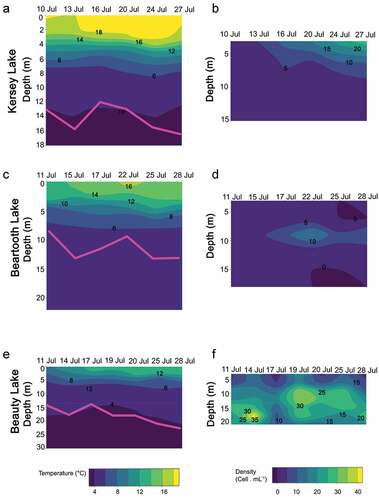
Water clarity was generally high but varied across all lakes. Calculated Z_1percentPAR for Kersey Lake suggests that the limit of the photic zone was between 12 and 14 m (Figure 2A). In Beartooth Lake, the estimated Z_1percentPAR was the lowest of the lakes, fluctuating around 10 m (Figure 2C). Water clarity was highest in Beauty Lake, with estimated Z_1percentPAR at 15 m or greater (Figure 2E).

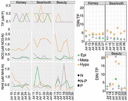
Nutrients were generally low during the observation period; the main fluctuations occurred along the lake strata and across all lakes (Figure 3, Supplementary Table SI). TP was <0.2 μM in all lakes, indicating oligotrophic systems. The lowest values were in Beauty Lake (0.1 μM). DIN was low but variable across lakes and zones (Supplementary Table SI). The lowest DIN concentrations were often in the epi- and metalimnion of all lakes, and the highest values were often found in the hypolimnion, but there were some exceptions, yielding highly variable DIN:TP over the sampling period (Figure 3). According to the DIN:TP ratio for oligotrophic lakes (Bergström 2010), in Kersey Lake, N and P co-limitation was often found in the epi- and metalimnion, except on 13 July, when N limitation was indicated. There were occasional indications of P limitation in these zones as well over the study period. The hypolimnion was the only layer that displayed a consistent pattern of P limitation during the study. In Beartooth Lake, limitation patterns appeared variable, but the hypolimnion always appeared P limited. DIN:TP and inferred limitation patterns were also variable in Beauty Lake.

Figure 3. Nutrient concentrations and ratios in Kersey, Beauty, and Beartooth lakes during the study. DIN:TP ratio calculated using concentrations in micrograms per liter. Geometric shapes indicate the type of nutrient limitation in each lake strata. Colors of geometric shapes identify the lake strata. Circles indicate N limitation, squares indicate P limitation, and triangles indicate N + P limitation.

The phytoplankton communities varied across the three lakes in both the relative abundance of phytoplankton groups and their vertical and temporal distributions (Figure 4 and Supplementary Figure S3). Aulacoseira pusilla comprised less than 5 percent of phytoplankton density, and Rhodomonas Karsten 1898 (Chrysophyseae) was frequently observed along the water column for all lakes.

Figure 4. Phytoplankton composition in Kersey, Beauty, and Beartooth lakes. (A) Percentage of the total cell density. Vertical distributions over time of the main phytoplankton taxa found in (B) Kersey Lake, (C) Beartooth Lake, and (D) Beauty Lake. Empty spaces in (D) correspond to the depths where the algae were not observed.

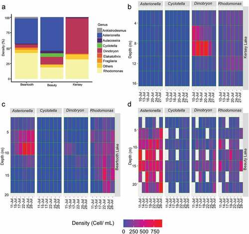
The Kersey Lake community was dominated by Dinobryon Ehrenberg 1834 (57 percent; Figure 4) and was found mainly between the meta- and hypolimnion (Figure 2), whereas A. pusilla was in the epilimnion. Beartooth Lake was co-dominated by Rhodomonas (42 percent) and Asterionella formosa Hassall 1850 (40 percent; Figure 4). The former was observed along the water column, and the latter was primarily concentrated between 5 and 10 m depth. Beauty Lake was dominated by Asterionella formosa (55 percent; Figure 4), which was present from the meta- to hypolimnion but mainly in the hypolimnion.

The densities and distributions of A. pusilla showed divergent patterns across the lakes (Figure 2). In Kersey Lake, cell densities oscillated between 0.3 and 29 cells mL⁻¹ and were low throughout the water column until mid-July, followed by a peak in the epilimnion (Figure 2B). The lowest densities of this diatom were found in Beartooth Lake, where the highest density occurred in the metalimnion during the second half of July (Figure 2D). Beauty Lake had the highest densities of any lakes (1.5–42 cells mL⁻¹; Figure 2F). Over the entire study period, the highest densities were found in the hypolimnion, but the peaks rose from a depth of 18 m at the beginning of the study to a range from 9 to 15 m from the middle to the end of the period. Microscopic examination of the cells revealed that in Kersey and Beauty lakes, chloroplasts were expanded, suggesting active cells, whereas some cells in the Beartooth Lake samples had contracted chloroplasts and may have been resting stages.

The regressions revealed that light was the common factor affecting the distributions of A. pusilla in all lakes (Supplementary Figure S3). In Kersey Lake, higher light had a positive impact on the density of A. pusilla (1.16e⁻³ ± 3.9e⁻⁴, p < .05). For Beauty (−1.8e⁻³ ± 1.3e⁻³, p < .001) and Beartooth (−4.9e⁻³ ±1.8 e⁻³, p < .05) lakes the effect of light was negative. In Beartooth Lake, low conductivity was also a significant factor (−0.45 ± 0.2, p < .001) for A. pusilla density. In Kersey and Beartooth lakes, models explained ~40 percent of the variability, and for Beauty Lake they explained 65 percent (Supplementary Table SII).

Results of experimental approaches

The average densities of A. pusilla at the beginning of the experiments for Kersey and Beauty lakes were 3.4 and 3.8 cells mL⁻¹, respectively. Average lake water chemistry at the time of collection of the experimental water and populations is provided in Tables 2 and 3. At the beginning of the experiments, DIN:TP ratio indicated that Kersey was N limited in the epi- and metalimnion and P limited in the hypolimnion. Beauty Lake was P limited. Silica concentration was low but sufficient in the epilimnion of both lakes (Kilham 1971).

Table 2. Average values of physical and chemical parameters in Kersey and Beauty Lake water samples used in the experiments

Lake	TN (µM N)	TP (µM P)	DIN (µM N)	SRP (µM P)	DOC (mM)
Kersey	7.4	0.2	0.8	0.02	250
Beauty	3.9	0.1	1.1	0.02	67

Table 3. Average temperature and irradiance in Beauty Lake for experiments incubated at different depths

Incubation zone	Temperature (°C)	Irradiance (μmol m^−2 s^−1)
Epilimnion (2 m)	12.5 ± 0.3	1,392
Metalimnion (8 m)	6 ± 0.1	525
Hypolimnion (15 m)	4 ± 0.02	97

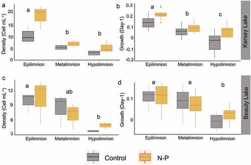
In the Nutrient × Incubation depth experiments, responses of A. pusilla populations from Kersey Lake (Figures 5A and 5B) and Beauty Lake (Figures 5C and 5D) were similar. Both populations had the highest cell densities and growth rates in the epilimnion incubations. The interaction of the nutrient addition and incubation depth did not influence the density or the growth rate in either lake. However, the effect of nutrients and incubation depth generated independent effects on the growth and density in populations from both lakes, but the magnitude of the effect and the importance of the factors were dissimilar for both populations. In Kersey Lake populations, nutrient addition explained 40 percent of the density values and 27 percent of the growth rate. Incubation depth explained 75 percent of the density values and 59 percent of growth rate. Post hoc comparisons revealed that density and growth rate for each nutrient treatment and incubation depth were statistically different between the epi- and hypolimnion. On the contrary, the metalimnion was only significantly different from the other lake strata for Kersey Lake population growth rate. In Beauty Lake populations, incubation depth was the only factor that had an effect on A. pusilla density, and it was responsible for 53 percent of the response in density and 43 percent of the growth rate. Nutrient addition was not significant for cell density or growth rate. Post hoc comparisons indicated that the greatest difference in densities occurred between the hypolimnion (4.1, ±0.81) and epilimnion (10.1, ±3.3). A similar pattern was observed for the growth rate between the epilimnion (0.11, ±0.05) and hypolimnion (7.7 e⁻³, ±0.04), whereas the growth rate in the metalimnion (0.07 ±0.06) was not different from that in the epilimnion. Based on these observations, we infer that the position in the water column is the most influential factor for both populations under these study conditions.

Figure 5. Response of Aulacoseira pusilla to incubation depth (epilimnion, metalimnion, hypolimnion) and nutrients (control, N + P) in bioassay experiments: (A) cell density and (B) growth rate in Kersey Lake populations; (C) cell density and (D) growth rate in Beauty Lake populations. Box ends are 25th and 75th percentiles; bold bars within boxes are 50th percentiles. Letters inside plots denote the results of post hoc analyses. Treatments with different letters indicate a significant difference between those treatments.

In the light experiments with Kersey Lake populations, there were no significant differences in cell densities across light levels (Table 4) but light had a positive effect as light access increased. Cell density and growth were low under dim conditions compared to the other treatments (Figure 6). Higher growth rates were apparent in the 100 percent and 65 percent ambient PAR treatments compared to those exposed to 25 percent ambient PAR. The ANOVA indicated significant differences in the growth rate of the light treatments, F (2, 24 = 3.4, p < .05, effect size 0.24. However, post hoc comparisons did not identify statistical differences between the treatments (100 percent PAR: 0.14 ± 0.04, 60 percent PAR: 0.13 ± 0.07, 25 percent PAR: 0.07 ± 0.05). There were logistical problems with the experiments with Beauty Lake populations (relative light intensity data on the HOBOs indicated that some flasks floated higher in the water column after anchoring), so the full sample set (n = 9, three samples per treatment) was discarded and not considered further.

Figure 6. The response of Aulacoseira pusilla from Kersey Lake populations to different levels of light expressed as a percentage of ambient (100 percent, 60 percent, or 25 percent) at 2-m depth: (A) density and (B) growth rate. Box ends are 25th and 75th percentiles; bold bars within boxes are 50th percentiles.

Table 4. Values of the results of ANOVA analyses for the Nutrients addition x incubation depths, and light access experiments for Kersey Lake and Beauty Lake populations

Experiment	Lake population	Factor	Parameter	Dfn	Dfd	F	p value	Effect size
Nutrient addition and incubation depth	Kersey	Interaction Nutrient^x incubation depth	Density	2	12	1.9	0.18	0.24
			Growth rate	2	48	1.26	0.3	0.05
		Nutrient	Density	2	12	8.1	<0.05	0.4
			Growth rate	1	48	18.16	<0.05	0.27
		Incubation depth	Density	2	12	18.2	<0.05	0.75
			Growth rate	2	48	34.3	<0.05	0.59
	Beauty	Interaction Nutrient^x incubation depth	Density	2	12	0.35	0.7	0.05
			Growth rate	2	48	1.25	0.2	0.05
		Nutrient	Density	1	12	0.01	>0.05
			Growth rate	1	48	5^x10-4	0.9
		Incubation depth	Density	2	12	6.85	<0.05	0.53
			Growth rate	2	48	18.5	<0.05	0.43
Light access	Kersey	Light level	Density	2	6	1.31	0.34	0.34
			Growth rate	2	24	3.4	<0.05	0.24

Discussion

With much prior research suggesting an association between Aulacoseira and lake mixing (Ilmavirta and Kotimaa 1974; Jewson, Rippey, and Gilmore 1981; Carrick, Aldridge, and Schelske 1993; Gibson, Anderson, and Haworth 2003; Pla et al. 2005) and our study starting with stratified lake conditions, we expected to find A. pusilla at deep zones of the three high-elevation lakes. As lakes stratify, nutrients decrease in shallow layers (Wetzel 2001), inducing higher densities of phytoplankton in deeper layers (Sommer 1984; Smetacek 1985; Larocque et al. 1996; Mellard et al. 2011). However, in this study, we found variable vertical distributions and small populations of A. pusilla. These findings contrast the expected abundance and pattern of distribution for stratified waters.

The effect of short colonies (two to four cells) and small cell size (7–10 µm diameter, 4–5 µm mantle height) found in this taxon may play a role in the observed distribution, affecting sinking losses (Reynolds 2006). A. pusilla is small compared to other Aulacoseira species such as A. lirata (6–23 µm diameter), A. italica (4–24 µm diameter), Aulacoseira valida (Grunow) Krammer (1991) (7–16 µm diameter), A. subarctica (3–14 µm diameter), and Aulacoseira granulata (Ehrenberg) Simonsen 1979 (4–17 µm diameter; Spaulding and Edlund 2008). Hence, the small size might decrease the sinking speed, explaining its nonexclusive distribution to the hypolimnion in these lakes.

The distribution along lake strata and temporal variation that we found across these three lakes during July 2017 suggests that for these populations of A. pusilla, water column stability did not control the vertical and temporal distributions. In Kersey Lake, the population appeared in the epilimnion during mid-summer thermally stratified conditions, whereas in Beauty Lake the population spread to the upper area of the hypolimnion even when the resistance to mixing was stronger by mid-summer. These distribution patterns, together with the experimental results, suggest the importance of light in shaping the response of this taxon. They also suggest that light requirements may vary across populations of A. pusilla based on ambient light and nutrient conditions. Specifically, in the same type of Nutrient × Incubation depth experiments, the Beauty Lake population was unaffected by nutrient enrichment, suggesting that it had access to nitrogen and phosphorus to support growth. This population grew equally well in the light conditions of the epi- and metalimnion. In contrast, growth of the Kersey Lake population was stimulated by nutrient addition. This response suggests nutrient-depleted conditions in Kersey Lake, supported by the frequent N and P co-limitation found in the epi- and metalimnion. Growth rates of this population in the incubations were greatest in the higher light conditions of the epilimnion, suggesting that nutrient depletion may have constrained growth at lower light intensities in the natural conditions of Kersey Lake. The differing light requirements of these two populations were also reflected in vertical distribution patterns of these two lakes during July. Collectively, these results suggest that for A. pusilla, as with many other diatom taxa (Malik and Saros 2016; Saros et al. 2016), relationships with lake physical features (e.g., mixing) are in part owing to links with effects on resource (light, nutrient) availability.

The distributions of other Aulacoseira taxa also highlight the importance of light in explaining distribution patterns (Jewson, Rippey, and Gilmore 1981; Gibson and Fitzsimons 1990; Foy and Gibson 1993; Gibson, Anderson, and Haworth 2003). Jewson et al. (2009) found that light attenuation regulates vertical distribution and growth rates of Aulacoseira baikalensis (Wisłouch) Simonsen (1979), diminishing its occurrence at shallow depths and at light intensities that induce inhibition but allowing its growth at deeper zones or optimal illumination. According to this, the observed vertical distribution patterns of A. pusilla are not only a product of sedimentation but also the effect of changes in light access. Light attenuation affects the distribution in the water column by reduction of the energy available, and sinking decreases exposure time as well. A. pusilla populations in Beauty Lake, regardless of location in the hypolimnion (less light exposure), were active (i.e., cells had expanded chloroplasts) and peaked and reached higher depths, further supporting that sinking alone was not the driver of these distribution patterns. Therefore, it is clear that the dynamics of A. pusilla are regulated by light exposure and complex water column stability factors (nutrient availability and location in water column), which we are only beginning to understand in freshwater systems.

The mechanisms that Aulacoseira taxa employ to control buoyancy are another facet of these dynamics and apparently were used in Beauty Lake, where an organic layer was observed on A. pusilla valves. Nutrient-depleted conditions in surface waters induce sinking by diatoms, which can promote the formation of a mucous secretion (Smetacek 1985). This organic layer facilitates sinking by aggregate formation; it can change to reduce sinking rates when there are enough nutrients available and appears when Aulacoseira are in a stationary phase (Smetacek 1985; Vieira et al. 2008). In Beauty Lake, we observed a thin organic layer on A. pusilla cells at greater depths, but it was not accompanied by aggregations or denser chain films. This suggests that these populations were employing this strategy to ensure the continuity of nutrient delivery to the cells by avoiding osmotic changes of nutrient concentration (Decho 1990; Karp-Boss, Boss, and Jumars 1996). The organic layer would not only ensure nutrient continuity but also regulate the sinking, as found in A. granulata cells, which modulated the stickiness, adherence, and aggregate size, formation, and settlement (Gibbs 1983; Decho 1990; Vieira et al. 2008). The experimental results support this theory, because Beauty Lake populations did not respond to nutrient additions, indicating sufficient nutrient access, because this lake was the last to stratify. This suggests that the deeper distributions of A. pusilla in Beauty Lake were likely controlled by a combination of nutrient availability due to late stratification onset, coupled with sufficient light. In contrast, the Kersey Lake pattern (late July bloom) may have been restricted to the higher light conditions of surface waters given the nutrient-depleted conditions. Studies of the effect of irradiance on phytoplankton sinking rate in Chaetoceros gracilis and C. flexuosum pointed out that sinking rates are lower in low-light environments than in higher light conditions, because the growth and photosynthesis in these environments occurs at a lower rate (Culver and Smith 1989).

Aulacoseira pusilla formed a relatively small fraction (<5 percent) of the total phytoplankton community in each lake. Lakes in this area tend to be dominated by Asterionella formosa as a consequence of enhanced N deposition in the region (Saros et al. 2005), with A. formosa blooms occurring shortly after ice-off in some lakes as a consequence of the pulse of N resulting from snowmelt, whereas in other lakes, blooms of this taxon are sustained over the short growing season (Figure 4), likely as a consequence of internal nutrient recycling. The dynamics of phytoplankton succession and the sequence of changes in Aulacoseira and A. formosa populations might reflect resource competition (Michel et al. 2006), whereas the dominance of Dinobryon and Rhodomonas in Kersey and Beartooth lakes coincided with reports in other alpine lakes that found them after the decrease of centric diatoms, associated with low P concentrations (Dokulil and Skolaut 1991; Marchetto et al. 2009).

With our sampling beginning shortly after ice-out but with thermal stratification at different stages, we may have missed earlier A. pusilla blooms in some of the lakes. In particular, Kersey Lake was already strongly stratified at the start of our sampling; as the lowest elevation lake in this study, ice-off was likely at least one to two weeks prior to our first sampling date. Regardless of earlier blooms in this lake, the late July bloom in the epilimnion suggested a population requiring relatively high light under the low-nutrient conditions present, which was further supported by the results of the light experiments (no nutrients were added in that set of experiments). The observation that Beauty Lake populations also shifted to shallower depths as summer progressed also supports this light and nutrient interplay, because these alpine lakes often receive a pulse of nitrogen with snowmelt, with the availability of that nitrogen rapidly declining within days to weeks after ice-out (Saros et al. 2005).

Prior research has indicated that A. pusilla may respond to nutrient enrichment (Denys et al. 2003; Williams et al. 2016). The 14 July peak in density in Beauty Lake coincided with high NO₃ concentration in the hypolimnion; this is consistent with observations from other alpine lakes in the United States where nitrogen enrichment stimulated the growth of this taxon (Williams et al. 2016). However, our GLIM result did not broadly corroborate the link across our samples. Indeed, we cannot suggest sensitivity for N or P because in our lakes, even though nutrient concentrations were highly variable temporally and spatially, we found no association between nutrients and A. pusilla density. Furthermore, the Nutrients × Incubation depth experiments did not indicate a consistent, positive effect on growth in both lakes. Different nutrient statuses for Kersey and Beauty samples likely shaped the results for both sets. These results largely revealed the interaction with physical factors that operate along the water column, affecting the growth of this species. Studying growth rate alone should not be used to provide information about algal physiological requirements, because the growth rate reflects the interaction between nutrient availability, light, and temperature (Rhee and Gotham 1981; Coles and Jones 2000; Staehr and Sand‐Jensen 2006).

Temperature is a factor that co-varied with light in both the distribution pattern studies and experiments and therefore may be a partial driver of observed patterns. In Kersey Lake, A. pusilla developed in warmer, high-light and nutrient-depleted conditions; meanwhile, in Beauty Lake, it thrived in cold, lower light, and moderate-nutrient waters. These contrasts in the initial conditions of the taxon at the onset of incubations showed that nutrient access is an important aspect that controls growth. However, there is a range of temperatures in which growth is not nutrient limited but temperature controlled. The growth lag at deeper depths of Kersey incubations and in Beauty samples suggests that suboptimal conditions for this species occurred below 6°C, whereas active cells observed in Kersey Lake suggest that temperatures ~20°C may still be optimal. Suboptimal temperature shapes nutrient demand and shifts abundance and growth in algal populations (Staehr and Sand‐Jensen 2006). Warm water temperature stimulates photosynthetic activity, nutrient demand, and growth; suboptimal thermal conditions slow nutrient uptake, affecting algal growth as well (Rhee and Gotham 1981; Davison 1991; Staehr and Sand‐Jensen 2006). Separating out the effects of temperature in future experiments would help to clarify the role of this factor further for A. pusilla populations.

Previous studies in Beauty Lake reported high abundance of A. pusilla (Stone, Saros, and Pederson 2016; Spaulding et al. 2020), in some ways contradicting our results, although those studies were on lake sediment records, which integrate diatom frustules over long time periods. The low density of A. pusilla that we observed in the water column suggests that we may have found what Smetacek (1985) defined as fugitive cells that found suitable conditions to persist in the water column and escaped the massive sinking and grazing effect of zooplankton. With most of the dominant phytoplankton characterized by large size colonies (A. formosa and Dinobryon), it is possible that size-selective zooplankton grazing was occurring (Leavitt, Carpenter, and Kitchell 1989). Large zooplankton graze on large or colonial algae, whereas small forms feed on small algae (Infante and Litt 1985). Future studies that include an assessment of grazing impacts would help to elucidate additional controls on A. pusilla populations.

Conclusions

The vertical distribution of A. pusilla in these alpine lakes showed different patterns, which, when coupled with the experimental observations, indicates that the occurrence and abundance of this species is not limited to deep zones once the resistance to mixing is established in lakes. Our results suggest that the distribution and abundance of A. pusilla are controlled by light and its interactions with nutrients and temperature. The fact that our study occurred under stratified conditions provides additional ecological understanding of this taxon and further information about population trends after lake mixing, filling gaps in our understanding of seasonal patterns. The study of A. pusilla in the time frame between mixing and stratification revealed the role of light and nutrients and shows the path that future research must address. Having more information in this regard will clarify the roles of different variables and address apparent contradictory inferences about the environments that favor A. pusilla (Denys et al. 2003; Tuji 2015; Williams et al. 2016). A deeper understanding of the ecology of this taxon will not only address gaps in autecological knowledge but also improve the prediction power of the taxon for paleolimnological studies, because we have provided information that shows that this taxon still thrives even in stratified conditions. Additionally, it would be interesting to further explore the role of the organic layer covering Aulacoseira as a regulatory strategy of this group to ensure favorable conditions, thereby expanding understanding about the ecology of this group after the mixing process.

Acknowledgments

We thank Jeffery Stone and three anonymous reviewers for comments on an earlier version of this article that helped to strengthen it.

Disclosure statement

No potential conflict of interest was reported by the authors.

Supplementary material

Supplemental material for this article can be accessed on the publisher’s website.

Additional information

Funding

We thank the Fulbright Commission in Colombia, the Minciencias–Fulbright scholarship, the Dan & Betty Churchill Exploration Fund (grant to ELPG), and the Gokcen Fund for the financial support. The help of the Diatom Ecology Lab members at the Climate Change Institute was essential to culminate different stages of this research.

References

- American Public Health Association (APHA). 2000. Standard methods for the examination of water and wastewater, 20.a ed. Washington, DC: APHA.
- Battarbee, R. W. 1973. A new method for estimating absolute microfossil numbers with special reference to diatoms. Limnology and Oceanography 18:647–53. doi:10.4319/lo.1973.18.4.0647.
- Bergström, A.-K. 2010. The use of TN: TP and DIN: TP ratios as indicators for phytoplankton nutrient limitation in oligotrophic lakes affected by N deposition. Aquatic Sciences 72 (3):277–81. doi:10.1007/s00027-010-0132-0.
- Birge, E. A. 1910. An unregarded factor in lake temperatures. Transactions of the Wisconsin Academy of Sciences 16:989–1004.
- Camburn, K. E., and D. F. Charles. 2000. Diatoms of low-alkalinity lakes in the northeastern United States.
- Carrick, H. J., F. J. Aldridge, and C. L. Schelske. 1993. Wind influences phytoplankton biomass and composition in a shallow, productive lake. Limnology and Oceanography 38 (6):1179–92. doi:10.4319/lo.1993.38.6.1179.
- Coles, J. F., and R. C. Jones. 2000. Effect of temperature on photosynthesis‐light response and growth of four phytoplankton species isolated from a tidal freshwater river. Journal of Phycology 36 (1):7–16. doi:10.1046/j.1529-8817.2000.98219.x.
- Culver, M. E., and W. O. Smith Jr. 1989. Effects of environmental variation on sinking rates of marine phytoplankton 1. Journal of Phycology 25 (2):262–70. doi:10.1111/j.1529-8817.1989.tb00122.x.
- Davison, I. R. 1991. Environmental effects on algal photosynthesis: Temperature. Journal of Phycology 27 (1):2–8. doi:10.1111/j.0022-3646.1991.00002.x.
- De Mendiburu, F. 2020. Agricolae: statistical procedures for agricultural research. (1.3-3) [computer software]. https://CRAN.R-project.org/package=agricolae
- Decho, A. W. 1990. Microbial exopolymer secretions in ocean environments: Their role (s) in food webs and marine processes. Oceanography and Marine Biology: An Annual Review 28 (7):73–153.
- Denys, L., K. Muylaert, K. Krammer, T. Joosten, M. Reid, and P. Rioual. 2003. Aulacoseira subborealis stat. Nov. (Bacillariophyceae): A common but neglected plankton diatom. Nova Hedwigia 77 (3–4):407–27. doi:10.1127/0029-5035/2003/0077-0407.
- Dokulil, M. T., and C. Skolaut. 1991. Aspects of phytoplankton seasonal succession in Mondsee, Austria, with particular reference to the ecology of Dinobryon Ehrenb. Internationale Vereinigung für theoretische und angewandte Limnologie: Verhandlungen 24 (2):968–73.
- Edler, L., and M. Elbrächter. 2010. The Utermöhl method for quantitative phytoplankton analysis. Microscopic and Molecular Methods for Quantitative Phytoplankton Analysis 110:13–20.
- English, J., and M. Potapova. 2009. Aulacoseira pardata sp. Nov., A. nivalis comb. Nov., A. nivaloides comb. Et stat. Nov., and their occurrences in Western North America. Proceedings of the Academy of Natural Sciences of Philadelphia 158 (1):37–48. doi:10.1635/053.158.0102.
- Fox, J., and S. Weisberg. 2019. An R Companion to Applied Regression, 3rd ed. Thousand Oaks, CA: Sage Publications.
- Foy, R., and C. Gibson. 1993. The influence of irradiance, photoperiod and temperature on the growth kinetics of three planktonic diatoms. European Journal of Phycology 28 (4):203–12. doi:10.1080/09670269300650311.
- Gibbs, R. J. 1983. Effect of natural organic coatings on the coagulation of particles. Environmental Science & Technology 17 (4):237–40. doi:10.1021/es00110a011.
- Gibson, C. E., and A. Fitzsimons. 1990. Induction of the resting phase in the planktonic diatom Aulacoseira subarctica in very low light. British Phycological Journal 25 (4):329–34. doi:10.1080/00071619000650361.
- Gibson, C. E., N. J. Anderson, and E. Y. Haworth. 2003. Aulacoseira subarctica: Taxonomy, physiology, ecology and palaeoecology. European Journal of Phycology 38 (2):83–101. doi:10.1080/0967026031000094102.
- Gross, J., and U. Ligges. 2015. Nortest: Tests for normality. (1.0-4) [computer software]. https://CRAN.R-project.org/package=nortest
- Ilmavirta, K., and A.-L. Kotimaa. 1974. Spatial and seasonal variations in phytoplanktonic primary production and biomass in the oligotrophic lake Pääjärvi, southern Finland. Annales Botanici Fennici 11(2):112–20.
- Infante, A., and A. H. Litt. 1985. Differences between two species of Daphnia in the use of 10 species of algae in Lake Washington 1. Limnology and Oceanography 30 (5):1053–59. doi:10.4319/lo.1985.30.5.1053.
- Jewson, D., B. Rippey, and W. Gilmore. 1981. Loss rates from sedimentation, parasitism, and grazing during the growth, nutrient limitation, and dormancy of a diatom crop. Limnology and Oceanography 26 (6):1045–56. doi:10.4319/lo.1981.26.6.1045.
- Jewson, D. 1992. Size reduction, reproductive strategy and the life cycle of a centric diatom. Philosophical Transactions of the Royal Society of London. Series B, Biological Sciences 336 (1277):191–213.
- Jewson, D. H., N. G. Granin, A. A. Zhdanov, and R. Y. Gnatovsky. 2009. Effect of snow depth on under-ice irradiance and growth of Aulacoseira baicalensis in Lake Baikal. Aquatic Ecology 43 (3):673–79. doi:10.1007/s10452-009-9267-2.
- Karp-Boss, L., E. Boss, and P. Jumars. 1996. Nutrient fluxes to planktonic osmotrophs in the presence of fluid motion. Oceanography and Marine Biology 34:71–108.
- Kassambara, A. 2020. Rstatix: Pipe-friendly framework for basic statistical tests. R package version 0.4. 0.
- Kessler, K., R. S. Lockwood, C. E. Williamson, and J. E. Saros. 2008. Vertical distribution of zooplankton in subalpine and alpine lakes: Ultraviolet radiation, fish predation, and the transparency‐gradient hypothesis. Limnology and Oceanography 53 (6):2374–82. doi:10.4319/lo.2008.53.6.2374.
- Kilham, P. 1971. A hypothesis concerning silica and the freshwater planktonic diatoms 1. Limnology and Oceanography 16 (1):10–18. doi:10.4319/lo.1971.16.1.0010.
- Kleiber, C., and A. Zeileis. 2008. Applied econometrics with R. New York: Springer-Verlag. https://CRAN.R-project.org/package=AER.
- Kociolek, J. 2018. A worldwide listing and biogeography of freshwater diatom genera: A phylogenetic perspective. Diatom Research 33 (4):509–34. doi:10.1080/0269249X.2019.1574243.
- Krammer, K., and H. Lange-Bertalot. 1991. Bacillariophyceae. 4. Teil: Achnanthaceae. Süsswasserflora von Mitteleuropa. Band 2/4. Stuttgart, Jena: Fischer, 1991b.–437
- Larocque, I., A. Mazumder, M. Proulx, D. R. Lean, and F. Pick. 1996. Sedimentation of algae: Relationships with biomass and size distribution. Canadian Journal of Fisheries and Aquatic Sciences 53 (5):1133–42. doi:10.1139/f96-025.
- Leavitt, P., S. Carpenter, and J. Kitchell. 1989. Whole‐lake experiments: The annual record of fossil pigments and zooplankton. Limnology and Oceanography 34 (4):700–17. doi:10.4319/lo.1989.34.4.0700.
- Leira, M. 2005. Diatom responses to Holocene environmental changes in a small lake in northwest Spain. Quaternary International 140:90–102. doi:10.1016/j.quaint.2005.05.005.
- Long, J. A. 2019. Jtools: Analysis and presentation of social scientific data. (2.0.1) [computer software]. https://cran.r-project.org/package=jtools>
- Love, J. D., and A. C. Christiansen. 1985. Geologic map of Wyoming. Denver, CO: U.S. Geological Survey. doi:10.3133/70046739.
- Lund, J. 1954. The seasonal cycle of the plankton diatom, Melosira italica (Ehr.) Kutz. Subsp. subarctica O. Mull. The Journal of Ecology 42:151–79. doi:10.2307/2256984.
- Lund, J. 1971. An artificial alteration of the seasonal cycle of the plankton diatom Melosira italica subsp. subarctica in an English lake. The Journal of Ecology 59 (2):521–33. doi:10.2307/2258329.
- Malik, H. I., and J. E. Saros. 2016. Effects of temperature, light and nutrients on five Cyclotella sensu lato taxa assessed with in situ experiments in Arctic lakes. Journal of Plankton Research 38 (3):431–42. doi:10.1093/plankt/fbw002.
- Malik, H. I., R. M. Northington, and J. E. Saros. 2017. Nutrient limitation status of Arctic lakes affects the responses of Cyclotella sensu lato diatom species to light: Implications for distribution patterns. Polar Biology 40 (12):2445–56. doi:10.1007/s00300-017-2156-6.
- Marchetto, A., M. Rogora, A. Boggero, S. Musazzi, A. F. Lotter, A. Lami, M. Tolotti, H. Thies, R. Psenner, J. Massaferro, et al. 2009. Response of alpine lakes to major environmental gradients, as detected through planktonic, benthic and sedimentary assemblages. Advances in Limnology 62:419–40. doi:10.1127/advlim/62/2009/419.
- McQuoid, M. R., and L. A. Hobson. 1996. Diatom resting stages. Journal of Phycology 32 (6):889–902. doi:10.1111/j.0022-3646.1996.00889.x.
- Mellard, J. P., K. Yoshiyama, E. Litchman, and C. A. Klausmeier. 2011. The vertical distribution of phytoplankton in stratified water columns. Journal of Theoretical Biology 269 (1):16–30. doi:10.1016/j.jtbi.2010.09.041.
- Michel, T. J., J. E. Saros, S. J. Interlandi, and A. P. Wolfe. 2006. Resource requirements of four freshwater diatom taxa determined by in situ growth bioassays using natural populations from alpine lakes. Hydrobiologia 568 (1):235–43. doi:10.1007/s10750-006-0109-0.
- Mottus, M., M. Sulev, F. Baret, A. Reinart, and R. Lopez. 2013. Photosynthetically active radiation: Measurement and modeling. In Solar Energy, 140–69. New York, NY: Springer. https://link.springer.com/content/pdf/10.1007/978-1-4614-5806-7.pdf
- Oaquim, A. B. J., G. A. Moser, H. Evangelista, M. V. Licínio, and B. Van De Vijver. 2017. Aulacoseira glubokoyensis sp. nov. (Bacillariophyceae), a new centric diatom from the maritime Antarctic region. Phytotaxa 328 (2):149–58. doi:10.11646/phytotaxa.328.2.5.
- Pla, S., A. M. Paterson, J. P. Smol, B. J. Clark, and R. Ingram. 2005. Spatial variability in water quality and surface sediment diatom assemblages in a complex lake basin: Lake of the woods, Ontario, Canada. Journal of Great Lakes Research 31 (3):253–66.
- Potapova, M. 2010. Aulacoseira pusilla. Diatoms of North America. https://diatoms.org/species/aulacoseira_pusilla.
- Revelle, W. 2019. Psych: Procedures for personality and psychological research, (1.9.12.) [computer software]. Northwestern University. https://CRAN.R-project.org/package=psych
- Reynolds, C. S. 2006. The Ecology of Phytoplankton. Ecology, Biodiversity and Conservation. Cambridge: Cambridge University Press. https://books.google.com/books?id=gDz5jGsPWZYC.
- Reynolds, C. S., V. Huszar, C. Kruk, L. Naselli-Flores, and S. Melo. 2002. Towards a functional classification of the freshwater phytoplankton. Journal of Plankton Research 24 (5):417–28. doi:10.1093/plankt/24.5.417.
- Reynolds, C. S., and A. Irish. 1997. Modelling phytoplankton dynamics in lakes and reservoirs: The problem of in-situ growth rates. Hydrobiologia 349 (1–3):5–17. doi:10.1023/A:1003020823129.
- Rhee, G.-Y., and I. J. Gotham. 1981. The effect of environmental factors on phytoplankton growth: Light and the interactions of light with nitrate limitation 1. Limnology and Oceanography 26 (4):649–59. doi:10.4319/lo.1981.26.4.0649.
- RStudio Team. 2020. RStudio: Integrated development environment for R. Boston, MA: Citeseer. http://www.rstudio.com/.
- Rühland, K., A. M. Paterson, and J. P. Smol. 2008. Hemispheric‐scale Patterns of Climate‐related Shifts in Planktonic Diatoms from North American and European Lakes. Global Change Biology 14 (11):2740–54. doi:10.1111/j.1365-2486.2008.01670.x.
- Saros, J. E., S. J. Interlandi, A. P. Wolfe, and D. R. Engstrom. 2003. Recent changes in the diatom community structure of lakes in the Beartooth mountain range, USA. Arctic, Antarctic, and Alpine Research 35 (1):18–23. doi:10.1657/1523-0430(2003)035[0018:RCITDC]2.0.CO;2.
- Saros, J. E., T. J. Michel, S. J. Interlandi, and A. P. Wolfe. 2005. Resource requirements of Asterionella formosa and Fragilaria crotonensis in oligotrophic alpine lakes: Implications for recent phytoplankton community reorganizations. Canadian Journal of Fisheries and Aquatic Sciences 62 (7):1681–89. doi:10.1139/f05-077.
- Saros, J. E., J. R. Stone, G. T. Pederson, K. E. Slemmons, T. Spanbauer, A. Schliep, D. Cahl, C. E. Williamson, and D. R. Engstrom. 2012. Climate‐induced changes in lake ecosystem structure inferred from coupled neo‐and paleoecological approaches. Ecology 93 (10):2155–64. doi:10.1890/11-2218.1.
- Saros, J. E., R. M. Northington, D. S. Anderson, and N. J. Anderson. 2016. A whole‐lake experiment confirms a small centric diatom species as an indicator of changing lake thermal structure. Limnology and Oceanography Letters 1 (1):27–35. doi:10.1002/lol2.10024.
- Sicko‐Goad, L., E. F. Stoermer, and G. Fahnenstiel. 1986. Rejuvenation of Melosira granulata (Bacillariophyceae) resting cells from the anoxic sediments of Douglas Lake, Michigan. I. Light migroscopy and 14C uptake 1. Journal of Phycology 22 (1):22–28. doi:10.1111/j.1529-8817.1986.tb02510.x.
- Siver, P. A., and H. Kling. 1997. Morphological observations of Aulacoseira using scanning electron microscopy. Canadian Journal of Botany 75 (11):1807–35. doi:10.1139/b97-894.
- Smetacek, V. 1985. Role of sinking in diatom life-history cycles: Ecological, evolutionary and geological significance. Marine Biology 84 (3):239–51. doi:10.1007/BF00392493.
- Solovieva, N., A. Klimaschewski, A. E. Self, V. Jones, E. Andrén, A. A. Andreev, D. Hammarlund, E. Lepskaya, and L. Nazarova. 2015. The Holocene environmental history of a small coastal lake on the north-eastern Kamchatka Peninsula. Global and Planetary Change 134:55–66. doi:10.1016/j.gloplacha.2015.06.010.
- Sommer, U. 1984. Sedimentation of principal phytoplankton species in Lake Constance. Journal of Plankton Research 6 (1):1–14. doi:10.1093/plankt/6.1.1.
- Spaulding, S., and M. Edlund. 2008. Aulacoseira. Diatoms of the United States. http://westerndiatoms.colorado.edu/taxa/genus/Aulacoseira
- Spaulding, S. A., J. R. Stone, S. A. Norton, A. Nurse, and J. E. Saros. 2020. Paleoenvironmental context for the Late Pleistocene appearance of Didymosphenia in a North American alpine lake. Aquatic Sciences 82 (1):10.
- Staehr, P. A., and K. Sand‐Jensen. 2006. Seasonal changes in temperature and nutrient control of photosynthesis, respiration and growth of natural phytoplankton communities. Freshwater Biology 51 (2):249–62. doi:10.1111/j.1365-2427.2005.01490.x.
- Stone, J. R., J. E. Saros, and G. T. Pederson. 2016. Coherent late-Holocene climate-driven shifts in the structure of three Rocky Mountain lakes. The Holocene 26 (7):1103–11. doi:10.1177/0959683616632886.
- Tilzer, M. M., and C. R. Goldman. 1978. Importance of mixing, thermal stratification and light adaptation for phytoplankton productivity in Lake Tahoe (California‐Nevada). Ecology 59 (4):810–21. doi:10.2307/1938785.
- Trujillo, E., and N. P. Molotch. 2014. Snowpack regimes of the western United States. Water Resources Research 50 (7):5611–23. doi:10.1002/2013WR014753.
- Tuji, A. 2015. Distribution and taxonomy of the Aulacoseira distans species complex found in Japanese harmonic artificial reservoirs. Bulletin of the National Museum of Nature and Science Series B (Botany) 41:53–60.
- Vieira, A. A., P. I. Coelho Ortolano, D. Giroldo, M. J. Dellamano Oliveira, T. B. Bittar, A. T. Lombardi, A. L. Sartori, and B. S. Paulsen. 2008. Role of hydrophobic extracellular polysaccharide of Aulacoseira granulata (Bacillariophyceae) on aggregate formation in a turbulent and hypereutrophic reservoir. Limnology and Oceanography 53 (5):1887–99. doi:10.4319/lo.2008.53.5.1887.
- Wang, L., H. Lu, J. Liu, Z. Gu, J. Mingram, G. Chu, J. Li, P. Rioual, J. F. W. Negendank, and J. Han. 2008. Diatom‐based Inference of Variations in the Strength of Asian Winter Monsoon Winds between 17,500 and 6000 Calendar Years BP. Journal of Geophysical Research: Atmospheres 113 (D21). doi:10.1029/2008JD010145.
- Wehr, J. D., R. G. Sheath, and J. P. Kociolek. 2015. Freshwater algae of North America: Ecology and classification. New York: Elsevier.
- Wetzel, R. G. 2001. Limnology: Lake and River Ecosystems, 3rd ed. San Diego, CA: Academic Press.
- Wickham, H. 2016. ggplot2: Elegant graphics for data analysis. New York: Springer-Verlag.
- Williams, J. J., M. Beutel, A. Nurse, B. Moore, S. E. Hampton, and J. E. Saros. 2016. Phytoplankton responses to nitrogen enrichment in Pacific Northwest, USA mountain lakes. Hydrobiologia 776 (1):261–76. doi:10.1007/s10750-016-2758-y.