MIS 3 age of the Veiki moraine in N Sweden – Dating the landform record of an intermediate-sized ice sheet in Scandinavia

ABSTRACT

The Veiki moraine in northern Sweden, a geomorphologically distinct landscape of ice-walled lake plains, has been interpreted to represent the former margin of an intermediate-sized pre–Last Glacial Maximum (LGM) Fennoscandian ice sheet, but its age is debated as either marine isotope stage (MIS) 5c or MIS 3. We have applied optically stimulated luminescence (OSL) and radiocarbon dating to four sites within the northern part of the Veiki moraine to establish its chronology. The radiocarbon ages provide only minimum ages and most OSL ages have low precision due to poor luminescence characteristics and problems with incomplete bleaching, leading to two alternative ages. In either case, the OSL dating places the Veiki moraine formation in MIS 3 (best estimate 56–39 ka). Sedimentation continued in the low-lying centers of some plateaus (ice-walled lake plains) during MIS 3 and during the Holocene, with a break during the Last Glacial Maximum when the area was ice covered. We speculatively constrain the broad timing further by relating the sequence of events to other climate records. We suggest that ice margin retreat to the west of the Veiki area took place during Greenland Interstadial (GI) 16.1 (58.0–56.5 ka) and that limited ice advances, which led to debris-covered ice margins in the Veiki zone, occurred during the following stadials GS-16.1 to 15.1 (56.5–54.2 ka). The GI-14 interstadial, which began 54.2 ka and lasted ~5.9 ka, could then be the period when the ice within the dead-ice landscape melted, first leading to ice-walled lakes and later to the inversed topography characteristic of the Veiki landscape.

KEYWORDS:

• Ice-walled lake plain
• OSL
• luminescence dating
• Middle Weichselian
• Fennoscandian ice sheet

Introduction

Background

In northern Sweden many sites with interstadial sediments are preserved due to cold-based conditions of the Fennoscandian ice sheet during the Last Glacial Maximum (J. Lundqvist and Robertsson 2002; Kleman, Stroeven, and Lundqvist 2008; 26–19.5 ka; Clark et al. 2009). This part of Sweden is therefore highly relevant for reconstructions of the glacial history and environmental development during the entire last glacial cycle, the Weichselian (ca 115–11.7 ka; corresponding to marine isotope stages [MIS] 5d-2). However, several of these sites, which mainly contain fragmented records, are not dated by absolute, numerical dating methods or have only poor or partial age constraints. Many of the sites are beyond the reach of radiocarbon dating, and luminescence methods have yielded results with too low resolution (e.g., Alexanderson and Murray 2007, 2012; Lagerbäck 2007; Alexanderson, Hättestrand, and Buylaert 2011). This makes correlation between sites and to other regional or global records difficult and highlights the need for improved chronological control.

The old pre–Late Weichselian landform record in northeastern Sweden is characterized by drumlins and eskers, indicating ice flow from the northwest, and by the areas of hummocky Veiki moraine. The Veiki moraine landscape, which is the focus in this article, is geomorphologically distinct, with features of more or less circular plateaus surrounded by rim ridges separated by depressions often infilled with water (Hoppe 1952; Lagerbäck 1988b; C. Hättestrand 1998). Some of the plateaus are elevated, whereas others have low “plateaus” surrounded by prominent rim ridges. Veiki moraine has attracted much attention over the years, and multiple explanations of its formation and age have been suggested (Fredholm 1886; Tanner 1915; Geijer 1917, 1948; Högbom 1931; G. Lundqvist 1943; Hoppe 1952, 1957; Daniel 1975; Minell 1979; J. Lundqvist 1981; Lagerbäck 1988b; C. Hättestrand 1998; M. Hättestrand 2007; M. Hättestrand and Robertsson 2010; Alexanderson, Hättestrand, and Buylaert 2011; Sigfúsdóttir 2013; C. Hättestrand et al. 2014; Lindqvist 2020). Landforms similar to the Veiki moraine have also been reported from other areas, such as the Pulju moraine in Finland (Kujansuu 1967; Aartolahti 1974; Johansson and Nenonen 1991; Sutinen et al. 2014), the hummocky stagnant ice features in southern Norway (Knudsen et al. 2006), the plateau clays of southernmost Sweden (Westergård 1906), and the ice-walled lake plains in North America (Gravenor and Kupsch 1959; Clayton et al. 2008).

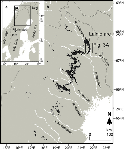
The distribution of the Veiki moraine landscape is significant for discussions of glacial development in Fennoscandia because it is interpreted to mark the easternmost limit of a pre–Late Weichselian Fennoscandian ice sheet (Lagerbäck 1988b; C. Hättestrand 1998; Kleman et al. 2021). Detailed mapping of the Veiki moraine distribution (C. Hättestrand 1998) has shown that the main occurrence is along two parallel elongated zones from River Lainioälven in the north to River Piteälven in the south (Figure 1B). The two zones, separated by 15 to 25 km, consist of three to four well-defined lobes that generally follow the main river valleys. The easternmost part of the distribution is commonly marked by terminal moraines (C. Hättestrand 1998). Lagerbäck (1988b) suggested that Veiki moraine was formed by downwasting of debris-covered regionally stagnant ice, possibly following large-scale surging. C. Hättestrand (1998) proposed that the landscape likely was formed during two major re-advances of an ice sheet, due to the distinct pattern of the two separate lobe systems. In the northern parts of the distribution area, some less obvious marginal positions are also seen, which indicates that more than two re-advances, or stillstands, did occur (C. Hättestrand 1998).

Figure 1. A. Location of map in B and of three interstadial sites mentioned in the text. B. Map showing the distribution of Veiki moraine (in black, from C. Hättestrand 1998) and the study area location in the northernmost lobe (the Lainio arc). © EuroGeographics for the administrative boundaries and the CIA World Data Bank II (WDBII) for rivers.

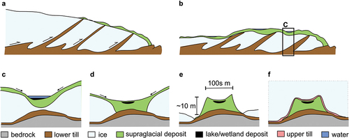
Lagerbäck’s (1988b) general description of the development of Veiki moraine plateaus is today commonly accepted: melting of a debris-covered ice sheet leading to water-filled depressions (ice-walled lakes) that gradually filled up with sediments (i.e., lake deposits), leading to the formation of inversed landforms as the ice melted (Figure 2). The landforms are thus a form of ice-walled lake plains (Clayton et al. 2008). However, what makes the Veiki moraine plateaus distinct from other landforms interpreted as ice-walled lake plains is that they show morphological and stratigraphical evidence of overriding ice, such as weak drumlinization, thin till cover, or scattered glacially transported boulders (Hoppe 1952; Lagerbäck 1988b). These observations led to early interpretations that the plateaus must have been formed subglacially in connection to the last deglaciation (Hoppe 1952, 1957). When Lagerbäck (1988b) instead suggested formation during downwasting of stagnant ice during deglaciation of a pre–Late Weichselian ice sheet, he introduced the concept of marked landforms surviving entire glaciations due to frozen-bed conditions. This led to a completely new view on the glacial history of northern Fennoscandia with a palimpsest landform record of multiple glaciations. Even relatively delicate features such as the rim ridges of the Veiki moraine could be preserved despite being overridden by one or more ice sheets, which, because they were cold-based, had little effect on their substrate (J. Lundqvist and Robertsson 2002; Kleman, Stroeven, and Lundqvist 2008).

Figure 2. Principle sketch of Veiki moraine formation, modified from Sigfúsdóttir (2013). NB. The profiles are vertically exaggerated. (A) Subglacial thrusting in an active ice sheet brings material to the ice surface and creates a thrust moraine at the margin. (B) As the ice stagnates, debris accumulates on the ice surface and a hummocky landscape develops. (C) Supraglacial sand and diamictons are flowing into basins in the ice where fine-grained lake sediment and organic wetland deposits also formed in some cases. (D) As the ice melts, mass movements bring more material into the basin, covering the lake sediments. (E) The ice melts and the former basin turns into a topographic high (a plateau) in the terrain. (F) The plateau is overridden by cold-based ice, which remolds it slightly and leaves a thin till layer on top.

The age of the Veiki moraine is, however, still debated. Lagerbäck (1988b) presented twenty-eight radiocarbon ages from six Veiki moraine plateaus, of which sixteen ages were infinite, older than 35 ¹⁴C ka BP, and twelve were finite, ranging between 39 and 8 ¹⁴C ka BP. However, the radiocarbon dates were regarded as unreliable because there were several cases of reversed ages and some occurrence of ages very close to the Last Glacial Maximum, when the area must have been ice covered. The nonfinite ages were therefore interpreted as being contaminated with recent carbon (Lagerbäck 1988b). Due to the dating problems, Lagerbäck used geographic relations of landforms and lithostratigraphical evidence to infer an age of the Veiki moraine formation. He suggested that the Veiki moraine landscape was formed during deglaciation of the first Weichselian ice sheet in Sweden, during the MIS 5c interstadial (105–93 ka; Lagerbäck 1988b; Lagerbäck and Robertsson 1988). He stated that the Veiki hummocks were related to the northwestern landscape of the pre–Late Weichselian eskers “as many of these eskers enter and integrate with the hummocky moraine terrain” (Lagerbäck 1988b, 479).

Lagerbäck (1988b) also made an attempt to assess how long the formation of the Veiki plateaus within the Lainio arc could have taken. The sediments within the Veiki moraine plateaus differ between sites, where some appear to be built up mainly by diamictons, whereas others contain thick beds of laminated fine-grained water-lain sediments. By approximating the number of lamina (varying between 300 and 2,000) and assuming that the laminae are annual, Lagerbäck estimated that the plateaus could have formed in 300 to 2,000 years.

Based on evidence from detailed geomorphological mapping, C. Hättestrand (1998) later modified Lagerbäck’s contextual interpretation and argued that the Veiki moraine was formed by an ice sheet with a different configuration than the features of the NW landscape, partly since ice flow directions of the Veiki landscape and the NW landscape did not entirely align. The conclusion presented by C. Hättestrand was that the formation of the Veiki moraine and the NW landscape must have been separated in time, even though they both could have been formed during the Early Weichselian, as proposed by Lagerbäck (1988b). Noted by C. Hättestrand (1998) was that the flow direction of the Veiki moraine landscape likely was linked to an ice advance and that many of the northwest-southeast-oriented pre–Late Weichselian eskers disappear when entering the Veiki landscape from the southeast, which could indicate that the eskers were older than the Veiki moraine.

The inferred Early Weichselian age of Veiki moraine formation was later challenged when M. Hättestrand (2007, 2008; Hättestrand and Robertsson, 2010) suggested a younger age, based on biostratigraphical investigations. Pollen records from a kettle hole within the NW landscape were compared with pollen assemblages from a Veiki moraine plateau and both records were thereafter correlated with the more complete Weichselian interstadial record of Sokli, northeast Finland (Figure 1A; Helmens et al. 2000, 2007). It was found that several chronological alternatives of Veiki moraine formation were possible; however, an MIS 3 age was regarded as the most likely (M. Hättestrand 2007, 2008; M. Hättestrand and Robertsson 2010). The interstadial pollen records show evidence of rapid climatic shifts between cold tundra-like conditions and warm phases with climate close to the present, and the Veiki moraine landscape shows signs of glacial surging and periods of stillstands. Climatologically and glaciologically the idea of an intermediate-sized ice sheet being affected by the rapid climatic shifts of MIS 3, as seen in the Greenland ice core records (Rasmussen et al. 2014; Seierstad et al. 2014), would fit well with the geomorphology and stratigraphy of the area. Dating of glacifluvial material and a lateral moraine at Idre and Pilgrimstad, central Sweden (Figure 1A; Alexanderson, Johnsen, and Murray 2010; Möller, Anjar, and Murray 2013; Kleman et al. 2020), have presented evidence of deglaciation of an intermediate-sized ice sheet in Fennoscandia during MIS 3. The margin of such a restricted mountain-centered ice sheet could, according to ice sheet dynamics, reach both Idre and the Veiki moraine area (Kleman et al. 2021). However, there are so far no published ages proving that the ice-marginal features in the two areas are contemporaneous.

In this article, we focus on the chronology of interstadial sediments within the Veiki moraines in northern Sweden (Figure 1) to address the contrasting hypothesis of the age of Veiki moraine formation: Early Weichselian MIS 5c (Lagerbäck 1988b; Lagerbäck and Robertsson 1988) or Middle Weichselian MIS 3 (M. Hättestrand 2007, 2008; M. Hättestrand and Robertsson 2010). We have dated sediments within four Veiki moraine plateaus in the Lainio arc (Rauvospakka, Kortejärvi, Outojärvi, and Sainjärvi; Figure 3) with optically stimulated luminescence (OSL) and radiocarbon, and we use the age of the sediments to discuss the timing of Veiki moraine formation.

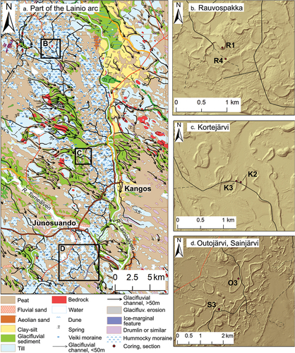
Figure 3. Maps of the field area with details of the four sites. (A) Quaternary deposits map (SGU 2014). See Figure 1 for location within Sweden. (B) Hillshade for Rauvospakka. (C) Hillshade for Kortejärvi. (D) Hillshade for Outojärvi and Sainjärvi. Coring locations (K2, O3, S3), trenches (R1, R2), and road cuts (K3) are marked with red dots. Elevation data in (B)–(D) from Lantmäteriet (2015).

Sites and setting

The study area is located at and north of the confluence of the Lainioälven and Torneälven rivers in northernmost Sweden, close to the Finnish border (Figure 1, Figure 3A). The Paleoproterozoic mainly granitic bedrock is in most places covered by 10 to 20 m of Quaternary deposits dominated by peat, till, and glacifluvial sediment (Figure 3A; SGU 2014, 2016, 2021). Based on previous investigations (Lagerbäck 1988b; Alexanderson, unpubl.; M. Hättestrand, unpubl.) four sites in the Kangos–Junosuando area in Norrbotten were targeted for coring, sedimentological work, and sampling for dating (Kortejärvi, Sainjärvi, Outojärvi, and Rauvospakka; Figure 3, Figure 4, Table S1). These four sites are all Veiki moraine plateaus within the so-called Lainio arc (Figure 1B, Figure 3). Kortejärvi, Sainjärvi, and Outojärvi are characterized by prominent rim ridges surrounding a central low “plateau” with wetlands and/or lakes, whereas the Rauvospakka plateau is higher (Figures 3B–3D; Lagerbäck 1988b; Sigfúsdóttir 2013; Lindqvist 2020).

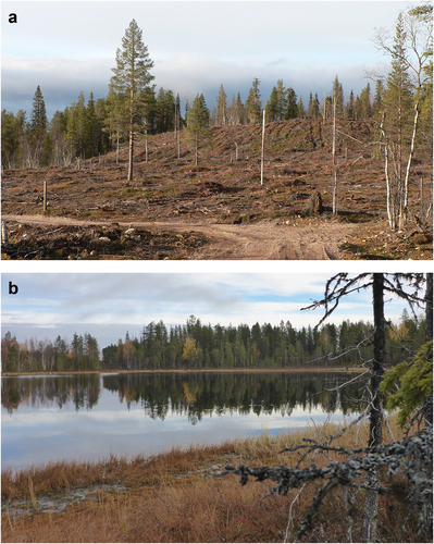
Figure 4. Two Veiki plateaus with different positions in the landscape. (A) The Rauvospakka plateau (photo taken from the south) is relatively high. Sediment infill and peat accumulation occurred at the site during downwasting of an ice sheet; however, after deglaciation the site had no further sediment infill due to its inverted topography (cf. Figure 2, Figure 3b). (B) Sainjärvi, a plateau at low relative elevation (photo taken from the coring point toward the northwest side of the lake and the forested rim ridge). Due to its position in the landscape this site has acted as a sediment trap both during and subsequent to formation of the Veiki plateau; hence, sediment from the supraglacial formation, the following ice-free period, and the Holocene is expected here (cf. Figure 3d). The plateaus at Kortejärvi (Figure 3c) and Outojärvi (Figure 3d) are in this respect similar to Sainjärvi.

The Rauvospakka and Kortejärvi sites have been described by Sigfúsdóttir (2013) and Lindqvist (2020), respectively, and we use some of their data in this article. Outojärvi has previously been studied by Lagerbäck (1988b), but here we present a new core from the same site and also from nearby Sainjärvi.

Methods

Fieldwork and subsampling

Fieldwork was carried out in 2012 (Rauvospakka) and 2018 (Kortejärvi, Outojärvi, Sainjärvi; Table S1). Several trenches, exposures, and cores were documented/taken at each site—hence the numbering of the cores (K2, O3, S3 etc)—but here we only present those from which we have OSL samples. At Rauvospakka, an excavator was used to make trenches ~3 m deep and up to ~18 m long, and small road-cuts (~0.5–1.4 m high) were studied in the rim ridges of the Kortejärvi moraine plateau (site K3), complemented by hand-dug pits to reach deeper. The exposed sediments were described by logging and photo documentation. OSL samples from Rauvospakka and Kortejärvi 3 were taken by hammering opaque plastic tubes into exposed section walls. When the tubes had been fully inserted, they were excavated and the ends were sealed with opaque caps. The samples were stored in light-tight boxes until opened under darkroom conditions. The strategy of sampling was to select samples from different depths within sections of sandy or silty sediments. Samples for determining water content and sediment density were collected in soil sample rings just next to the OSL samples.

The cores from Kortejärvi 2 (K2, 5 m), Outojärvi 3 (O3, 4 m), and Sainjärvi 3 (S3, 3 m) were taken by using a combination of a Russian peat corer (topmost layers consisting of peat) and a cobra vibration corer (Atlas Copco Pionjär) for the lower layers consisting of both peat and minerogenic sediments. The vibration corer was held on hammering mode to be able to penetrate the partly stiff sediments. The cores were collected 1 m at a time in plastic tubes (33-mm diameter), wrapped in dark plastic, and stored in light-tight boxes.

The sample tubes and cores were opened under darkroom conditions. The material from the tubes was separated into subsamples: material from the ends of the tube, which may have seen some light during sampling, was used for measurement of background radiation, and material from the inner part of the tube was used for dose measurements. The cores were split and one of the core halves was sampled for OSL in the darkroom; the other half was used for logging and sampling for radiocarbon dating. The OSL samples were collected from layers with silty to sandy sediments in the cores. Samples for sediment dose rate and water content were collected just below and above each OSL sample.

Samples for ¹⁴C dating were collected from peat layers and from organic material found in the cores. The samples were wet-sieved through a 250-µm sieve with distilled water, dried at 50°C, and sent for accelerator mass spectrometry ¹⁴C dating at the Radiocarbon Dating Laboratory at Lund University. Samples from the depths 67, 138, and 341 cm in the Kortejärvi K2 core were also screened for general pollen composition.

Sample preparation and measurement

Water content was determined by weighing the material in its sampled state (field value), after 24-hour saturation (saturated value) and after 24 hours at 105°C (dry sediment) and calculating the weight of water in relation to the weight of dry sediment.

The sediment used for sediment dose rate determination was dried at 105°C and the samples from Rauvospakka and Kortejärvi were also ashed at 450°C for 24 hours and ground to a fine-grained homogeneous material before being cast into wax of a defined geometry. The contents of U, Th, and K were then measured by high-resolution gamma spectrometry (Murray et al. 1987) at the Nordic Laboratory for Luminescence Dating, Denmark (Rauvospakka, Kortejärvi), and at VKTA–Strahlenschutz, Analytik & Entsorgung Rossendorf e.V., Germany (Outojärvi, Sainjärvi).

The mid-tube material was wet-sieved to extract the 180 – 250-µm fraction, though for the Outojärvi and Sainjärvi samples, wider grain size ranges (e.g. 63–250 µm) had to be used to get enough material for luminescence measurements (Table S2). The fine-sand fraction was then treated with 10 percent hydrochloric acid to remove carbonates and 10 percent H₂O₂ to remove organics. The remaining material was density separated at 2.62 gcm⁻³ (LST Fastfloat) and the heavier, quartz-rich fraction was further treated with 38 to 40 percent hydrofluoric acid for 30 to 60 minutes to etch the grains and 10 percent hydrochloric acid to remove any fluorides. After drying, the material was dry-sieved to remove any material smaller than the finest original fraction (63 or 180 µm).

The dose was measured on the selected quartz mineral fractions as large aliquots in cups (Rauvospakka) and as aliquots on discs (large 8-mm for Kortejärvi and medium 4-mm for Outojärvi and Sainjärvi). Measurements were performed in Risø TL/OSL readers, model DA-20 (Bøtter-Jensen, Thomsen, and Jain 2010), with beta irradiation dose rates of 0.16 to 0.19 Gy/s and blue or post-infrared (IR) blue stimulation at 470 ± 30 nm. Detection was through a 7-mm or 7.5-mm U340 glass filter. The settings of the single aliquot regeneration protocols (Murray and Wintle 2000, 2003; Banerjee et al. 2001; Ankjærgaard et al. 2010) were determined for individual samples by dose recovery and preheat plateau tests (Figure 5) and are listed in Table S2.

Figure 5. Examples of preheat plateau and dose recovery plots. (A) Sample 12057 from Rauvospakka. Both dose recovery ratio and equivalent dose varies with preheat temperature. Preheat at 220°C (cutheat 200°C) was selected for measurement. (B) Sample 20131 from Outojärvi 3. This sample is more stable but shows relatively large spread and the measured dose tends to underestimate the given dose for lower temperatures. Preheat at 260° (cutheat 220°C) was selected for measurement. Three aliquots per temperature were measured; for sample 20131 all aliquots at 240°C had to be rejected because they failed the acceptance criteria.

Dose, dose rate, and age calculation

The dose was calculated by exponential or exponential + linear curve fitting in Risø Analyst (Duller 2008); exponential + linear fitting was used only where a dose could not be calculated with exponential fitting. Early background subtraction was applied for all samples but with different integration limits depending on sample characteristics (Table S2). Aliquots were initially accepted if they had a recycling ratio ≤10 percent and test dose error ≤10 percent. For five samples (Table S2) the limits were increased to 15 percent to get enough aliquots due to high rejection; however, this did not affect the mean dose value. For samples where the dose showed a dependence on apparent feldspar contamination, an additional rejection criterion based on IR/blue ratio was used (Table S2). Aliquots close to or at saturation (D_e > 2D₀) were not rejected on that cause alone (Lowick et al. 2015) but single high-dose outliers were discarded. The fast ratio (FR; Durcan and Duller 2011) was calculated to assess the strength of the fast signal component on a sample basis and was applied as an aliquot rejection criterion only on samples that had more than two aliquots with FR >15.

The ages were calculated based on the mean dose and, following the decision protocol of Arnold, Bailey, and Tucker (2007), on either the central age model (CAM) or the minimum age model with three parameters (MAM3; Galbraith et al. 1999; Burow 2021a, 2021b). The models were applied to the dose data by using the RLuminescence package calc_CentralDose function v1.4.0 (Burow 2021a) and the calc_MinDose function v0.4.4 (Burow 2021b), respectively. The overdispersion of the dose recovery data per site was used as an estimate of sigmab. For samples where the dose distribution statistics imply the MAM3 should be used but the resulting p value is <0.05 the CAM age was used instead.

The total environmental dose rate and final age were calculated using DRAC online (Durcan, King, and Duller 2015). The sediment gamma dose rate for samples taken close to boundaries between two lithologically different units (19003, 20127, 20128, 20138, 20139) was calculated according to Aitken (1985, appendix H), and the beta dose rate was assumed to come from within the sampled layer. The surroundings were considered homogeneous radiation-wise for the remaining samples.

For water content, the saturated value was considered to be a maximum value for the average water content since time of deposition, whereas the field value reflects current conditions. Based on the setting (topography, depth, grain size) of the samples and the landscape development, we estimate the average water content since deposition to be within this range. In the age calculations we therefore used values close to saturation (Table S2) for samples situated in present-day basins (Kortejärvi 2, Outojärvi, Sainjärvi), assuming that these low-lying areas have been lakes or wetlands most of the time since deposition, although while subglacial they likely were in a permafrozen saturated state. For the more elevated samples (Kortejärvi 3, Rauvospakka), the water content was assumed to have been saturated half of the time and equal to present-day field water content the rest of the time (Table S2).

Calibration of radiocarbon ages was done in OxCal v4.4.4 (Bronk Ramsey 2009) using IntCal20 (Reimer et al. 2020). Modern-aged samples were calibrated using the Bomb13 NH1 calibration curve (Hua, Barbetti, and Rakowski 2013; Reimer et al. 2020).

Results

Lithostratigraphic description

The studied sediments are shown in Figures 6 to 8 and summarized below. Additional stratigraphic and sedimentological descriptions and interpretations of the Kortejärvi and Rauvospakka sites are found in Lindqvist (2020) and Sigfúsdóttir (2013), respectively.

Figure 6. Sediment photos. (A) Silty sandy sediments at 2.9 m depth in the Outojärvi core. (B) Gravelly sand at 2.35 to 2.45 cm depth in the Kortejärvi 2 core. (C) Rim ridge sediments at Kortejärvi 3 (Lindqvist 2020, site K3A). (D) Peat and sandy–silty laminated sediments overlain by ~3-m diamicton in Rauvospakka trench 1.

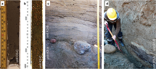
Figure 7. Stratigraphic logs from Outojärvi and Sainjärvi. (A) Outojärvi 3 core. (B) Sainjärvi 3 core. Both mean and modeled OSL ages are shown (most modeled ages are CAM ages, MAM ages are marked with *; Table 2). For further information about the radiocarbon ages, see Table S4. Please note that only the last three digits of the OSL sample number are given here. Ages in gray are considered unreliable based on, for OSL ages, poor luminescence characteristics or incomplete bleaching (poor or bad quality; see Table S2), and for ¹⁴C ages, contamination by younger organic material that was pushed down during coring; see further explanation in text.

Figure 8. Stratigraphic logs. (A) Kortejärvi 2 core. Redrawn from Lindqvist (2020). (B) Composite log from road cuts at Kortejärvi 3 (based mainly on K3A). Samples marked with ^# are taken from the same unit but in other exposures; see Table S2 or details in Lindqvist (2020). Redrawn from Lindqvist (2020). (C) Composite log from Rauvospakka trench 1. Drawn after Sigfúsdóttir (2013). (D) Composite log from Rauvospakka trench 4. Drawn after Sigfúsdóttir (2013). For legend, see Figure 7. Both mean and modeled OSL ages are shown (most modeled ages are CAM ages; MAM ages are marked with *; Table 2). For further information about the radiocarbon ages, see Table S4. Please note that only the last three digits of the OSL sample number are given here. Ages in gray are considered unreliable based on, for OSL ages, poor luminescence characteristics or incomplete bleaching (poor or bad quality, see Table S2) and, for ¹⁴C ages, contamination by younger organic material that was pushed down during coring; see further explanation in text.

Seven lithologic units were distinguished in the Outojärvi core (O3; Figure 7A), which was retrieved from the central basin of a moraine plateau (Figure 3D). The stratigraphy has a slight fining-upwards trend from a sandy diamicton (unit O3-A) at the base through massive gravelly sand (unit O3-B) to massive (unit O3-C; Figure 6A, Figure 7A) and laminated (unit O3-D) sandy–silty sediments. Unit O3-C also contains thin (~5 cm) beds of peat and organic-rich silt. A coarser sediment (unit O3-E gravelly sand) breaks the trend, and the overlying sandy unit O3-F is rich in organic matter. The uppermost unit (O3-G peat) was not studied in detail here.

The 1 m of sediment retrieved from 2- to 3-m depth at Sainjärvi (core S3) contains four lithologic units: two thin minerogenic units at the base (unit S3-A gravelly sand and S3-B sandy silt) overlain by 8 cm gyttja (unit S3-C) and >0.5 m peat (unit S3-D; Figure 7B). A parallel Russian core shows that the peat continues to the present-day surface (total thickness 2.8 m) and is the uppermost unit at the site, which is in the low-lying center of a moraine plateau (Figure 3D).

In the core Kortejärvi K2, from the central part of a low-lying plateau (Figure 3C), four lithologic units were identified: two thin diamictons at the base (units K2-A and -B) overlain by an almost 4-m-thick unit with repeated beds of normally graded gravelly sand (unit K2-C; Figure 6B, Figure 8A). Two thin (~5 cm) beds of peat/organic-rich sediments occur within this unit. The topmost unit is peat (unit K2-D).

At the rim ridge site, Kortejärvi K3 (Figure 3C), two lithologic units were observed. A massive, matrix-supported diamicton (unit K3-A) is overlain by laminated and ripple-laminated sand (unit K3-B; Figure 6C, Figure 8B). In some places thin beds of massive gravelly sand occur within the sand. A few steep faults with mainly centimeter-scale displacement were observed.

At Rauvospakka 1, an approximately 4-m-deep and 18-m-long trench just inside the margin of an elevated plateau (Figure 3B, Figure 4A) revealed massive and laminated sandy silt interbedded with a compacted peat (unit R1-A) at ~3.5-m depth (Figure 6D, Figure 8C). This unit could be traced sub-horizontally along the entire section, although only parts of it could be described in detail due to instability of the section walls. The beds within the unit are wavy and discontinuous and exhibit small-scale flame structures along the upper boundary. The deformation appears to be mostly confined within the unit and to not affect the overlying units. These beds are overlain by two units, both consisting of matrix-supported silty sandy diamicton: unit R1-B (weakly stratified) and unit R1-C (massive).

The Rauvospakka 4 trench cuts into the outer part of a rim ridge of a moraine plateau (Figure 3B). Clast-supported angular boulders (weathered bedrock) were encountered at the base of the trench (unit R4-A, Figure 8D). A sandy diamicton (unit R4-B) with frequent sand and gravel lenses, some of which are folded, lies on top of the bedrock and is in turn overlain by a partly stratified silty sandy diamicton (unit R4-C) and a massive silty sandy diamicton (unit R4-D; Figure 8D).

Sedimentological interpretation

Sedimentologically, seven lithofacies associations (LFA1–7) have been identified in the cores and the exposures (Table 1), the weathered bedrock not included. LFA1 (sandy diamicton) is only found at one site (Rauvospakka 4) and is interpreted as part of the subglacial till that surrounds and likely underlies or forms the lowest part of the Veiki moraine plateaus (Sigfúsdóttir 2013). LFA2 (silty–sandy diamicton) is found at Rauvospakka and is there the topmost unit, forming part of the till cover that drapes the Veiki moraine plateaus (Lagerbäck 1988b; Sigfúsdóttir 2013).

Table 1. Lithofacies associations at the four sites. See Figure 7 for legend.

Lithofacies association	Major lithofacies	Minor lithofacies	Units	Interpretation
LFA1	D(S)m		R4-B	Subglacial traction till
LFA2	D(SiS)mm		R1-C, R4-D	Melt-out till
LFA3	D(SiS)m, D(SiS)ms, GSm	D(S)m, D(G)m, D(Si)m	O3-A, K2-A, -B, K3-A, R1-B, R4-C	Debris flows
LFA4	GSm(ng)	GSm(ig)	O3-B, -E, S3-A, K2-C, K3-B	(Glaci)fluvial deposits (higher energy)
LFA5	Sl, Sr, Sm	Sm(o)	K3-B, O3-F (K2-C)	(Glaci)fluvial deposits (lower energy)
LFA6	SSim, SSil	SSil, Sim, SiSm	O3-C, -D, S3-B, R1-A	(Glaci)lacustrine deposits
LFA7	P	Gy	O3-G, S3-C, -D, K2-D (O3-C, R1-A)	Wetland deposits

LFA3 (variable diamictons and massive gravelly sand) occurs at most sites in low or intermediate stratigraphic positions in or close to rim ridges. These diamictons are interpreted as partly supraglacial debris flows; that is, gravity-driven reworking of material from the surrounding ice surface into the basins that would later form the Veiki moraine plateaus (Sigfúsdóttir 2013; Lindqvist 2020).

LFA4 (gravelly sand) and LFA5 (sand) occur partly interchangeably and are found at all sites except Rauvospakka. The sediments are interpreted to be deposited by flowing water, most likely in subaerial fluvial or glacifluvial streams, and contribute to both the rim ridges and the basin infill in Veiki moraine plateaus (Lindqvist 2020). LFA6 (sandy silt) makes up the most of the Outojärvi core but it is less extensive at the other sites. The beds were deposited in lakes that existed in the central parts of the Veiki moraine plateaus (Lagerbäck 1988b; Sigfúsdóttir 2013; Lindqvist 2020).

The organic LFA7 occurs mainly in surficial position where it is laterally extensive, and thin (5–20 cm) beds occur also in lower stratigraphic positions. The peat at Rauvospakka (unit R1-A) is, in contrast to all other peat beds observed in this study, very compacted (Sigfúsdóttir 2013; M. Hättestrand et al. unpubl.). Although the unit at Rauvospakka containing the peat (R1-A, Figure 8C) is deformed, the peat is interpreted to have been found in its original position or only after very short transport (meters). That conclusion is based on the sub-horizontal, laterally continuous configuration of the unit. The deformation is thus believed to have occurred locally, possibly due to melting of surrounding ice and/or minor disturbance during following deposition. The organic deposits are thus believed to have formed in wetlands in the central parts of the Veiki moraine plateaus, in accordance with the findings of Lagerbäck (1988b). It should be noted that of the nonsurficial organic beds investigated in this study, the peat at Rauvospakka 1 is the only one that is considered to be in situ (see Discussion).

OSL dating

Overall, the luminescence signal from these samples is not very bright; that is, the luminescence signal is not very strong (Figure 9). Only four samples (19004–05, 20127, 20129) have signals with >300 counts/Gy·s (Table S2), which is still lower than the limit for “poor quartz” suggested by Alexanderson (2022). The FR is also relatively low (<10) for most aliquots from most samples, showing that the fast signal component is weak (Figure 9; Durcan and Duller 2011). Exceptions are the upper samples from Outojärvi (20127–20131) and Rauvospakka (12056–57), for which many or most aliquots have FR > 15 or even >20 (Table S2). Additionally, the quartz in approximately two-thirds of the samples showed significant apparent feldspar contamination (IR/B ratio >10 percent) but only three samples showed a dose dependence on the IR/B ratio (Table S2). Of all measured aliquots, 44 percent were rejected based on the criteria described in the Methods. If FR is also used as an aliquot rejection criterion, 87 percent are rejected.

Figure 9. Examples of decay and growth curves. (A) Sample 20129 from Outojärvi 3 has a relatively strong signal dominated by a fast component (fast ratio FR = 31 for this aliquot) that contributes 68 percent of the initial signal. The signal continues to grow to high doses. (B) Sample 20138 from Sainjärvi 3 has a dim signal that has a weaker fast component (53 percent of the initial signal, FR = 6). Both samples have a relatively high background (slow signal component).

The mean equivalent doses range from 27 to 415 Gy (Table 2). Generally, equivalent doses up to ~200 Gy could be measured without reaching saturation (Figure 9). Almost all samples had a few aliquots that were close to or at saturation, but samples with high mean equivalent doses (e.g., 20135, 20137) had several aliquots with D_e > 2D₀. The dose distributions are broad and overdispersed for most samples, with an average relative standard error of the dose of 11 percent and mean overdispersion of 48 percent (Figure 10; Table S2). The most precise and least overdispersed sample is 20139 from Sainjärvi 3 (relative standard error, RSE_De 4 percent, overdispersion 15 percent). All dose distributions except for four samples (18030, 18031, 19006, 20139) are also significantly positively skewed (Figure 10; Table S2).

Table 2. Sample information and luminescence data, sorted by lab number (this is also in stratigraphic order for all sites but Kortejärvi 3, which is a composite site). See Figure 7 and Figure 8 for context and Table S2 for additional luminescence data; for example, overdispersion values and basis for age reliability assessment.

Lab. no Lund	Site or core	Depth (m)	Phase^a	Mean dose (Gy)	n^b	Dose rate (Gy/ka)	Water content (%)	Age reliability	Mean age^c (ka)	Modeled age (ka)	Model^d
12056	Rauvospakka 1	2.7	3	131±16	7/20/45	2.971±0.123	16	Acceptable	47±8	39±5	CAM*
12057	Rauvospakka 1	2.9	3	155±14	5/22/45	3.010±0.125	15	Good	49±7	31±4	MAM3
12058	Rauvospakka 4	2.0	1	176±18	0/17/45	3.191±0.122	17	Bad	55±6	52±6	CAM*
18029	Kortejärvi 3	0.75	2	122±15	1/21/57	2.881±0.110	18	Bad	42±5	37±5	CAM*
18030	Kortejärvi 3	0.48	2	203±21	0/13/48	3.019±0.175	17	Poor	67±8	61±9	CAM*
18031	Kortejärvi 3	1.25	2	140±16	0/14/33	2.892±0.093	19	Poor	49±6	24±3	MAM3
18032	Kortejärvi 3	0.55	2	74.8±9.8	1/15/63	1.615±0.054	19	Poor	46±6	41±6	CAM*
19003	Kortejärvi 2	0.74	7	199±25	1/15/26	2.572±0.170	44	Bad	78±11	71±11	CAM*
19004	Kortejärvi 2	1.58	7	35.9±3.6	4/28/45	2.985±0.241	41	Poor	8.8±1.3	6.2±0.6	MAM3
19005	Kortejärvi 2	2.38	7	41.7±5.8	3/18/45	3.053±0.090	32	Poor	6.4±0.4	6.3±0.5	MAM3
19006	Kortejärvi 2	3.43	7	78.4±9.2	2/17/40	3.112±0.095	27	Acceptable	12±2	9.8±0.9	MAM3
19007	Kortejärvi 2	4.38	7	88±15	1/14/44	3.112±0.096	29	Poor	28±5	23±4	CAM*
20127	Outojärvi 3	1.56	5	71±11	14/14/18	2.364±0.152	19	Acceptable	30±5	25±4	CAM*
20128	Outojärvi 3	1.62	5	71.8±7.5	18/29/42	2.356±0.137	17	Good	32±5	26±3	CAM*
20129	Outojärvi 3	1.71	5	97±10	27/34/39	2.436±0.127	23	Good	43±5	34±4	CAM*
20130	Outojärvi 3	1.92	5	87.0±9.8	19/30/39	2.320±0.119	23	Good	35±6	31±4	CAM*
20131	Outojärvi 3	2.18	5	68.0±7.0	34/40/63	2.049±0.096	58	Good	33±4	26±3	CAM*
20132	Outojärvi 3	2.43	5	92±13	0/30/39	2.575±0.136	26	Poor	36±5	28±4	CAM*
20133	Outojärvi 3	2.92	5	97±11	0/31/36	2.307±0.116	21	Acceptable	42±5	35±4	CAM*
20134	Outojärvi 3	3.28	5	102±16	0/30/48	2.181±0.113	26	Acceptable	47±8	35±5	CAM*
20135	Outojärvi 3	3.50	4	236±17	0/29/30	2.483±0.125	25	Poor	95±9	89±8	CAM*
20136	Outojärvi 3	3.73	4	294±23	3/29/36	2.480±0.125	25	Poor	106±21	72±9	MAM3
20137	Outojärvi 3	3.94	4	415±42	0/26/51	2.479±0.125	25	Bad	167±19	147±18	CAM*
20138	Sainjärvi 3	2.89	7	27.1±1.8	0/35/36	1.900±0.110	56	Good	14.3±1.3	13.5±1.0	CAM*
20139	Sainjärvi 3	2.96	4	86.5±3.7	0/25/41	2.430±0.146	25	Acceptable	36±3	35±3	CAM

Notes. ^aSee Discussion and Figure 11.

^bNumber of accepted aliquots with fast ratio >15, accepted aliquots, and the total number of measured aliquots.

^cAges in bold are based on accepted aliquots that also have a fast ratio >15 (if n > 2); other ages are based on all otherwise accepted aliquots.

^dThe ages have been calculated using the central age model (CAM; Galbraith et al. 1999; Burow 2021a) or the minimum age model with three parameters (MAM3; Galbraith et al. 1999; Burow 2021b). For samples where the dose distribution statistics imply that the MAM3 should be used but the resulting p value is <0.05 (Table S2) the CAM age has been used instead (marked CAM*).

Figure 10. Dose distributions shown as probability plots. (A) Sample 20139 from Sainjärvi 3 has a broad but not significantly skewed dose distribution. (B) Sample 19007 from Kortejärvi 2 has a significantly positively skewed dose distribution. Note that aliquots that lack error bars are those for which Analyst software could not calculate an error due to the dose being at or close to saturation. Both samples were measured as 4-mm aliquots.

Total environmental dose rates range from ~1.6 to 3.2 Gy/ka (Table 2; Table S3). Whether the mean or the central age model is used, most ages fall in the range ~30 to 50 ka (quartiles 1–3; Table 2; Table S2). For about half of the samples, the mean and CAM age overlap within one sigma, whereas the MAM3 ages are lower and not within two sigma of either the corresponding mean or CAM age. However, most of the MAM3 ages are considered unreliable (p < 0.05). For those samples that had some aliquots with FR > 15, ages calculated only based on those aliquots overlap within one sigma with the mean age based on all accepted aliquots; exceptions are those three samples for which there were fewer than five such aliquots (Table S2). However, for these samples the ages overlapped with the corresponding CAM or MAM3 age. At Outojärvi, significantly older ages (>70 ka) are found in the lowest beds (at 3.50–3.94 m), which are characterized by coarser material than the overlying layers of mainly silt and sand (Figure 7A). At Kortejärvi 2 most ages are younger than 30 ka (Figure 8A). OSL ages are generally in stratigraphic order within 2σ at the sites, though there are exceptions at Kortejärvi 2 and 3 (Figures 8A, 8B).

Radiocarbon dating and pollen composition

Fifteen samples of macrofossils and bulk material were dated by accelerator mass spectrometry radiocarbon; of those, fourteen gave Holocene to modern ages (Figure 7, Figure 8, Table S4). A sample of wood (Betula or Alnus) from the compacted peat at Rauvospakka gave an infinite age (>48 ¹⁴C ka BP, >51 cal. ka BP; Figure 8D; Table S4). The ages from the lower part of the uppermost organic units (peat) at both Outojärvi and Sainjärvi range between 9.1 and 5.6 cal. ka BP (Figure 7). At Outojärvi there are age inversions, with young—even modern—ages deeper in the core (Figure 7A) and all ¹⁴C ages from Kortejärvi appear modern (Figure 8A). All pollen samples from Kortejärvi 2 had high percentages of Pinus and Picea.

Discussion

Age reliability assessment

From a luminescence methodological perspective, the most precise and reliable OSL ages come from homogeneous sediments with good luminescence characteristics (strong signal dominated by a fast component) deposited under conditions with effective bleaching and that were analyzed with suitable protocols and with enough data points (Rodnight 2008; Rhodes 2011; Alexanderson 2022). Many of the sampled sediments in this study do not satisfy all of these prerequisites, and a discussion of the reliability of the ages is necessary for evaluation of the chronology of Veiki moraine formation.

Quartz from the study area is fairly dim (brightness range 16–640 counts/Gy∙s), which is on the low side for quartz from Scandinavia (Alexanderson 2022). That the quartz is dim commonly means that it is difficult to measure low doses (young samples), which is not a problem in this study, and that results may be less precise. The OSL dose determinations indeed have fairly low precision (11 percent average relative standard error of the dose; Table S2) compared to those from other Scandinavian quartz (~4 percent, Alexanderson 2022). The dim luminescence signals (Figure 9) also made it necessary to use large or medium aliquots, which unfortunately prevents detailed analysis of dose distributions due to averaging among the many grains (Duller 2008). Additionally, a small amount of material and long measurement times (high doses, high rejection rate) led to low numbers of aliquots, which further limited the application of statistical age models, which preferably should be based on at least fifty D_e values (Rodnight 2008).

Adding a weak fast component to the dim signals, as indicated by the low fast ratio (<10) for many of the samples (Table S2; cf. Durcan and Duller 2011), could mean that the results may also be less accurate because the luminescence signal used for dating is dominated by slower components that may be both harder to bleach and more unstable than a fast component (Steffen, Preusser, and Schlunegger 2009). However, the accuracy of these samples is technically supported by good dose recovery ratios (average 0.99; Table S2) and by getting acceptable results of the built-in quality tests such as recycling ratio, as well as by their overall agreement with those samples that do have high fast ratios indicative of luminescence signals dominated by a fast component. From a geological point of view, the stratigraphic consistency of most OSL ages at the different sites also lends support to their accuracy, even for some of the technically less reliable ages. This is further discussed in the next section.

In addition to the generally less than ideal luminescence characteristics of the analyzed quartz, the depositional processes of some of the dated sediments lead to a risk of incompletely bleached grains, something that the broad and skewed dose distributions (Figure 10) support. Considering the depositional setting, we regard sediments derived from subglacial transport, debris flows, and rapid deposition from bedload (LFA1–4) to be particularly at risk (Fuchs and Owen 2008).

Given the conditions discussed above and the relative range of values for the different characteristics of this sample set, we argue that the most reliable OSL ages in this study are those that come from samples with the brightest quartz (>100 counts/Gy∙s), the strongest fast signal component (mean FR > 15), narrow and nonskewed dose distributions (RSE_De < 10 percent, insignificant skewness), many (>24) aliquots, and consisting of sediment from LFA5 or 6. In terms of accuracy, the most important criterion is the FR, representing a fast signal component, whereas the other criteria relate more to precision and risk of incomplete bleaching. No sample in this study fulfills all of these criteria, but some fulfill enough of them to be considered reliable. Samples that have a mean FR > 15 and fulfill at least two other criteria are classified as good, whereas samples that fulfill three criteria or have high FR plus one other criterion are classified as acceptable (Table 2; Table S2). Together these age classes provide the ages that we rely on the most for our chronology: 12056–57 from Rauvospakka, 19006 from Kortejärvi 2, 20127–131, -133–134 from Outojärvi 3, and 20138–139 from Sainjärvi 3. The remaining ages, which fulfill only two criteria (poor) or one or no criterion (bad; Table 2; Table S2), are considered unreliable and are only used as supporting indications.

With these limitations in mind, we present two ages per sample: the arithmetic mean age as a conservative approach given the low number of aliquots and a modeled age that is associated with a larger theoretical statistical uncertainty but may be considered more accurate in the geological context. Given that dose distributions (skewness, overdispersion) and sedimentology suggest heterogeneously bleached sediments, the mean is likely to overestimate the true age (Kunz et al. 2013; Medialdea et al. 2014; Zhao et al. 2017) and thus provide a maximum age of deposition. The MAM3, which fits a truncated normal distribution to a skewed dose distribution to pick out the lowest dose population (assumed to be completely bleached; Galbraith et al. 1999), is recommended in these cases (Arnold, Bailey, and Tucker 2007). However, with few aliquots per sample, as in this data set, that extracted population becomes very small and the result unreliable (Rodnight 2008). Only for six samples could the MAM3 be used with some reliability (Table 2) but, even so, we consider the MAM3 ages to give minimum estimates for the time of deposition in most cases (Medialdea et al. 2014; Zhao et al. 2017). The CAM ages, which are similar to weighted means, fall between the mean and the MAM3 ages and are considered closer to the true age, but neither over- nor underestimation can be ruled out given the relatively poor statistics (Rodnight 2008; Kunz et al. 2013; Zhao et al. 2017).

Comparison with the radiocarbon ages is unfortunately of limited use to evaluate the OSL ages. The upper radiocarbon ages at Outojärvi and Sainjärvi (5.64–9.06 cal. ka BP) provide only minimum ages compared to the OSL ages and, as such, are not contradictory. The radiocarbon ages from deeper in the Outojärvi and Kortejärvi cores are, however, problematic. These dates do not agree with the much older OSL ages (Figure 7A, Figure 8A) of the minerogenic sediment in which the thin layers of organics are found. The coring was based on flow-through principles, and we believe a few pieces of overlying peat were pushed down during coring, whereafter they were incorporated in the much older minerogenic sediments. The problem of incomplete flow through does not seem to have affected the minerogenic sediment to the same degree, even if some mixing cannot be excluded. We assume that the minerogenics are more or less unaffected because (1) we can identify lithologically different minerogenic beds in the cores, (2) there is a fining-upwards trend, and (3) the OSL ages get older with depth (Figure 7, Figure 8A).

At the sections (Kortejärvi 3, Rauvospakka), the stratigraphy was well exposed. At Rauvospakka 1, the infinite age (>51 cal. ka BP) of wood from a highly compacted but in situ peat bed is believed to represent a true minimum age of the Weichselian interstadial peat being accumulated during a phase of the Veiki moraine formation. It is in good correlation with mean OSL ages of silt just below and above the peat (sample 12057 below: 49 ± 7 ka; sample 12056 above: 47 ± 8 ka; Figure 8C) and also agrees with the modeled ages considering that the underlying MAM3 age (31 ± 4 ka) is a minimum age. However, at Rauvospakka 1 we had problems with collapsing trench walls, and the modern radiocarbon age from a fresh looking Salix leaf, the only distinguishable organic material found within the silt (Figure 8C; Table S4), is thought to come from surficial material collapsing into the trench.

For additional age control, though on a low-resolution level but relevant considering the young radiocarbon ages from some sites, pollen analysis can be used to assess whether the dated sediments are of pre–Late Weichselian or of Holocene origin. The pollen data from the Riipiharju core (M. Hättestrand and Robertsson 2010), retrieved from a site just east of the Veiki moraine of the Lainio arc, can be used as a reference. The Riipiharju data set contains the most complete pollen record from Weichselian ice-free phases in northern Sweden in combination with a pollen record from the Holocene. The pollen assemblages from the Weichselian ice-free phases lack, or have extremely low percentages of, pollen of pine (Pinus) and spruce (Picea), and birch (Betula) and Artemisia are the dominating taxa. For the Holocene, however, all pollen samples from Riipiharju have high values of Pinus and Picea. Because all samples from organic material at Kortejärvi 2 also had high percentages of Pinus and Picea, it was interpreted that the sediment here must have been deposited during the Holocene, which supports the age results retrieved by the modeled OSL ages (Figure 8A). A full pollen analysis was also made on samples from the peat in the Rauvospakka 1 section in a separate study (M. Hättestrand et al. unpubl). Here the analyzed pollen spectra have low/absent values of Pinus and Picea and high percentages of Betula and Artemisia, which shows that the peat in the Rauvospakka 1 section is of Weichselian age. This result is in accordance with the radiocarbon and OSL ages from the peat and the silty layers in Rauvospakka 1.

Chronology of the Veiki moraine

The dated sediment from the four studied sites within the Veiki moraine landscape have ages ranging from 167 ± 19 ka to 5.64 ± 0.04 cal. ka BP (Figure 7, Figure 8, Table 2; excluding the modern radiocarbon ages). The wide age range can be explained by the sediments coming from various parts of the landscape and being deposited during different times and conditions. In addition, methodological problems, such as, for example, partial bleaching, have likely affected some samples more than others, giving older ages than expected for these samples. To understand the retrieved dates and their meaning for the interpretation of Veiki moraine formation and general Fennoscandian ice age history, the dates have been sorted according to stratigraphical, sedimentological, and geomorphological context into depositional phases as discussed below.

Phase 1 (55 ± 6 to 52 ± 6 ka) is represented by the stratigraphically lowest sample, 12058 from Rauvospakka 4 (Figure 8D), which comes from a sandy lens in till (LFA1; Table 1) that surrounds and most likely continues in under or forms the lowermost part of the Veiki moraine plateaus (Sigfúsdóttir 2013; Figure 11A). The sand would have been bleached prior to the ice re-advance that reached the eastern margin of the Veiki moraine and was then incorporated into basal till; as such, it would represent a maximum age for Veiki moraine formation (Figure 11B). This age fits well with the interpretation of deglaciation of an intermediate-sized Fennoscandian ice sheet at Idre in central Sweden, around 55 ka (Kleman et al. 2020), even though the age from Rauvospakka is unfortunately methodologically unreliable due to poor luminescence characteristics.

Figure 11. (A) Schematic cross-profiles of the studied Veiki moraine plateaus with interpreted sediment architecture. See (B) for legend. The profiles from Rauvospakka and Kortejärvi are based on information from ground penetrating radar, trenches, and coring (Sigfúsdóttir 2013; Lindqvist 2020), whereas the profile from Outojärvi, which is also taken to represent Sainjärvi, is modified from a coring-based profile in Lagerbäck (1988b). The profiles are vertically exaggerated and thin units have been made larger for visibility. (B) OSL mean ages and ¹⁴C ages from the four sites separated into groups based on stratigraphic, sedimentological, and geomorphological context and related to different depositional phases in the Veiki moraine formation and subsequent development (see text for explanation). The gray shading indicates our best estimate of the time of formation as ice-walled basins, 56 to 39 ka. Due to low-precision ages the age span is wide but clearly in MIS 3, not MIS 5c. Ages classified as poor or bad are considered unreliable due to methodological issues; see text and Table S2 for details.

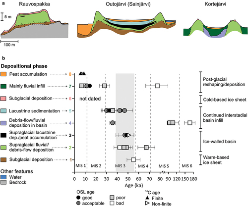
Phase 2 (67 ± 8 to 42 ± 5 ka mean ages; 61 ± 9 to 24 ± 3 ka modeled ages) comprises deposition of coarse sediments (LFA3–5; Table 1) in locations that are topographically high today, such as rim ridges at all sites and the bulk of the plateau at Rauvospakka (Figure 11A). This requires that there were even higher surfaces surrounding these sites to act as sources for the inflowing water and sediment. The easiest explanation for inflow of sediment is that the material came from the debris-covered ice surface surrounding a depression in the ice (Figures 2C, 2D). These deposits must therefore have formed while ice was still present at the site. Thus, the ages of this event, obtained only from Kortejärvi 3 (Figure 8B), represent an early stage of Veiki moraine formation (Sigfúsdóttir 2013; Lindqvist 2020). These OSL ages range from 67 ± 8 (18030 mean age) to 24 ± 3 ka (18031 MAM3 age), though because the latter is considered a minimum age, the range can be reduced to 67 ± 8 to 46 ± 6 ka for mean ages or 61 ± 9 to 41 ± 6 ka for the modeled (CAM) ages (Figure 11). Even so, the ages are partly in reverse stratigraphic order, and all of them are classified as technically poor or bad, which means that the dating of this phase is uncertain.

Phase 3 (49 ± 7 to 47 ± 8 ka mean ages, 39 ± 5 to 31 ± 4 ka modeled ages, >51 cal. ka BP) is represented by fine-grained sediments and organic material (LFA6–7; Table 1) at Rauvospakka 1 (Figure 8C). Following the argumentation for phase 2, sedimentation at the (today) high Rauvospakka plateau requires the presence of a surrounding ice, thus implying supraglacial deposition. The OSL ages are technically good or acceptable (i.e., reliable), and the mean ages, which overlap within errors, agree with the radiocarbon age and are considered the best age determination of this phase (56–39 ka). Of the modeled ages, one is a minimum age (31 ± 4 ka, 12057) and compared to the radiocarbon age (>51 cal. ka BP), the CAM age (39 ± 5 ka, 12056) would also seem to underestimate the true age.

The combined ages of phases 2 and 3 from about 60 ka to 40 ka, best estimate 56–39 ka) would give the timing of the initial stage of Veiki moraine formation, as supraglacial basins at a stagnated former ice margin (Figure 11). However, the full age span (>15 ka) cannot be true, and our interpretation is that the sediments do not represent such a long period of deposition. Compared to other Veiki moraines where (annually) laminated sediments are present, these two phases seems to have lasted at most a few thousand years (Lagerbäck 1988b), a much shorter time span. The 56 to 39 ka age is nevertheless the best that can be achieved given the precision of the data and definitely place the formation of the Veiki moraines and the timing of when the ice margin was at the Lainio arc in the Middle Weichselian, in the early MIS 3. This supports the hypothesis of Hättestrand regarding time of Veiki moraine formation (M. Hättestrand 2007, 2008; M. Hättestrand and Robertsson 2010).

At the same time as the rim ridges formed at the margins of the supraglacial basins—for example, at Kortejärvi 3—deposition must also have taken place in the center of the same basins. However, unlike the high Rauvospakka 1 site, the low topographic level of our other sites (Kortejärvi 2, Outojärvi 3, and Sainjärvi 3), which still at present are characterized by depressions with lakes and wetlands, means that they could also have had sediment infill after the ice sheet had disappeared. Ages from these sites could thus represent the same event as the rim ridges and high plateau samples (i.e., phases 2–3) but could also be related to later stages of sediment infill at the sites, when the ice sheet had lowered significantly or even disappeared (Figure 2). That more than one event is represented by the remaining samples (phases 4–8) is supported by the large age range, c. 150 to 6 ka, and the different type of deposits.

Phase 4 (167 ± 19 to 36 ± 3 ka mean ages, 147 ± 18 to 35 ± 3 ka modeled ages) consists of the oldest group of ages from the low plateaus and comes from gravelly sand and sandy diamicton (LFA3–4; Table 1) at Outojärvi (Figure 7A) and Sainjärvi (Figure 7B). The sediments are interpreted as debris flows or alluvium from the rim ridges toward the center of the depression, as described and illustrated by Lagerbäck (1988b). The sediments could be sourced from the ice surface or be reworked from the rim ridges. The ages occur in stratigraphic order (just within 2 sigma for the modeled ages) but the age variability, skewed dose distributions, and high overdispersion (Table S2), as well as the depositional environment, suggest that these sediments are incompletely bleached and thus that the ages likely are overestimated. The age considered closest to the true depositional age is the 20139 age (36 ± 3 to 35 ± 3 ka; Figure 7B), which also is the only technically reliable age for this phase (Table 2).

Phase 5 (47 ± 8 to 30 ± 5 ka mean ages, 35 ± 5 to 25 ± 4 ka modeled ages, Figure 11B) includes the majority of the ages from Outojärvi 3. The ages are from sandy–silty sediments that in parts are laminated (LFA6; Table 1). We interpret these sediments to represent MIS 3 lacustrine sediment infill, being deposited mainly after formation of the Veiki moraine rim ridges (Figures 2C–2F) at sites in low elevation where sedimentation continued even after the ice was gone. The apparent age span of about 10 to 15 ka found in phase 5 (as exemplified by the Outojärvi core) supports the interpretation of sediment infill during a longer period, though likely the age span is overestimated (cf. discussion for phases 2–3). The youngest modeled ages (25–26 ka; Figure 11B) imply ice-free conditions in our study area when the Fennoscandian ice sheet reached northern Germany (e.g., Hughes et al. 2016). However, the MAM3 ages should be considered minimum ages for the time of deposition and the error margins of the CAM ages, which may over- or underestimate the true age, are relatively large (approximately ±3-5 ka), so if the true ages are on the older side, they would be about 39 to 29 ka. Using mean OSL ages rather than modeled ages would also result in older ages for sediment infill in the plateaus, youngest age is then 30 ± 5 ka (20127 Outojärvi 3). This agrees better with reconstructions of ice sheet expansion leading up to the Last Glacial Maximum (LGM), which show that our study area became ice-covered sometime between 34 and 30 ka (Hughes et al. 2016), which would put an end to lacustrine sedimentation in the Veiki moraine plateaus. All ages but one are considered technically reliable; the exception is 20132, which nevertheless agrees well with the other ages. However, as for previous phases, the low precision of the ages prevents better discrimination of both timing and duration of this depositional event.

Lagerbäck (1988a) identified evidence of past extensive frost-shattering, permafrost, and wind erosion and linked this evidence to Weichselian ice-free phases with harsh climatic conditions. Likely wind-blown sand came into the low elevation Veiki plateaus during these colder phases, though all Weichselian pollen records studied from Veiki plateaus so far (Rissejauratj, Kurujärvi, and Rauvospakka) reveal pollen spectra with high percentages of birch, showing evidence of sediment deposition during relatively warm phases (M. Hättestrand 2007; M. Hättestrand et al. unpubl). The occurrence of windblown material into the Veiki depressions could possibly be supported by the observation that the OSL samples with the highest sensitivity, strongest fast signal component, and least apparent age overestimation are found in the uppermost unit at Outojärvi 3 (depositional phase 5; Table S2). Eolian sediments are generally well suited for luminescence dating (Rhodes 2011), and sensitivity has in other parts of the world has been seen to increase with longer transport distance and more erosion/sedimentation cycles (Pietsch, Olley, and Nanson 2008; Gliganic et al. 2017), something that would be the case for the eolian deposits in this area, which are reworked from mainly glacifluvial deposits (Seppälä 1972). Because both the Outojärvi and the Sainjärvi plateaus are surrounded by clear rim ridges, it is less likely that the inflow of material in these depressions is of fluvial origin, though alluvial and colluvial reworking of rim ridge material most likely contributed to the sediment supply. The rim ridge of the plateau at Kortejärvi is, on the other hand, fragmented (Figure 3C), likely due to fluvial erosion (Lindqvist 2020), and hence it is likely that this plateau could have been destroyed by fluvial action after its initial stage of formation and that flowing water continued to bring in material.

Phase 6 has not been dated by us but is at some of our sites represented by a thin till cover (Rauvospakka; Sigfúsdóttir 2013) or scattered glacially transported boulders (Kortejärvi; Lindqvist 2020; Figure 11A) that were deposited likely during the deglaciation of a cold-based ice sheet. We correlate this phase to the Late Weichselian (LGM).

Phase 7 (28 ± 5 to 6.4 ± 0.4 ka mean ages, 23 ± 4 to 6.2 ± 0.6 ka modeled ages) consists of minerogenic sediments from Kortejärvi 2 and Sainjärvi 3 (Figure 7B, Figure 8A, Figure 11). These sediments represent fluvial or lacustrine deposition (LFA4–5; Table 1). The unreliable and chronostratigraphically inversed sample 19003 (78 ± 11 ka) has been excluded, and three of the other samples are also technically unreliable. One of these, 19007 (28 ± 5 to 23 ± 4 ka) from Kortejärvi and also the good sample 20138 (14 ± 1 ka) from Sainjärvi are unlikely true, given that the area was not deglaciated until ~10.1 to 10.0 cal. ka BP (Stroeven et al. 2016). However, both samples yield MAM3 ages <10 ka (7.8 and 9.4 ka, respectively, Table S2), which shows that there is a small population of aliquots with doses that would yield an age in the expected range, but they are too few to be reliable. The otherwise oldest age in this group (12 ± 2 to 9.8 ± 0.9 ka, 19006 from Kortejärvi; Figure 8A), which is technically acceptable (Table 2), overlaps with the timing of deglaciation, and we believe that these sediments are not linked to the Veiki formation phase sensu stricto. Rather, we interpret that they were deposited during a Holocene phase of erosion and sedimentation at the sites, most likely initiated during the last deglaciation (Lindqvist 2020) but continuing for some time afterward.

Phase 8 (9.06 ± 0.08 to 5.64 ± 0.04 cal. ka BP) consist of radiocarbon ages from organic deposits that form the uppermost stratigraphic units at Outojärvi 3 and Sainjärvi 3 (Figure 7, Figure 11). By correlation, unit K2-D at Kortejärvi may also be included in this group, despite its apparent modern age (Figure 8A). These deposits represent postglacial vegetation establishment and either lake overgrowth (Sainjärvi) or swamping (Outojärvi, Kortejärvi) during the Holocene.

Implications for the glacial history of northern Fennoscandia

Despite the wide span of our retrieved ages for the early phase of Veiki moraine formation (~60–40 ka), the results are a large step forward when studying MIS 3 interstadial conditions in Fennoscandia. Our dates of the Veiki landscape show that it was formed during MIS 3 and not MIS 5c, as suggested in previous studies (Lagerbäck 1988b; Lagerbäck and Robertsson 1988; C. Hättestrand 1998). Evidence of melting of a relatively small, mountain-centered MIS 3 ice sheet, with its easternmost margin in the Veiki area, is in accordance with the evidence of warm ice-free MIS 3 conditions in central Fennoscandia that has been presented earlier through dating of sites with interstadial sediments and fossils (Ukkonen et al. 2007; Alexanderson, Johnsen, and Murray 2010; Wohlfarth 2010; Möller, Anjar, and Murray 2013; Kleman et al. 2020). In addition, compared to most previous studies, our results have the benefit of also pinpointing the exact position of a MIS 3 ice sheet margin. Thus, the formation of Veiki moraine can be linked to both ice sheet extent and climate history.

The Middle Weichselian glacial maximum occurred in MIS 4 and the ice sheet then covered most of Fennoscandia, with its eastern margin close to the eastern border of Finland (Svendsen et al. 2004; Johansson, Lunkka, and Sarala 2011; Batchelor et al. 2019). In a map reconstruction, Svendsen et al. (2004; figure 15) showed the ice sheet extent approximately 60 ka ago; that is, contemporaneous with our maximum age of the Veiki moraine (Figure 11). Because the Veiki moraine was formed by a much smaller ice sheet, it must have been formed later than when the ice sheet had an extent as that presented for 60 ka in Svendsen et al. (2004).

Our further discussion is based on the assumptions that (1) the main phases of waxing and waning of the MIS 3 ice sheet in Fennoscandia are linked to the overall climatic shifts seen in the Greenland ice core record (Rasmussen et al. 2014) and (2) that approximate maximum MIS 3 melting speeds could be estimated through comparison with deglaciation speeds of the Fennoscandian ice sheet during the last deglaciation in the early Holocene. If we further assume that the melting of the large MIS 4 ice sheet that reached eastern Finland about 60 ka started when climatic conditions shifted from the long-lasting cold stadial conditions of Greenland Stadial GS-18 to the warmer conditions of Greenland Interstadial GI-17.2, the deglaciation should have started at approximately 59.4 ka (Rasmussen et al. 2014). During the early part of the Holocene, the deglaciation of the eastern margin of the Fennoscandian ice sheet from easternmost Finland to central northern Sweden took about 1,500 years (Stroeven et al. 2016). The outline of the Veiki landscape as moraine lobes (Figure 1B) shows that there was ice expansion prior to the formation of the Veiki landscape, not just a steady retreat (C. Hättestrand 1998). Hence, after 59.4 ka there must both have been approximately 1,500 years of deglaciation to allow the ice sheet margin to retreat beyond (west of) the Veiki zone and thereafter a sufficiently long period of cold climate to result in an ice advance with ice lobes reaching the Veiki area. After this the Veiki moraine landscape was formed during a phase with warmer climate and slow melting of the debris-covered ice.

The first Greenland Interstadials after 59.4 ka (GI-17.2-GI–16.2) lasted only 140 to 520 years each, so they were likely too short to cause enough deglaciation for the ice sheet margin to retreat from eastern Finland to central Sweden, even though they might have caused partial retreat. GI-16.1 (58.0–56.5 ka), on the other hand, lasted about 1,500 years, a time that could have been long enough to allow for substantial deglaciation, as discussed above in the comparison with the early Holocene ice retreat rates. Hence, it is reasonable to believe the ice sheet margin could have been positioned west of the area of the Veiki landscape toward the end of GI-16.1 (at about 56.5 ka).

The relatively long GI-16.1 was followed by three periods with colder conditions (GS-16.1, GS-15.2, and GS-15.1; 56.5–54.2 ka) that could have caused the ice expansion leading up to Veiki moraine formation. The fact that the Veiki moraine landscape is formed in two parallel zones indicates two subsequent periods of ice advance relatively close in time with a shorter period of melting in between (C. Hättestrand 1998). This fits with the climatic history of the three successive stadials GS-16.1, GS-15.2, and GS-15.1 that lasted about 700, 400, and 680 years, respectively, and the time matches well with our (unreliable) OSL age of depositional phase 1 (subglacial deposition after 55 ± 6 to 52 ± 6 ka; Figure 11B).

After GS-15.1 there is the long GI-14 interstadial, which began 54.2 ka and lasted about 5,880 years (Rasmussen et al. 2014). This stadial likely represents a period of ice melt that is too long to represent a short warm phase in between the two distinct phases of ice advance that formed the two zones of the Veiki landscape. Instead, we find it more likely that this is the time when much of the ice within the Veiki moraine landscape melted off and when ice-walled lakes and mires existed within the debris-covered ice lobes; that is, corresponding to depositional phases 2 to 3 (Figure 11). The precision of the OSL ages is not sufficient to correlate to a specific Greenland Interstadial, even one as long as GS-15.1, but our ages do not contradict the correlation. Due to the insulating debris cover, the melting of the ice leading to eventual topographic inversion of the landscape took a long time, though likely not as long as indicated by the full range of the OSL ages (>15 ka; Figure 11B), as discussed above.

It is probable that a large part, if not all, of the MIS 3 ice sheet eventually melted away during GI-14. A recent compilation of OSL, radiocarbon, and cosmogenic nuclide dating show that central Scandinavia likely was ice free between 55 and ca. 35 ka (Kleman et al. 2021), which would fit with large-scale ice retreat during GI-16.1. Kleman et al. (2021) estimated that the maximum sea-level contribution of a Fennoscandian intermediate-sized ice sheet, an ice sheet with its eastern margins in the Veiki area in the north and at Idre further south, would be less than 1 m. An ice sheet of this configuration during the period of 56.5 and 54.2 ka fits both with the datings at Idre and with our interpretations presented above linking geomorphology and dating of the Veiki moraine landscape to the climatic record of the Greenland ice cores.

Conclusions

Four sites within the Lainio arc of the Veiki moraine belt in northern Sweden were investigated with the purpose to date the time of formation. Previous research has shown that the Veiki moraine landscape, morphologically similar to the ice-walled lake plains in North America, was formed during downwasting of debris-covered ice at the easternmost margin of an intermediate-sized pre-LGM Fennoscandian ice sheet (Lagerbäck 1988b). Preservation of the landscape during the following glaciation has been explained by frozen-bed ice sheet conditions. However, contrasting hypotheses regarding the age of formation have been put forward. We present ages of twenty-five OSL dates and fifteen radiocarbon dates from a range of sediments. The OSL ages have low precision due to poor quartz luminescence characteristics. This prevents detailed statistical analyses of the data, as well as precise comparisons with other records. Nevertheless, the ages clearly place the time of Veiki moraine formation in MIS 3, during the Middle Weichselian, as proposed by M. Hättestrand (2007, 2008; Hättestrand and Robertsson 2010), and not in MIS 5c (Early Weichselian; Lagerbäck 1988b; Lagerbäck and Robertsson 1988).

The plateaus started forming as supraglacial basins (ice-walled lakes/wetlands) in which debris flows and sorted sediments as well as organic deposits accumulated. This took place during a few thousand years sometime between 56 and 39 ka (phases 2–3; Figure 11). As the ice melted away fully, the basins were topographically inverted and became plateaus surrounded by rim ridges. Sedimentation ceased in high plateaus and rim ridges but continued in low-lying plateaus where depressions are still present today. Lacustrine deposition likely continued in these depressions until the Fennoscandian ice sheet expanded over the area, no later than ~30 ka (phase 5; Figure 11). During and following the last (post-LGM) deglaciation at 10.0 to 10.1 cal. ka BP (Stroeven et al. 2016), meltwater caused erosion and reworking of some of the plateaus. Infilling with fluvial sediments and accumulation of peat continued during the Holocene until present in low-lying parts of the Veiki landscape (phases 7–8; Figure 11).

Based on the relation of our data on Veiki moraine formation with geomorphology and other data on ice sheet history and climate variability during MIS 4 and 3 (Greenland ice core records), we suggest that an extensive ice retreat leading to an ice sheet with its margin west of the Veiki moraine zone could have occurred during GI-16.1 (58.0–56.5 ka). Ice sheet advances resulting in debris-covered ice lobes in the Veiki area fit in timing and scale with the relatively short-lived stadials GS-16.1, GS-15.2, and GS-15.1 (56.5–54.2 ka). A final melting of the debris-covered ice, leading to the formation of the Veiki moraine and its ice-walled basins, could then have occurred during the long GI-14, which began 54.2 ka and lasted about 5,880 years.

Acknowledgments

We thank Petra Zahajská (Lund University) and Leif Vidar Jakobsen (Norwegian University of Life Sciences) for field assistance. We also thank Clas Hättestrand for participation in identification of the Rauvospakka field area, early fieldwork performing ground penetrating radar investigations, and fruitful discussions. Editor Chris Stokes and two anonymous reviewers provided constructive comments on the article.

Disclosure statement

The authors have no conflicts of interest to report.

Supplementary material

Supplemental material for this article can be accessed on the publisher’s website.

Additional information

Funding

This work was supported by the Geological Survey of Sweden under Grant 36-2021/2016 and by the Royal Physiographic Society in Lund.

References

- Aartolahti, T. 1974. Ring ridge hummocky moraines in northern Finland. Fennia-International Journal of Geography 134, 22.
- Aitken, M. J. 1985. Thermoluminescence dating, 359. London: Academic.
- Alexanderson, H., and A. S. Murray. 2007. Was southern Sweden ice free at 19-25 ka, or were the post LGM glacifluvial sediments incompletely bleached? Quaternary Geochronology 2 (1–4):229–36. doi:10.1016/j.quageo.2006.05.007.
- Alexanderson, H., T. Johnsen, and A. S. Murray. 2010. Re-dating the Pilgrimstad interstadial with OSL: A warmer climate and a smaller ice sheet during the Swedish Middle Weichselian (MIS 3)? Boreas 39 (2):367–76. doi:10.1111/j.1502-3885.2009.00130.x.
- Alexanderson, H., M. Hättestrand, J. P. Buylaert. 2011. New dates from the Riipiharju interstadial site, northernmost Sweden. Vol. 71 of INQUA PeriBaltic Working Group; Geological Survey of Finland, eds. P. Johansson, J. P. Lunkka, and P. Sarala. Northern Finland: Geological Survey of Finland.
- Alexanderson, H., and A. S. Murray. 2012. Problems and potential of OSL dating Weichselian and Holocene sediments in Sweden. Quaternary Science Reviews 44:37–50. doi:10.1016/j.quascirev.2009.09.020.
- Alexanderson, H. 2022. Luminescence characteristics of Scandinavian quartz, their connection to bedrock provenance and influence on dating results. Quaternary Geochronology 69:101272. doi:10.1016/j.quageo.2022.101272.
- Ankjærgaard, C., M. Jain, K. J. Thomsen, and A. S. Murray. 2010. Optimising the separation of quartz and feldspar optically stimulated luminescence using pulsed excitation. Radiation Measurements 45 (7):778–85. doi:10.1016/j.radmeas.2010.03.004.
- Arnold, L. J., R. M. Bailey, and G. E. Tucker. 2007. Statistical treatment of fluvial dose distributions from southern Colorado arroyo deposits. Quaternary Geochronology 2 (1–4):162–67. doi:10.1016/j.quageo.2006.05.003.
- Banerjee, D., A. S. Murray, L. Bøtter-Jensen, and A. Lang. 2001. Equivalent dose estimation using a single aliquot of polymineral fine grains. Radiation Measurements 33 (1):73–94. doi:10.1016/S1350-4487(00)00101-3.
- Batchelor, C. L., M. Margold, M. Krapp, D. K. Murton, A. S. Dalton, P. L. Gibbard, C. R. Stokes, J. B. Murton, and A. Manica. 2019. The configuration of Northern Hemisphere ice sheets through the Quaternary. Nature Communications 10 (1):3713. doi:10.1038/s41467-019-11601-2.
- Bøtter-Jensen, L., K. J. Thomsen, and M. Jain. 2010. Review of optically stimulated luminescence (OSL) instrumental developments for retrospective dosimetry. Radiation Measurements 45 (3–6):253–57. doi:10.1016/j.radmeas.2009.11.030.
- Bronk Ramsey, C. 2009. Bayesian analysis of radiocarbon dates. Radiocarbon 51 (1):337–60. doi:10.1017/S0033822200033865.
- Burow, C. 2021a. Calc_CentralDose(): Apply the central age model (CAM) after Galbraith et al. (1999) to a given De distribution: Function version 1.4.0. In Luminescence: Comprehensive luminescence dating data analysis. R package version 0.9.11, S. Kreutzer, C. Burow, M. Dietze, M. C. Fuchs, C. Schmidt, M. Fischer, J. Friedrich, N. Mercier, S. Riedesel, and M. Autzen, et al. ed., 1.4.0., Function version https://CRAN.R-project.org/package=Luminescence(accessed December 13, 2021).
- Burow, C. 2021b. Calc_MinDose(): Apply the (un-)logged minimum age model (MAM) after Galbraith et al. (1999) to a given De distribution. Function version 0.4.4. In Luminescence: Comprehensive luminescence dating data analysis. R package version 0.9.11, S. Kreutzer, C. Burow, M. Dietze, M. C. Fuchs, C. Schmidt, M. Fischer, J. Friedrich, N. Mercier, S. Riedesel, M. Autzen, et al. ed.,
- Clark, P. U., A. S. Dyke, J. D. Shakun, A. E. Carlson, J. Clark, B. Wohlfarth, J. X. Mitrovica, S. W. Hostetler, and A. M. McCabe. 2009. The last glacial maximum. Science 325 (5941):710–14. doi:10.1126/science.1172873.
- Clayton, L., J. W. Attig, N. R. Ham, M. D. Johnson, C. E. Jennings, and K. M. Syverson. 2008. Ice-walled-lake plains: Implications for the origin of hummocky glacial topography in middle North America. Geomorphology 97 (1–2):237–48. doi:10.1016/j.geomorph.2007.02.045.
- Daniel, E. 1975. Glacialgeologi inom kartbladet Moskosel i mellersta Lappland. Geological Survey of Sweden Ba 25:121.
- Duller, G. A. T. 2008. Single-grain optical dating of Quaternary sediments: Why aliquot size matters in luminescence dating. Boreas 37 (4):589–612. doi:10.1111/j.1502-3885.2008.00051.x.
- Durcan, J. A., and G. A. T. Duller. 2011. The fast ratio: A rapid measure for testing the dominance of the fast component in the initial OSL signal from quartz. Radiation Measurements 46 (10):1065–72. doi:10.1016/j.radmeas.2011.07.016.
- Durcan, J. A., G. E. King, and G. A. T. Duller. 2015. DRAC: Dose rate and age calculator for trapped charge dating. Quaternary Geochronology 28:54–61. doi:10.1016/j.quageo.2015.03.012.
- Fredholm, K. A. 1886. Öfversigt af Norrbottens geologi inom Pajala, Muonionalusta och Tärändö socknar. Geological Survey of Sweden C 83:39.
- Fuchs, M., and L. A. Owen. 2008. Luminescence dating of glacial and associated sediments: Review, recommendations and future directions. Boreas 37 (4):636–59. doi:10.1111/j.1502-3885.2008.00052.x.
- Galbraith, R. F., R. G. Roberts, G. M. Laslett, H. Yoshida, and J. M. Olley. 1999. Optical dating of single and multiple grains of quartz from Jinmium rock shelter, northern Australia. Part I: Experimental design and statistical models. Archaeometry 41 (2):339–64. doi:10.1111/j.1475-4754.1999.tb00987.x.
- Geijer, P. 1917. Om landisens avsmältningsförhållanden inom Nautanenområdet vid Gällivare. Geological Survey of Sweden C 277. 36.
- Geijer, P. 1948. Några synpunkter på isavsmältningens förlopp i nordligaste Sverige. Geologiska Föreningen i Stockholm Förhandlingar 70 (4):575–82. doi:10.1080/11035894809445153.
- Gliganic, L. A., T. J. Cohen, M. Meyer, and A. Molenaar. 2017. Variations in luminescence properties of quartz and feldspar from modern fluvial sediments in three rivers. Quaternary Geochronology 41:70–82. doi:10.1016/j.quageo.2017.06.005.
- Gravenor, C. P., and W. O. Kupsch. 1959. Ice-disintegration features in western Canada. The Journal of Geology 67 (1):48–64. doi:10.1086/626557.
- Hättestrand, M., H. Alexanderson, T. Sigfúsdóttir, E. Hammarström, C. Hättestrand, M. Regnell, and J. Kleman In prep.: Evidence of decay of an intermediate sized ice sheet during warm climatic conditions in MIS 3 in northern Sweden.
- Hättestrand, C. 1998. The glacial geomorphology of central and northern Sweden. Geological Survey of Sweden Ca 85:47.
- Hättestrand, M. 2007. Weichselian interstadial pollen stratigraphy from a Veiki plateau at Rissejauratj in Norrbotten, northern Sweden. GFF 129 (4):287–94. doi:10.1080/11035890701294287.
- Hättestrand, M. 2008: Vegetation and climate during Weichselian ice free intervals in northern Sweden. Stockholm University, PhD thesis. 35 pp. http://urn.kb.se/resolve?urn=urn:nbn:se:su:diva-8222.
- Hättestrand, M., and A.-M. Robertsson. 2010. Weichselian interstadials at Riipiharju, northern Sweden – Interpretation of vegetation and climate from fossil and modern pollen records. Boreas 39 (2):296–311. doi:10.1111/j.1502-3885.2009.00129.x.
- Hättestrand, C., H. Alexanderson, M. Hättestrand, T. Sigfusdottir, and L. V. Jakobsen 2014: Veiki moraine–morphology, stratigraphy and paleoglaciological implications of an ice-walled lake plain topography in northern Sweden. 31st Nordic Geological Winter Meeting, 2014, Lund, Sweden.
- Helmens, K. F., M. E. Räsänen, P. W. Johansson, H. Jungner, and K. Korjonen. 2000. The last interglacial-glacial cycle in NE Fennoscandia: A nearly continuous record from Sokli (Finnish Lapland). Quaternary Science Reviews 19 (16):1605–23. doi:10.1016/S0277-3791(00)00004-4.
- Helmens, K. F., P. W. Johansson, M. E. Räsänen, H. Alexanderson, and K. O. Eskola. 2007. Ice-free intervals at Sokli continuing into Marine Isotope Stage 3 in the central area of the Scandinavian glaciations. Bulletin of the Geological Society of Finland 79 (1):17–39. doi:10.17741/bgsf/79.1.002.
- Högbom, A. 1931. Praktisk-geologiska undersökningar inom Jokkmokk. Geological Survey of Sweden C 369:57.
- Hoppe, G. 1952. Hummocky moraine regions with special reference to the interior of Norrbotten. Geografiska Annaler 67:48–67.
- Hoppe, G. 1957. Problems of glacial morphology and the Ice Age. Geografiska Annaler 39:1–18.
- Hua, Q., M. Barbetti, and A. Z. Rakowski. 2013. Atmospheric radiocarbon for the period 1950–2010. Radiocarbon 55 (4):2059–72. doi:10.2458/azu_js_rc.v55i2.16177.
- Hughes, A. L. C., R. Gyllencreutz, Ø. S. Lohne, J. Mangerud, and J. I. Svendsen. 2016. The last Eurasian ice sheets – A chronological database and time-slice reconstruction, DATED-1. Boreas 45:1–45.
- Johansson, P., and J. Nenonen. 1991. Till stratigraphical studies in the Pulju area in northern Finland. Geological Survey of Finland, Special Paper 12:131–34.
- Johansson, P., J. P. Lunkka, and P. Sarala. 2011. The glaciation of Finland. In Developments in quaternary sciences, ed. P. L. G. Jürgen Ehlers and D. H. Philip, 105–16. Elsevier.
- Kleman, J., A. P. Stroeven, and J. Lundqvist. 2008. Patterns of Quaternary ice sheet erosion and deposition in Fennoscandia and a theoretical framework for explanation. Geomorphology 97 (1–2):73–90. doi:10.1016/j.geomorph.2007.02.049.
- Kleman, J., M. Hättestrand, I. Borgström, F. Preusser, and D. Fabel. 2020. The Idre marginal moraine – An anchorpoint for middle and late Weichselian ice sheet chronology. Quaternary Science Advances 2:100010. doi:10.1016/j.qsa.2020.100010.
- Kleman, J., M. Hättestrand, I. Borgström, D. Fabel, and F. Preusser. 2021. Age and duration of a MIS 3 interstadial in the Fennoscandian Ice Sheet core area – Implications for ice sheet dynamics. Quaternary Science Reviews 264:107011. doi:10.1016/j.quascirev.2021.107011.
- Knudsen, C. G., E. Larsen, H. P. Sejrup, and K. Stalsberg. 2006. Hummocky moraine landscape on Jæren, SW Norway—implications for glacier dynamics during the last deglaciation. Geomorphology 77 (1–2):153–68. doi:10.1016/j.geomorph.2005.12.011.
- Kujansuu, R. 1967. On the deglaciation of western finnish lapland. Bulletin de la Commission Géologique de Finlande 232:98.
- Kunz, A., D. Pflanz, T. Weniger, B. Urban, F. Krüger, and Y.-G. Chen. 2013. Optically stimulated luminescence dating of young fluvial deposits of the Middle Elbe River Flood Plains using different age models. Geochronometria 41 (1):36–56. doi:10.2478/s13386-013-0140-7.
- Lagerbäck, R., and A.-M. Robertsson. 1988. Kettle holes - stratigraphical archives for Weichselian geology and palaeoenvironment in northernmost Sweden. Boreas 17 (4):439–68. doi:10.1111/j.1502-3885.1988.tb00561.x.
- Lagerbäck, R. 1988a. Periglacial phenomena in the wooded areas of Northern Sweden - relicts from the Tärendö Interstadial. Boreas 17 (4):487–99. doi:10.1111/j.1502-3885.1988.tb00563.x.
- Lagerbäck, R. 1988b. The Veiki moraines in northern Sweden - widespread evidence of an early Weichselian deglaciation. Boreas 17 (4):469–86. doi:10.1111/j.1502-3885.1988.tb00562.x.
- Lagerbäck, R. 2007. Ventifacts – Means to reconstruct glacial development and palaeoenvironment in northern and central Sweden. GFF 129 (4):315–24. doi:10.1080/11035890701294315.
- Lantmäteriet 2015: Product description: GSD-elevation data, grid 2+.
- Lindqvist, M. A. 2020. Kortejärvi Veiki moraine plateau - a key to the glacial history of northern Sweden. UiT the Arctic University of Norway, MSc Thesis 109. https://hdl.handle.net/10037/18227
- Lowick, S. E., M. W. Buechi, D. Gaar, H. R. Graf, and F. Preusser. 2015. Luminescence dating of Middle Pleistocene proglacial deposits from northern Switzerland: Methodological aspects and stratigraphical conclusions. Boreas 44 (3):459–82. doi:10.1111/bor.12114.
- Lundqvist, G. 1943. Norrlands jordarter. Geological Survey of Sweden C 457:166.
- Lundqvist, J. 1981. Moraine morphology: Terminological remarks and regional aspects. Geografiska Annaler: Series A, Physical Geography 63:127–38.
- Lundqvist, J., and A.-M. Robertsson. 2002. Istider och mellanistider. In Sveriges Nationalatlas: Berg och jord, C. Fredén ed., 3rd ed., 120–24.
- Medialdea, A., K. J. Thomsen, A. S. Murray, and G. Benito. 2014. Reliability of equivalent-dose determination and age-models in the OSL dating of historical and modern palaeoflood sediments. Quaternary Geochronology 22:11–24. doi:10.1016/j.quageo.2014.01.004.
- Minell, H. 1979. The genesis of tills in different moraine types and the deglaciation in a part of central Lapland. Geological Survey of Sweden Ca 754:83.
- Möller, P., J. Anjar, and A. S. Murray. 2013. An OSL-dated sediment sequence at Idre, west-central Sweden, indicates ice-free conditions in MIS 3. Boreas 42 (1):25–42. doi:10.1111/j.1502-3885.2012.00284.x.
- Murray, A. S., R. Marten, A. Johnson, and P. Martin. 1987. Analysis for naturally occurring radionuclides at environmental concentrations by gamma spectrometry. Journal of Radioanalytical and Nuclear Chemistry Articles 115 (2):263–88. doi:10.1007/BF02037443.
- Murray, A. S., and A. G. Wintle. 2000. Luminescence dating of quartz using an improved single-aliquot regenerative-dose protocol. Radiation Measurements 32 (1):57–73. doi:10.1016/S1350-4487(99)00253-X.
- Murray, A. S., and A. G. Wintle. 2003. The single aliquot regenerative dose protocol: Potential for improvements in reliability. Radiation Measurements 37 (4–5):377–81. doi:10.1016/S1350-4487(03)00053-2.
- Pietsch, T. J., J. M. Olley, and G. C. Nanson. 2008. Fluvial transport as a natural luminescence sensitiser of quartz. Quaternary Geochronology 3 (4):365–76. doi:10.1016/j.quageo.2007.12.005.
- Rasmussen, S. O., M. Bigler, S. P. Blockley, T. Blunier, S. L. Buchardt, H. B. Clausen, I. Cvijanovic, D. Dahl-Jensen, S. J. Johnsen, H. Fischer, et al. 2014. A stratigraphic framework for abrupt climatic changes during the Last Glacial period based on three synchronized Greenland ice-core records: Refining and extending the INTIMATE event stratigraphy. Quaternary Science Reviews 106:14–28. doi:10.1016/j.quascirev.2014.09.007.
- Reimer, P. J., W. E. Austin, E. Bard, A. Bayliss, P. G. Blackwell, C. B. Ramsey, M. Butzin, H. Cheng, R. L. Edwards, and M. Friedrich. 2020. The IntCal20 Northern Hemisphere radiocarbon age calibration curve (0–55 cal kBP). Radiocarbon 62 (4):725–57. doi:10.1017/RDC.2020.41.
- Rhodes, E. J. 2011. Optically Stimulated Luminescence Dating of Sediments over the past 200,000 years. Annual Review of Earth and Planetary Sciences 39 (1):461–88. doi:10.1146/annurev-earth-040610-133425.
- Rodnight, H. 2008. How many equivalent dose values are needed to obtain a reproducible distribution? Ancient TL 26:3–9.
- Seierstad, I. K., P. M. Abbott, M. Bigler, T. Blunier, A. J. Bourne, E. Brook, S. L. Buchardt, C. Buizert, H. B. Clausen, E. Cook, et al. 2014. Consistently dated records from the Greenland GRIP, GISP2 and NGRIP ice cores for the past 104 ka reveal regional millennial-scale δ18O gradients with possible Heinrich event imprint. Quaternary Science Reviews 106:29–46.
- Seppälä, M. 1972. Location, Morphology and Orientation of Inland Dunes in Northern Sweden. Geografiska Annaler: Series A, Physical Geography 54 (2):85–104. doi:10.1080/04353676.1972.11879860.
- SGU 2014: Jordarter 1:250 000, nordligaste Sverige http://www.sgugeolagret.se/GeoLagret/.
- SGU 2016: Berggrund 1:1 miljon. Geological Survey of Sweden.
- SGU 2021: Kartvisare: Jorddjup (Map viewer: Soil depth). Geological Survey of Sweden, sgu.se.
- Sigfúsdóttir, T. 2013: A sedimentological and stratigraphical study of Veiki moraine in northernmost Sweden. Lund University, MSc thesis. 27 pp. http://lup.lub.lu.se/student-papers/record/3911959.
- Steffen, D., F. Preusser, and F. Schlunegger. 2009. OSL quartz age underestimation due to unstable signal components. Quaternary Geochronology 4 (5):353–62. doi:10.1016/j.quageo.2009.05.015.
- Stroeven, A. P., C. Hättestrand, J. Kleman, J. Heyman, D. Fabel, O. Fredin, B. W. Goodfellow, J. M. Harbor, J. D. Jansen, L. Olsen, et al. 2016. Deglaciation of Fennoscandia. Quaternary Science Reviews 147:91–121.
- Sutinen, R., E. Hyvönen, M. Middleton, and T. Ruskeeniemi. 2014. Airborne LiDAR detection of postglacial faults and Pulju moraine in Palojärvi, Finnish Lapland. Global and Planetary Change 115:24–32. doi:10.1016/j.gloplacha.2014.01.007.
- Svendsen, J. I., H. Alexanderson, V. I. Astakhov, I. Demidov, J. A. Dowdeswell, S. Funder, V. Gataullin, M. Henriksen, C. Hjort, M. Houmark-Nielsen, et al. 2004. Late Quaternary ice sheet history of northern Eurasia. Quaternary Science Reviews 23 (11–13):1229–71. doi:10.1016/j.quascirev.2003.12.008.
- Tanner, V. 1915. Studier öfver kvartärsystemet i Fennoskandias nordliga delar. Helsinki.
- Ukkonen, P., L. Arppe, M. Houmark-Nielsen, K. H. Kjær, and J. A. Karhu. 2007. MIS 3 mammoth remains from Sweden - implications for faunal history, palaeoclimate and glaciation chronology. Quaternary Science Reviews 26 (25–28):3081–98. doi:10.1016/j.quascirev.2007.06.021.
- Westergård, A. H. 1906. Platålera, en supramarin hvarfvig lera från Skåne. Geologiska Föreningen i Stockholm Förhandlingar 28 (5):408–14. doi:10.1080/11035890609445527.
- Wohlfarth, B. 2010. Ice-free conditions in Sweden during Marine oxygen isotope Stage 3? Boreas 39 (2):377–98. doi:10.1111/j.1502-3885.2009.00137.x.
- Zhao, X., J. Wang, M. Wei, Z. Lai, M. Fan, J. Zhao, B. Pan, Y. Zhao, X. Li, and Q. Zhao. 2017. Optically stimulated luminescence dating of Holocene palaeoflood deposits in the middle reach of the Yongding River, China. Quaternary International 453:37–47. doi:10.1016/j.quaint.2017.02.013.