Mass balance, ice volume, and flow velocity of the Vestre Grønfjordbreen (Svalbard) from 2013/14 to 2019/20

ABSTRACT

The first seven years (2013/14–2019/20) of annual and seasonal mass-balance monitoring on the glacier Vestre Grønfjordbreen (16.4 km²), located south of the town of Barentsburg on Spitsbergen, Svalbard, are presented. This part of the archipelago is one of the least glaciated on Svalbard and at the same time it experiences the most prominent glacier retreat within the last few decades. The annual mass balance of Vestre Grønfjordbreen is negative, ranging from −0.60 ± 0.18 to −2.01 ± 0.26 m w.e. The results of direct observations are compared with the geodetic mass balance for the same period (July 2015 through end of summer 2019) to identify systematic bias in the record. As the mismatch between cumulative mass balances, defined by the glaciological method (−5.66 ± 0.47 m w.e.) and computed from geodetic differencing (−5.52 ± 0.40 m w.e.), lies within the uncertainty limits, no calibration of the mass-balance series is needed. From the results of a ground-penetrating radar (GPR) survey (spring 2019), which confirmed the polythermal glacier structure, a total glacier volume of 1.987 ± 0.139 km³ was found, meaning that the cumulative mass loss during the reported seven-year period equals 8 ± 1% of the total glacier mass. Observed annual ice-flow velocities, varying from 0.50 ± 0.10 to 4.50 ± 0.10 m year⁻¹, are consistent with low mean bed and surface slopes (5° and 8°, respectively). Correlations of mass-balance values with meteorological observations at the Barentsburg weather station are mediocre, possibly due to anomalous values recorded for 2015/16: the negative mass-balance peak reported for the other land-terminating Svalbard glaciers was not observed at Vestre Grønfjordbreen.

KEYWORDS:

• Arctic glacier
• glacier mass balance
• ground-penetrating radar
• snow survey
• polythermal glacier

Introduction

The Svalbard Archipelago is now experiencing temperature increase at rates exceeding global average values because of the effects of Arctic amplification (Nordli et al. 2014). However, climatic changes are not homogeneous across Svalbard, and various parts of the archipelago exhibit different climatic trends (Isaksen et al. 2016). Nordenskiöld Land, situated in the central part of Spitsbergen Island, where the towns of Barentsburg and Longyearbyen are located, has the lowest percentage of glacier coverage in the archipelago (Möller and Kohler 2018). Glaciers there are at low elevation, are smaller compared to other glaciers in the archipelago, and they show more rapid thinning and faster retreat (Nuth et al. 2013; Noël et al. 2020). A tight relationship between the surface mass balance and size of a glacier has been found by Schuler et al. (2020) for Svalbard.

In addition to the regional climate and glacier morphology, local climatic features may contribute to the pronounced mass loss that Nordenskiöld Land’s glaciers have recently undergone. A recent study demonstrates that Isfjorden, a wide fjord bounding Nordenskiöld Land to the north, experienced a shift at the beginning of the twenty-first century. The warm Atlantic Water layer increased its thickness and is now observed higher up the water column (Skogseth et al. 2020; Bloshkina, Pavlov, and Filchuk 2021). Numerical modeling of the heat fluxes has shown that half of the Atlantic Water heat loss in the Isfjorden Trough occurs as heat loss to the atmosphere, influencing the local terrestrial climate (Nilsen et al. 2016). As the summer air temperature is one of the primary drivers of glacier melt in the Arctic, we suggest that the Barentsburg area, located very close to the Isfjorden mouth, is an area of particular scientific interest for glacier mass-balance investigations. However, there is a lack of validated long-term mass-balance time series in this area.

Since the mid-1960s, the Institute of Geography (Russian Academy of Sciences) has carried out glaciological investigations in the vicinity of Barentsburg (Troitskiy et al. 1975; Kotljakov 1985). The longest record of mass balance (14 years) in this area was collected during the twentieth century for Vøringbreen glacier, but observations ceased at the end of the 1980s (Hagen and Liestøl 1990). Several attempts to renew these observations were made at the start of the 2000s, but these lasted only a few years before being interrupted again (Mavlyudov and Solovyanova 2007; Solovyanova and Mavlyudov 2007). In the 21st century, the only ongoing series of mass-balance observations has been obtained on the Austre Grønfjordbreen, which has been monitored since 2003/04 (Chernov et al. 2019). As these data were reported mostly in Russian, they were not widely known to the public until recently, and in previous regional-scale studies of long-term climatic mass balance and runoff in Svalbard (Van Pelt et al. 2019; Noël et al. 2020), the Barentsburg area was represented only by three stakes on the small glacier Linnébreen, observed by the Norwegian Polar Institute during 2004–2010. Only recently, Elagina et al. (2021) published direct mass-balance time-series of Austre Grønfjordbreen. These data were supported by geodetic measurements but no uncertainty assessment was done.

With this lack of glaciological data in the Barentsburg area in mind, we have established coupled glaciological and geodetic monitoring on Vestre Grønfjordbreen since the mass-balance year 2013/14. The first seven mass-balance years of direct measurements of annual and seasonal mass balances on Vestre Grønfjordbreen are reported. All the available data from different observers were homogenized and random errors, which typically arise in mass-balance computations, were assessed. Five of the reported mass-balance years are compared with geodetic differencing results to identify possible systematic bias in the glaciological record and to assess the need to calibrate. Geodetic mass balance is computed from ArcticDEM data (freely-distributed high resolution elevation model derived from optical satellite imagery) combined with in situ observations.

Since the first geophysical surveys were carried out in the vicinity of Barentsburg in mid-1970s, the total volume and internal structure of regional glaciers are well studied. A comprehensive overview of this topic was presented by Lavrentiev et al. (2019). A well-established fact for the majority of the glaciers in this area is the polythermal structure with an upper layer of cold ice and the underlying temperate ice (Macheret et al. 2019). A last known GPR sounding on the Vestre Grønfjordbreen was conducted in 2010 (Martín-Español et al. 2013), but its results could not be the reference point for our mass balance program, which started in September 2013, because the glacier volume changes in 2010–2013 were not surveyed. Therefore, we performed a new GPR survey in the spring of 2019 to compute the total glacier volume, compare it with previously reported data in order to obtain geodetic mass-balance values for a longer period of time, and estimate a relative mass change within the time span of glaciological monitoring.

Study site

Vestre Grønfjordbreen is a relatively small, debris-free mountain valley glacier located in Nordenskiöld Land on the island of Spitsbergen in Svalbard. The glacier is located approximately 20 km south of Barentsburg (Figure 1). Its elevation ranges from 50 to 600 m a.s.l., and it covered an area of 16.4 ± 0.3 km² in 2019. On the basis of GPR sounding in 2010, Martín-Español et al. (2013) reported area-averaged and maximum ice thicknesses of 107 ± 1 and 215 ± 5 m, respectively. Lavrentiev et al. (2019) reprocessed the data and suggested the values of 94 m for the mean thickness and 214 m for maximum. The main snout, exposed primarily to the north, descends toward Grønfjorden bay but does not reach the present-day coastline. Meltwater from the primary snout feeds the moraine-dammed lake Bretjørna, located to the north. Kokin and Kirillova (2017) supposed that the push moraine, which separates the lake Bretjørna from the Grønfjorden bay (Figure 1) marks the maximum Little Ice Age (LIA) stand of the glacier. A smaller and steeper trunk extends north-eastward to the valley occupied by the neighboring Austre Grønfjordbreen, leaning against its lateral moraine. The branch extending to the north-west in the valley of Orustdalen is treated as a separate glacier, called Austre Dahlfonna, and is not discussed in this study. The upper part consists of two major cirques separated by a nunatak. At the top of the western cirque, the glacier is bounded by an ice divide with the larger Fridtjofbreen glacier, which descends toward Van Mijenfjorden Bay.

Figure 1. The study site and other glaciers mentioned in the study: Austre Brøggerbreen and Midtre Lovénbreen (1); Waldemarbreen and Irenebreen (2), Svenbreen (3); Werenskioldbreen (4); and the push moraine of Vestre Grønfjordbreen (5).

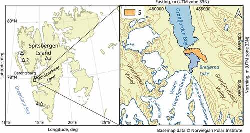
Meteorological data sets since 1933 are available from the weather station in Barentsburg (World Meteorological Organization station code 20,107, 75 m a.s.l.), approximately 15 km north-north-east of Vestre Grønfjordbreen. According to these data, the mean air temperatures for the four months from June through September were above zero from the beginning of the twenty-first century. Since 2000, the precipitation rate in Barentsburg has ranged between 495 and 795 mm per year, with a mean value of 580 mm, a maximum in December–January, and a minimum in June–July.

Some mass-balance data for Vestre Grønfjordbreen have been published before: the mass-balance years 2003/04–2005/06 (Solovyanova and Mavlyudov 2007) and 1965/66 and 1966/67 (WGMS 2019). These results could not be directly compared with the results of our study, as important metadata of the computations (ice density, exact survey dates, and the source of area–altitude distribution) were not reported, and no uncertainty limits were given.

Materials and methods

Glacier outlines

Glacier boundaries for two time points, corresponding to the start (2015) and end (2019) of the geodetic mass-balance calculations, were delineated. The boundary between Vestre Grønfjordbreen and Austre Dahlfonna is assumed to be constant and was taken from the Norwegian Polar Institute’s data set of glacier area outlines (König, Kohler, and Nuth 2013). The majority of the Vestre Grønfjordbreen margins (primarily the snout) were observed in August 2019 during a topographic survey, with cm-scale horizontal precision. However, steep slopes and crevasses made glacier margins in the upper part inaccessible to the ground-based survey; delineation here was therefore based on optical imagery with a best-available spatial resolution of 10 m from the Sentinel-2 satellite for 5 August 2019 (scene id L1C_T33XVG_A012605_20190805T124709). The computed area of the glacier at the end of the ablation period of 2019 equaled 16.42 ± 0.33 km².

To define the glacier area on 20 July 2015, we used an ArcticDEM data strip (Noh and Howat 2015; Porter et al. 2018). Despite the absence of the initial high-resolution imagery from which the digital elevation model (DEM) was derived, the significantly different terrain ruggedness of the glaciated and non-glaciated terrain made glacier delineation possible. The delineation process was aided by Landsat-8 pan-sharpened imagery taken on 9 July 2015, closest to the beginning of the geodetic differencing interval (scene id LC08_L1TP_215004_20150709_20170407_01_T1). The area for summer 2015 was estimated to be 16.76 ± 0.35 km².

GPR sounding

Fieldwork for GPR measurements was performed during April 2019, before the onset of surface melting. GPR profiles were obtained using the PulseEKKO PRO system with a 50 MHz dipole antenna. A Sokkia GRX2 GNSS system operating in real-time kinematic mode was used for horizontal and vertical positioning of each trace. The system was towed behind a snowmobile, driven at a speed of 5–8 km h⁻¹, the step between the traces was 0.5 m, and the coordinate frequency was 5 Hz. The total length of performed GPR profiles (Figure 3c) is 56 km, which is close to the total length of the previous soundings of 2010 (about 53 km). GPR data were processed using EKKO Project V5 (Sensors&Software) and visualized in OpendTect 6.4 (dGB Earth Sciences). Processing flow included sequentially: global navigation satellite system (GNSS)-receiver offset removal, correction of odometer-derived profile lengths based on GNSS measurements, normal move out correction, dewow and spatial background subtractions, F–K migration with a constant velocity of 170 m µs⁻¹, exponential signal gain to highlight target horizons, and time to depth conversion. At the last stage, the glacier bed and cold–temperate ice boundaries were picked manually.

Total glacier volume was computed after interpolation and extrapolation of ice-thickness profiles to the whole glacier surface. After testing several deterministic interpolation techniques implemented in open-source “SAGA GIS,” the “Thin Plate Spline” algorithm was chosen, since it resulted in a mean total volume from all the used methods. The thin plate spline, being the special case of a polyharmonic spline, is the two-dimensional analogue of the cubic spline in one dimension, which produces a smooth surface (a detailed description of the algorithm may be found in Bookstein (1989)). In our case, the regularization was applied to make the interpolant pass through the GPR data points exactly.

Glaciological mass balance

Annual mass balance

Annual mass balance (B_a) was determined from wooden stakes inserted up to 2.5 m deep in the ice. Stakes were installed along a single longitudinal profile on the primary snout (Figure 2a). Seven stakes were initially placed in the ice (drilled in September 2013), but the lowest stake (number 1) was lost in 2017 as a result of terminus retreat. Measurements were performed on a floating-date basis to keep mass changes within a single mass-balance year (Cogley et al. 2011). The precise dates of the start and end of observations depended on air temperature variability in each year and are shown in Table 1.

Table 1. Annual and seasonal glaciological mass balances of Vestre Grønfjordbreen in 2013/14–2019/2020.

Mass-balance year	Ba	Bw	Bs	Dates of Ba observations	Dates of Bw observations (snow survey)
	m w. e.
2013/14	–0.60 ± 0.18	0.67 ± 0.20	–1.27 ± 0.27	10 Sep 2013 – 26 Sep 2014	25 Apr 2014
2014/15	–0.88 ± 0.24	0.75 ± 0.23	–1.63 ± 0.33	26 Sep 2014 – 12 Sep 2015	05 May 2015
2015/16	–1.19 ± 0.21	0.36 ± 0.19	–1.56 ± 0.29	12 Sep 2015 – 12 Sep 2016	16 Apr 2016
2016/17	–1.92 ± 0.23	0.60 ± 0.19	–2.53 ± 0.30	12 Sep 2016 – 04 Sep 2017	09 Apr 2017
2017/18	–1.19 ± 0.22	0.44 ± 0.16	–1.63 ± 0.27	04 Sep 2017 – 18 Sep 2018	10 Apr 2018
2018/19	–0.78 ± 0.20	0.56 ± 0.31	–1.34 ± 0.36	18 Sep 2018 – 16 Sep 2019	02 May 2019
2019/20	–2.01 ± 0.26	0.48 ± 0.12	–2.46 ± 0.28	16 Sep 2019 – 23 Sep 2020	07 May 2020

Figure 2. (a) Observational network on Vestre Grønfjordbreen and (b) the profiles of the ground-based GNSS survey (2019): snow thickness sampling sites (1); snow pits (2); ablation stakes (3); GNSS survey profiles (4); and elevation contour lines for year 2015 (5).

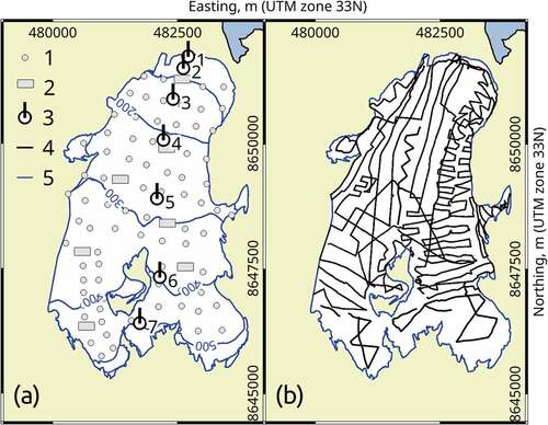
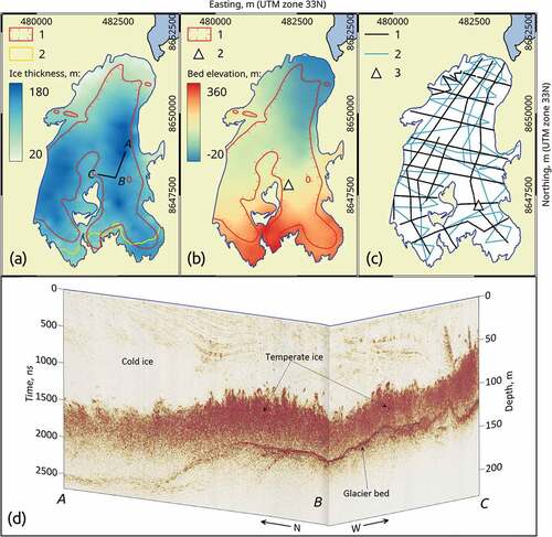
Figure 3. The results of the GPR study of Vestre Grønfjordbreen. (a) Ice thickness in April 2019: outlines of temperate ice (1); outlines of firn zone (2). (b) Bed elevations based on the GPR survey: outlines of temperate ice (1); minor ice fall (2). (c) Profiles of the GPR study: year 2019 (1); year 2010 (2); the deepest observed glacier ice (3). (d) The intersection of processed GPR lines (OpendTect 6.4 software was used for visualization).

A conventional profile method (Østrem and Brugman 1991; Kaser, Fountain, and Jansson 2003) was used to extrapolate point measurements and to obtain glacier-wide mass-balance values. The annual mass balance was computed for every 100 m altitudinal range using a linear fit, approximating the mass-balance profile from all the measured stakes. We modified the formula of glacier-wide balance computation by Tsutaki et al. (2017):

(1) $B=\sum \frac{S_z}{S}{b}_z=\sum W_z{b}_z,$(1)

where z represents the number of an elevation bin, S_Z/S is the ratio of the bin area to the total glacier area (dimensionless “weight” W_Z), and b_Z is the specific mass balance in the bin. Weights of elevation ranges in a total glacier-wide balance were based on area–altitude distribution. Ice density is assumed to be 850 ± 60 kg m^–3, as proposed by Huss (2013).

Annual mass balances for three years (2015/16–2017/18) have already been reported by Sidorova et al. (2019), but we have revised them and produced new homogenized values as newer, more accurate data sources appeared. First, the more relevant DEM, particularly ArcticDEM strips (Noh and Howat 2015; Porter et al. 2018) close to the beginning of the reported period (year 2015), was used. Second, we revised the coordinates of ablation stakes, which have been measured more precisely using DGPS methods. The altitudinal positions of the stakes differ by about 10–20 m from those defined previously in the study by Sidorova et al. (2019) with a hand-held Global Positioning System (GPS). We do not update stake coordinates from year to year, using the coordinates obtained in the end of melt season of 2018 for all the seven mass-balance years. We demonstrate further that stake displacements equal only several meters per year, and the uncertainty assessment indirectly takes into account this error source.

Seasonal mass balances

The winter balance (B_w) is computed from snow surveys, which are made at the end of every spring (precise dates are given in Table 1), as a product of mean snow thickness and depth-averaged density. The observational network, shown in Figure 2, is preserved from year to year and consists of seven snow pits (with two exceptions: six pits in the year 2019 and only three in 2020) distributed along the two supposed major flow lines. Snow density, measured layer by layer inside snow pits, is averaged by depth and is then averaged algebraically between pits and attributed to the whole glacier surface. Several dozen sampling points for snow thickness observations (80 points in 2014–2019 and 21 point in the year 2020) are located within a denser and quasi-regular network. Snow depth at these points is sampled with an avalanche probe, with an average of three measurements at each site. As most of the glacier becomes free of snow at the end of summer within the reported period, errors due to defining the last summer surface are considered to be negligible. Glacier-wide snow thickness is computed as a mean of all the depth measurements, which in the case of a regular network is the equivalent of linear interpolation.

While annual and winter mass balances are computed from in situ measurements, the summer balance B_s is defined as a residual by subtracting the winter balance from the annual balance.

Geodetic mass balance

The geodetic mass balance for Vestre Grønfjordbreen was calculated based on the difference between the results of a topographic survey made in August (the end of ablation season) 2019 and the ArcticDEM strip for year 2015. The first step for doing that is the calculation of the volume change, which, according to Zemp et al. (2013), is expressed as

(2) $\mathrm{\Delta }V=r^2{\sum }_{k=1}^k\mathrm{\Delta }{h}_k,$(2)

where r is the pixel size, k is the number of pixels involved in the volume change computation, and Δh_k is the elevation change in corresponding pixels of the differenced DEM. In order to convert glacier volume into mass change, a glacial ice density of 850 ± 60 kg m^–3 was used for both the geodetic and glaciological mass-balance computations. As an estimate of the vertical quality measure of the two DEMs used here, an normalized mean absolute difference (NMAD) statistical value introduced by Höhle and Höhle (2009) was used, which equals

$NMAD=b\cdot media{n}_j\left(\left|\mathrm{\Delta }{h}_j-m_{\mathrm{\Delta }h}\right|\right),$

where $\mathrm{\Delta }{h}_j$ denotes the individual errors j = 1, …, n and $m_{\mathrm{\Delta }h}$ is their median value. Scaling coefficient b = 1.4826 represents the 0.75 quantile of the normal distribution.

A ground-based survey was made on 12–19 August 2019 using the kinematic differential GNSS method using Sokkia GRX1 and GRX2 receivers. The survey covered the glacier surface itself and the area near the terminus, which became deglaciated since our monitoring started (Figure 2b). The uppermost and the steepest parts of the glacier were mostly inaccessible for detailed ground-based surveying because of multiple crevasses; however, several topographic profiles covering this area were done. The survey took a week, and to minimize the effects of melt during the work period and provide seamless linkages between each day’s results, the survey was performed from the top, where ablation had mostly ended, to the snout, contouring the edges on the last day. August 2019 was relatively cold: the first solid precipitation was observed on the glacier on 15 August. Melt rates close to zero were observed in late August and September at the ablation stakes, justifying the assumption that the topographic survey represents the end of the ablation season. All points with vertical precision coarser than 5 cm were excluded from further processing. To produce a DEM from the survey results spline interpolation was used. The 2 m pixel size was chosen to match the spatial resolution of the ArcticDEM, which was intended for geodetic differencing.

The only available strip of ArcticDEM that covered the area of interest without major gaps was derived from WorldView-2 satellite imagery obtained on 20 July 2015. This strip was pre-processed, which included interpolation of smaller gaps and vertical adjustment.

To perform the vertical adjustment of the ArcticDEM strip, three geodetic marks located around Grønfjorden and an elevation profile in the valley of Grønfjorddalen were used. Other techniques for DEMs coregistering are not suitable in the case, because the DEM created from the topographic survey results does not cover any stable terrain. To minimize spatial autocorrelation, 10 points at distances of more than 100 m from each other were randomly chosen from the profile, making the total number of used ground control points 13. After computing the median vertical difference between these ground control points and the ArcticDEM strip, the DEM was shifted by this value (−1.918 m).

Annual ice velocity

The annual surface ice flow velocity has been measured only once, by determining the displacement in horizontal plane of stakes number 2–6 (Figure 2a) between 1 August 2018 and 1 August 2019. DGPS equipment was used to perform fast static survey and obtain point coordinates at each stake. The observation time for each stake varied from 20 to 60 min depending on the number of satellites available and their configuration in the sky. Since the time span of the displacement is precisely one year, its value matches numerically the annual ice velocity.

Meteorological data

Meteorological data from the Barentsburg weather station, freely distributed by the Russian Institute of Hydrometeorological Information World Data Center (RIHMI–WDC), were obtained via the RIHMI–WDC website meteo.ru. Positive degree-day (PDD) amounts were computed from the data set of daily mean temperatures.

As an estimate of solid precipitation amounts, we used precipitation sums at the Barentsburg weather station from October to April; these are referred to below as “winter precipitation.” These months correspond to the period with negative mean monthly temperatures.

Uncertainty assessment

Glacier outlines

The uncertainties of the glacier area arising from the procedure of outline delineation were defined as the standard deviation of several manual digitizations from various analysts, as proposed by Paul et al. (2013). Despite the obvious retreat of the glacier terminus position since the beginning of monitoring (extending up to 200 m for the main trunk), confidence intervals of computed areas overlap considerably (16.76 ± 0.35 km² in 2015 and 16.42 ± 0.33 km² in 2019). Therefore, for all seven mass-balance years reported, we used a time-averaged value of 16.59 ± 0.24 km² in our computations of mass loss.

GPR sounding

Previous GPR studies of the glaciers around the bay of Grønfjorden (Martín-Español et al. 2013) show that during the early spring there is no significant spatial variability of the radio wave velocity (RWV) in different parts of a glacier. The RWV used for time-to-depth conversion was assumed constant, equaling 170 m μs⁻¹ ± 2 percent for the whole glacier surface, following Navarro and Eisen (2010). The errors of radar positioning performed by the GNSS kinematic method were assumed to be negligible since the typical errors of the horizontal and vertical positions are one or two orders of magnitude smaller than the depth measurement error. Other errors arising from GPR measurement are the uncertainty due to 3D-effects of so-called off-nadir or out-of-plane reflection, when the reflected wave is not received from the nadir but from a lateral glacier wall, and the uncertainty in picking the bedrock reflection in the GPR profiles. These two sources are hardly possible to quantify directly from the measurements themselves (Lapazaran et al. 2016). Hence, we estimated the error of a single measurement based solely on RWV uncertainty. However, the main contributors to the uncertainty of the total glacier volume (and therefore to the uncertainty of the mean ice thickness) are thought to be interpolation and extrapolation procedures. Performing these procedures using four different deterministic techniques (Natural Neighbor, Nearest Neighbor, Inverse Distance Weighting, Thin Plate Spline) led to different results of the total glacier volume. Propagating the standard deviation of these results and the assumed RWV error, we calculated the total uncertainty of the glacier volume. This value was estimated to be approximately 7%. For all the further computations the thickness grid obtained from Thin Plate Spline was chosen, since this algorithm resulted in a mean total volume from all the used methods.

Glaciological mass balance

Uncertainty assessment, not earlier reported in mass-balance studies of glaciers around Grønfjorden (e.g., Hagen and Liestøl 1990; Chernov et al. 2019; Sidorova et al. 2019; Elagina et al. 2021), is still a challenging task. Following Galos et al. (2017), we divided the errors in the glaciological budget by their sources in three main groups: (1) uncertainty related to the limited stake representativeness σ_point; (2) uncertainty of the model used for spatial averaging over the glacier σ_model; and (3) uncertainty of elevation bin areas σ_WZ. As these factors could not be quantified directly from measurements themselves, the uncertainty assessment involves some expert knowledge of the glacier (e.g., Andreassen et al. 2016; Klug et al. 2018).

Zemp et al. (2013) proposed accounting for one more factor influencing the total uncertainty of the direct mass balance: the uncertainty of the field measurements at point locations. It is caused by the stake sinking/floating or inclination, and not accounting for superimposed ice. However, recent studies regard this uncertainty as small compared to aforementioned uncertainties. Galos et al. (2017) suggested that random errors of ablation on the point scale equal 2–3 cm. Chernov et al. (2019) presents the similar value of 2 cm for the neighboring Austre Grønfjordbreen. Thus, we neglect this error source in our uncertainty assessment.

From Eqn. (1(1) $B=\sum \frac{S_z}{S}{b}_z=\sum W_z{b}_z,$(1) ), according to the rule of uncertainty propagation for a product of two independent variables (Fornasini 2008), the uncertainty of the mass-balance extrapolation over the whole glacier was

(3) ${\sigma }_{\mathrm{B}}^2=\sum W_z^2{\sigma }_{\mathrm{b}\mathrm{z}}^2+\sum b_z^2{\sigma }_{\mathrm{w}\mathrm{z}}^2,$(3)

where the uncertainty σ_bz of the mean specific mass balance in every elevation bin was computed by propagating the σ_point and σ_model values. To quantify the error of the mass-balance inhomogeneity after Galos et al. (2017) (σ_point), the results of our topographic survey were adopted. We took a value of 0.32 m as an estimate, as this value is the NMAD of the control point elevations measured in situ versus their elevations interpolated from the topographic survey. We assumed that this value represents the surface roughness of the studied glacier, characterizing the height of its surface features after the melt season. The error σ_model was estimated by taking the root mean square error of the real stake readings from the linear fit in a single year, as proposed by Fountain and Vecchia (1999). We suppose that the σ_model also indirectly assesses any imprecisions in ablation stake vertical coordinates. The uncertainty σ_WZ of the ratio of an elevation bin area to the whole glacier area was estimated on the basis of the accuracy of the glacier boundary delineation technique and was assumed not to exceed 0.02 (2 percent of the glacier surface) for each elevation interval.

The uncertainty of ice density is taken into account by a simple error propagation. If ρ is a conversion factor and B is the mass-balance result, then

(4) ${\sigma }_{\mathrm{B}\mathrm{w}\mathrm{e}}=B\sqrt{{\left(\frac{{\sigma }_{\rho }}{\rho }\right)}^2+{\left(\frac{{\sigma }_{\mathrm{B}}}{B}\right)}^2}\hspace{0.17em}.$(4)

The presence of systematic error in annual glaciological mass balances could only be identified retrospectively, based on intercomparison with geodetic mass balances.

Uncertainty assessment of the winter mass balance seems to be a more challenging task, since the observed spatial distributions of snow thickness or snow density do not show clear relationships with elevation above sea level or distance from center line. This implies that it is not possible to use any physical models for uncertainty assessment. We therefore estimate the error of the winter mass balance based on a simple approach, applied by Belart et al. (2017), among others, by propagating the standard deviations of area-averaged snow thickness and density. This technique yields uncertainty values similar to those of annual mass balances (around 0.20 m w.e.), but considering that the absolute B_w values are typically smaller than B_a values, the relative error of B_w is considerably higher and is up to 50 percent. Uncertainty of the summer balance is computed by propagating the uncertainties of annual and winter balances as the root of the sum of the squared annual and winter balances.

Geodetic mass balance

The variance of volume change, based on the rules of uncertainty propagation, is equal to

(5) $\begin{array}{c}{\sigma }_{\mathrm{\Delta }\mathrm{V}}^2=r^{4}k\left({\sigma }_{2015}^2+{\sigma }_{2019}^2\right),\end{array}$(5)

where σ₂₀₁₅ and σ₂₀₁₉ represent elevation uncertainties of the ArcticDEM strip and of the DEM derived from the topographic survey, respectively. We use the corresponding NMAD values, NMAD₂₀₁₅ and NMAD₂₀₁₉, instead of the variance as a more robust uncertainty measure (Höhle and Höhle 2009).

For computing NMAD₂₀₁₉, the vertical precision of a single GNSS measurement obtained from the post-processing procedure could not be directly used as a quality measure for the derived DEM, as a major part of the uncertainty typically comes from interpolation between points. Therefore, 40 control points on the glacier surface were measured after the topographic survey was completed. These points were located between collected topographic profiles and distributed on the glacier as evenly as possible. Based on these measurements, the NMAD₂₀₁₉ value for the interpolated DEM is 0.32 m.

To compute NMAD₂₀₁₅, the quality of the vertical reference of the 2015 ArcticDEM strip was estimated. This was done by computing the NMAD value between the ground control points vertical positions and the elevations of the corresponding pixels of the ArcticDEM fragment after vertical adjustment. This leads to an NMAD₂₀₁₅ value of 0.54 m.

Further, to translate the volume change into a conventional geodetic mass-balance value, the following equation was used:

(6) $\begin{array}{c}B=\frac{\mathrm{\Delta }V}{S}\rho ,\end{array}$(6)

where ΔV is the value found from Eqn. 2(2) $\mathrm{\Delta }V=r^2{\sum }_{k=1}^k\mathrm{\Delta }{h}_k,$(2) , S is the arithmetic average of the glacier area at the beginning and end of the differencing period, and ρ is the density conversion factor mentioned above. If we denote the ratio $\mathrm{\Delta }V/S$, which represents the spatially averaged elevation difference, as A, then its variance could be estimated in two ways, with and without accounting for the spatial autocorrelation of the DEM errors. The latter approach is simpler, being derived from the same error propagation rules, and may be expressed as follows:

(7) $\begin{array}{c}{\sigma }_{\mathrm{A}}^2=A^2\left({\left(\frac{{\sigma }_{\mathrm{\Delta }\mathrm{V}}}{\mathrm{\Delta }V}\right)}^2+{\left(\frac{{\sigma }_{\mathrm{S}}}{S}\right)}^2\right)\end{array}.$(7)

An alternative approach, which considers spatial autocorrelation, was proposed by Rolstad, Haug, and Denby (2009), and is represented by the following equation:

(8) ${\sigma }_{\mathrm{A}}^2=\frac{1}{5}{\sigma }_{\mathrm{\Delta }\mathrm{z}}^2\frac{S_{\mathrm{c}\mathrm{o}\mathrm{r}}}{S},$(8)

where σ²_ΔZ denotes the variance of the elevation difference, and S_cor is an effective correlated area, proportional to the correlation range. As it was defined from analysis of the semivariogram of the topographic profile on a stable terrain, the correlation range is approximately 350 m.

We tested both Eqns. (7)(7) $\begin{array}{c}{\sigma }_{\mathrm{A}}^2=A^2\left({\left(\frac{{\sigma }_{\mathrm{\Delta }\mathrm{V}}}{\mathrm{\Delta }V}\right)}^2+{\left(\frac{{\sigma }_{\mathrm{S}}}{S}\right)}^2\right)\end{array}.$(7) and (8(8) ${\sigma }_{\mathrm{A}}^2=\frac{1}{5}{\sigma }_{\mathrm{\Delta }\mathrm{z}}^2\frac{S_{\mathrm{c}\mathrm{o}\mathrm{r}}}{S},$(8) ) using their output to obtain the desired variance of the geodetic mass balance B, which is the same as

(9) ${\sigma }_{\mathrm{B}}^2=B^2\left({\left(\frac{{\sigma }_{\mathrm{A}}}{A}\right)}^2+{\left(\frac{{\sigma }_{\rho }}{\rho }\right)}^2\right).$(9)

Both approaches, with and without considering spatial autocorrelation, yielded almost equal uncertainty intervals for the geodetic mass balance: 0.39 m w.e. versus 0.40 m w.e. over the total geodetic differencing interval, or around 0.20 m w.e. per year.

Annual ice velocity

The instrumental accuracy of displacement uncertainty estimated during the GNSS post-processing procedure is better than ±0.05 m for the horizontal component. However, we double the uncertainty of each stake’s annual displacement and estimate the final accuracy to be ±0.10 m because of the difficulties of precise centering above the hole in which the stakes were set up. It is almost impossible to install the GNSS receiver straight above the center of the stake hole, especially in the case when the stake is high above the glacier surface and is well frozen. The imprecise centering adds several centimeters of error to the horizontal coordinates, extending the total uncertainty of the stake displacement computation beyond the instrumental error itself. This uncertainty value is still low relative to the measured annual displacements, as is discussed below.

Results and discussion

Thermal structure and ice thickness

Our GPR survey confirmed the polythermal structure of Vestre Grønfjordbreen, which was first discovered in 2010 (Martín-Español et al. 2013). This structure, with a basal layer of temperate ice, superimposed by cold ice, and a cold terminus, is common for Svalbard polythermal glaciers (Sevestre et al. 2015). The outlines of an underlying temperate ice layer are presented in Figure 3. Since this layer is being identified on GPR sections by numerous bright local hyperbolic reflections (Figure 3d), the cold–temperate transition surface (CTS) was contoured along the line that envelops the topmost points (vertices) of these reflections. Mean thickness of the temperate ice layer is 42 m, with a maximum of 152 m. The temperate ice is missing along the glacier edges, except its south-western part, where an ice divide with the neighboring Austre Dahlfonna glacier is located.

The spatial distribution of the ice depth, based on the results of the GPR survey of year 2019, is shown in Figure 3. Total ice volume is estimated to be 1.987 ± 0.139 km³, which corresponds to a mass of 1,709 ± 169 Mt. A comparison of the glacier volume and mean ice thickness with the previous GPR survey results of year 2010 (Martín-Español et al. 2013; Table 3) is largely uninformative with regard to volume changes. The uncertainty limits of the sounding appear to be too broad to reveal statistically significant changes within the nine-year period, which does not allow computation of the glacier mass balance for the reported time span. The ice volumes of 1.918 ± 0.146 km³ (2010) and 1.987 ± 0.139 km³ (2019) should therefore not be treated as the glacier growing.

Table 2. Cumulative mass losses of Vestre Grønfjordbreen computed by two methods.

Method	Period	Cumulative mass balance	Mass loss
		m w.e.	Mt
Direct	10 Sep 2013 – 23 Sep 2020	–7.67 ± 0.55	143.2 ± 9.8
Direct	25 July 2015 – 16 Sep 2019	–5.66 ± 0.48	94.6 ± 7.9
Geodetic	20 July 2015 – 26 Aug 2019	–5.52 ± 0.40	91.6 ± 13.1

Changes in the mean ice thickness could not be detected either. We found the uncertainty of ±1 m for the mean ice depth reported in Martín-Español et al. (2013) to be unreliably small and recomputed it according to the general error propagation rule based on the given uncertainties of the glacier volume and its area in 2010. The obtained value of 107 ± 12 m does not show a statistically significant difference from 119 ± 9 m (2019).

Lavrentiev et al. (2019) reprocessed the same GPR field data of the year 2010 and suggested an even smaller value of the glacier total volume: 1.617 ± 0.161 km³. This result would require the growth of the glacier between 2010 and 2019, which is not consistent with its constantly negative mass balance observed with a direct method. It should be noted that Lavrentiev et al. (2019) use another value of RWV velocity—168 m μs⁻¹—but this single factor could not explain such a large contradiction.

Several explanations of this mismatch could be proposed. The most trivial is that the two compared surveys had been carried out along different tracks (Figure 3c) and any of them might under-sample the glacier areas with the thinnest or the thickest ice. Another possible reason could be related to the uneven RWV within cold and temperate glacier layers. With the example of Bakaninbreen, Murray, Booth, and Rippin (2007) demonstrated that this difference could be significant for a Svalbard polythermal glacier. This implies that the reduction of the overlying cold-layer thickness due to constantly negative surface mass balance should cause a gradual decrease of the depth-averaged RWV from year to year. It is hard to account for this effect without organizing additional surveys, using, for example, the common-midpoint (CMP) method or borehole radar measurements.

We found it useful to compare maximum observed ice-thickness values because as single measurements they are not affected by interpolation errors, so their uncertainty limits are much narrower. The maximum ice thickness changed by 29 ± 6 m, from 215 ± 5 m (or 214 m according to Lavrentiev et al. (2019)) in 2010 to 186 ± 4 m in 2019. Though it is unlikely that these measurements were taken at the exact same location, the area of the maximum depths was still in the same part of the glacier (Figure 3c).

Basal topography and flow velocity

The bed elevation map is shown in Figure 3. The underlying topography consists of two main longitudinal troughs separated by a ridge, which is exposed as a nunatak in the upper part of the glacier. The largest ice thicknesses are a result of these troughs, and a maximal thickness of 186 ± 4 m was observed in the eastern one. In the lower part of the glacier (between stakes 4 and 5), the western trough flows into the eastern, making the ice flow turn. This is shown by the annual displacement of the lower stake (Figure 4), which differs markedly from those of the other stakes.

Figure 4. (a) Surface lowering in 2015–19: contour lines of surface lowering (1), 5 m interval; supposed main flow lines (2). (b) Annual flow velocities between 2018 and 2019: contour lines of bed inclination, 5° interval (1); stake velocities and directions (2).

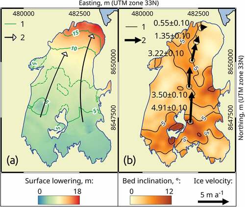
Annual stake displacements, observed between 2018 and 2019, become larger along the glacier flowline and vary from 0.50 ± 0.10 near the terminus to 4.50 ± 0.10 m near the nunatak. These low velocities are typical for terrestrial-terminating glaciers and are consistent with basal slopes; for example, beneath the fastest-moving stake (number 6), one of the steepest basal slopes occurs, and a minor ice fall is located on the glacier surface closer to the nunatak (Figure 3b).

We expect that the observed flow velocities are not truly representative of the whole glacier, as the existing stake profile is located between main flow lines, which we deduce from topography (Figure 4). Therefore, the observed stake displacement may underestimate the overall ice flow velocity.

Since we have only one annual interval of stake displacement observations, it is still unknown if the ice flow velocities of Vestre Grønfjordbreen vary from year to year and to which extent. Many of Svalbard’s glaciers are of the surge type (the estimated percentage varies between 15 and 90 percent, see Wangensteen, Weydahl, and Hagen 2005), which makes regular glacier velocity monitoring even more important. Kokin and Kirillova (2017) proposed that a rapid movement of Vestre Grønfjordbreen glacier could have occurred during the LIA, creating a push moraine consisting of marine sediments. However, no surges of the glacier have been documented since observations started at the beginning of the twentieth century.

Glaciological and geodetic mass balances

The annual (Ba), winter (Bw), and summer (Bs) balances for Vestre Grønfjordbreen and the exact survey dates, quantifying the duration of the ablation period, are reported in Table 1. All the annual balances for the reported period of seven years are negative, with the least negative budget in 2013/14 and most negative in 2019/20. Mass-balance profiles are shown in Figure 6.

Figure 5. Pit-averaged snow density values for Vestre Grønfjordbreen in 2014–2020.

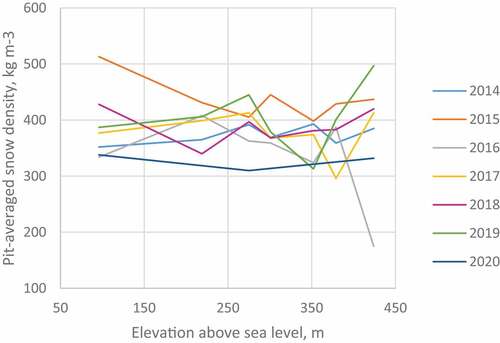
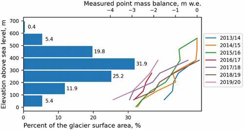
Figure 6. Area-altitude distribution for Vestre Grønfjordbreen (averaged between 2015 and 2019) and mass-balance profiles measured by glaciological method.

Point annual mass balances measured at the ablation stakes and their coordinates are shown in the Supplementary Tables S1 and S2. One or two upper ablation stakes, located in the eastern cirque, became inaccessible at the end of almost every ablation season because of exposed crevasses and moulins, making measurements from those stakes unavailable for most mass-balance years, which weakens the stake layout. As the linear approximation of the vertical mass-balance profile is used to extrapolate the measured values in the upper ranges of the glacier, while the real profile may be curved, this may become a source of the systematic bias in the record. Further the absence of the bias is demonstrated by a comparison with the results of the geodetic method.

While point annual mass-balance values depend on altitude, the same is not true for the winter balances. Since there is no altitudinal dependence for the pit-averaged snow densities (Figure 5), the mean of all snow pit bulk densities was used to compute glacier-wide B_w values.

According to our visual observations, for the last two decades, almost the whole surface of Vestre Grønfjordbreen has been free from snow cover at the end of the ablation season. A ratio of the snow remnant to the total glacier area varied from zero (2019/20) to ca. 27 percent (2018/19). Some areas with firn are still present above 540–550 m a.s.l., but their extent is limited to about 3–4 percent of the glacier surface, as it was delineated from the results of our GPR study (Figure 3).

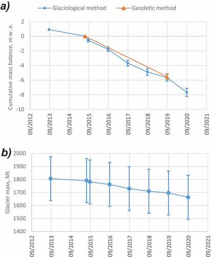
The cumulative mass balance for seven years is estimated to be -7.67 ± 0.55 m w.e., which corresponds to an overall mass loss of 143.2 ± 9.8 Mt (Table 2). This value equals roughly 8 ± 1 percent of the total glacier mass computed from our GPR survey. Comparing two values of Vestre Grønfjordbreen cumulative mass losses during the period of 2014/15–2018/19, obtained by two different methods (Table 2), allows for a cross-check for a systematic bias in a mass-balance series. Assuming that basal and internal accumulation and ablation are negligible and the same are the density changes of the surface layer, glacier-wide values of geodetic and glaciological mass balance should coincide (Fischer 2011; Galos et al. 2017). In our study, these two values are equal at a significance level of 95 percent and, consequently, there is no significant systematic bias between them (Figure 7). The uncertainty related to the shift of five days between the start dates of the direct observations and geodetic differencing is also assumed to be negligible. We therefore conclude that a calibration of the glaciological record is not needed.

Table 3. Comparison between GPR results for the years 2010 and 2019.

		Ice volume	Mean (area-averaged) ice thickness	Maximum observed ice thickness
Year	Source	km^3	m	m
2010	Martín-Español et al. (2013)	1.918 ± 0.146	107 ± 12	215 ± 5
2010, reprocessed	Lavrentiev et al. (2019)	1.617 ± 0.161	94	214
2019	This study	1.987 ± 0.139	119 ± 9	186 ± 4
Change		n/a^a	n/a^a	–29 ± 6

^aChange is statistically insignificant (α = 0.05).

Figure 7. (a) Cumulative mass loss of Vestre Grønfjordbreen and (b) total glacier mass (b) for the period 2013/14–2019/20.

Relationship between mass balance and meteorological conditions

Numerous studies show (e.g., Gardner et al. 2011; Van Pelt et al. 2021) that Arctic glaciers are sensitive to summer temperatures, which could be quantified by mean summer temperature or positive degree-day sums. Lefauconnier and Hagen (1990), based on a 22-year record of direct observations from Austre Brøggerbreen, in north-western Spitsbergen, showed that the net balance is also closely correlated with winter precipitation. We therefore computed correlations with annual PDD and with winter precipitation. We found PDD more informative than mean monthly/seasonal temperatures, as it has a larger interannual variance at the study site.

The correlation between annual mass balance (B_a) and PDD is negative but weak, equaling only –0.44 (Figure 8a). The correlation between summer mass balance (B_s) and PDD is also negative but with an even lower correlation factor equaling –0.33 (Figure 8b). Being squared, these numbers provide coefficients of determination (R²), which show the proportion of the variation in the dependent variable that is predictable from the independent variable. Given these numbers, one could conclude that only 19 percent of the interannual variability of B_a and only 11 percent of B_s are explained by PDD year-to-year differences. This might be true, since regional climate is not the only driver of interannual variability of the annual mass balance. Other factors such as microclimate, albedo, debris cover, ice thickness, and geometry of a glacier (Florentine et al. 2018; Moore, Nelson, and Groth 2019) affect both melt and accumulation processes.

Figure 8. Scatterplots between mass-balance values of Vestre Grønfjordbreen and meteorological parameters at the Barentsburg weather station: (a) annual mass balances and positive degree-day sums; (b) summer mass balances and positive degree-day sums; (c) winter mass balance and precipitation amounts during October–April; (d) annual mass balances and winter mass balances.

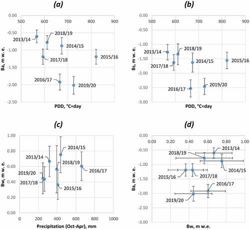
The correlation between winter balance (B_w) and precipitation in October–April is positive but weak: 0.36 (Figure 8c). In comparison, Hagen and Liestøl (1990) reported a correlation for Austre Brøggerbreen of 0.63 and treated this value as low. Considering the fact that the Ny-Ålesund weather station is located in the immediate vicinity of Austre Brøggerbreen, while the distance between the Vestre Grønfjordbreen terminus and the Barentsburg weather station is about 15 km, the lower correlation coefficient for the latter case is reasonable. However, Grabiec (2005), extending the ideas of Førland and Hanssen-Bauer (2000), proposed another possible explanation of a weak correlation for B_w, which relates to the errors in recorded winter precipitation amounts due to the technical difficulties of measuring solid precipitation on station gauges. This instrument-related error behaves non-linearly, becoming larger with increasing wind speed and with decreasing temperature (Grabiec 2005). On the other hand, accumulation processes on a glacier are controlled by local factors, such as glacier topography, orography of the surrounding ridges, snowdrift, and precipitation inversions.

One more correlation test between B_a and B_w was performed, related to the possible influence of snow accumulation on the summer melt: the thicker the snow cover is, the longer it maintains the high albedo of the glacier surface during summer, preserving underlying material from ablation (Van Pelt, Pohjola, and Reijmer 2016). The correlation coefficient value is positive, as expected, but small: 0.40 (Figure 8d).

Demonstrated relationships between seasonal and annual mass balances and the meteorological records from the Barentsburg weather station are straightforward and expected, but correlation values are not very high. Annual mass-balance value for 2015/16 seems to be a serious outlier (Figure 8). This mass-balance year was extreme in terms of both temperature and solid precipitation: PDD value was the highest during the monitoring period, while the preceding winter had resulted in the least snow accumulation. However, annual mass balance is not the most negative in the series and not even comparable with the most negative observed ones (2016/17 and 2019/20). We treat the error in the computations of a glacier-wide value for 2015/16 unlikely. On the one hand, all the stakes were measured (none of them was unreachable), which excludes a serious bias from extrapolation using a linear fit. On the other hand, the difference of about 0.7–0.8 m w.e. relative to the most negative years is too large to arise from a single erroneous field note. If we omit the annual mass-balance value for 2015/16 from the analysis, all the correlation coefficients are improved drastically: from −0.44 to −0.75 for B_a–PDD, from −0.33 to −0.80 for B_s–PDD, and from 0.40 to 0.51 for B_w–B_a. The hypothesis for explaining the apparently outlying balance year is that the Barentsburg meteorological station may experience different local weather conditions than the areas to the south and south-west of Grønfjorden bay, missing some wind patterns and temperature fluctuations that affect Vestre Grønfjordbreen (Florentine et al. 2018; Mott, Stiperski, and Nicholson 2020).

Comparison with the other Svalbard glaciers

Based on the available data on annual glaciological mass balances (WGMS 2019; Elagina et al. 2021), a simple correlation test could be done to compare the B_a interannual variability of Vestre Grønfjordbreen and seven other land-terminating Svalbard glaciers with at least five mass-balance years of observations: Austre Brøggerbreen, Midtre Lovénbreen, Irenebreen and Waldemarbreen located in Oscar II Land (Spitsbergen), Svenbreen to the north of the settlement of Pyramiden, and Werenskioldbreen in the southern part of Spitsbergen Island (Figure 1). The choice of glaciers to compare with Vestre Grønfjordbreen is constrained by the presence of ongoing studies and on data availability and does not account for possible similarities or discrepancies in local factors, such as surface topography, aspect of snout exposition, ice thickness, and debris coverage.

Correlation coefficients for B_a since the start of our monitoring program in the mass-balance year 2013/14 are shown in Table 4. Considering the brevity of the record from Vestre Grønfjordbreen, it could be useful to illustrate the extent to which the coefficient is affected by shortening the sample. Therefore, we also computed correlation coefficients for the other glaciers, using all the overlapping observational periods for each pair (sample size is limited to the minimum observational series length in each pair). These results are presented in Table 4.

Table 4. Matrix of pair correlation coefficients for annual mass balances of land-terminating Svalbard glaciers: a) for the period of 2013/14–2018/19, b) for the maximum available overlapping monitoring period; total length of observational series (in mass-balance years) is indicated for each glacier in parentheses.

a)	Vestre Grønfjordbreen	Austre Grønfjordbreen	Austre Brøggerbreen	Midtre Lovénbreen	Irenebreen	Waldemarbreen	Svenbreen	Werenskioldbreen
Vestre Grønfjordbreen	-	0.08	0.52	0.52	0.65	0.51	0.29	0.51
Austre Grønfjordbreen	0.08	-	0.76	0.73	0.39	0.50	0.71	0.80
Austre Brøggerbreen	0.52	0.76	-	1.00	0.86	0.91	0.96	0.99
Midtre Lovénbreen	0.52	0.73	1.00	-	0.85	0.91	0.96	0.97
Irenebreen	0.65	0.39	0.86	0.85	-	0.98	0.81	0.84
Waldemarbreen	0.51	0.50	0.91	0.91	0.98	-	0.91	0.88
Svenbreen	0.29	0.71	0.96	0.96	0.81	0.91	-	0.91
Werenskioldbreen	0.51	0.80	0.99	0.97	0.84	0.88	0.91	-
b)	Vestre Grønfjordbreen	Austre Grønfjordbreen	Austre Brøggerbreen	Midtre Lovénbreen	Irenebreen	Waldemarbreen	Svenbreen	Werenskioldbreen
Vestre Grønfjordbreen (6)	-	0.08	0.52	0.52	0.65	0.51	0.29	0.51
Austre Grønfjordbreen (16)	0.08	-	0.63	0.65	0.63	0.71	0.50	0.60
Austre Brøggerbreen (53)	0.52	0.63	-	0.98	0.58	0.61	0.75	0.93
Midtre Lovénbreen (52)	0.52	0.65	0.98	-	0.62	0.63	0.69	0.95
Irenebreen (17)	0.65	0.63	0.58	0.62	-	0.96	0.79	0.87
Waldemarbreen (24)	0.51	0.71	0.61	0.63	0.96	-	0.73	0.85
Svenbreen (8)	0.29	0.50	0.75	0.69	0.79	0.73	-	0.65
Werenskioldbreen (7)	0.51	0.60	0.93	0.95	0.87	0.85	0.65	-

Several results are notable: a very tight correlation exists between the B_a of glaciers situated in neighboring valleys—Austre Brøggerbreen and Midtre Lovénbreen, Irenebreen and Waldemarbreen—and this is true for both the last seven mass-balance years and for the whole overlapping periods. The same correlation of B_a did not occur between neighboring Vestre Grønfjordbreen and Austre Grønfjordbreen.

Analysis of the time series of mass-balance measurements (Figure 9) shows that Vestre Grønfjordbreen did not experience the negative mass-balance peak observed for most of the other glaciers in the sample in 2015/16. As discussed above, the annual mass-balance value of Vestre Grønfjordbreen for that year seems to be an anomalous value, and Figure 9 clearly shows that such behavior also differs markedly from the other glaciers. On the other hand, Vestre Grønfjordbreen is not entirely unique in the sample: the mass balance of the glacier Irenebreen does not seem to vary significantly within the years 2014/15–2017/18, making this the row that correlates best with Vestre Grønfjordbreen. These two glaciers have little in common in terms of their morphometry; Vestre Grønfjordbreen is about four times larger and faces north-east instead of north-west, so we are not able to propose any common local factor explaining the absence of the negative peak of 2015/16. On a sub-regional scale, any features of the atmospheric or maritime circulation should obviously affect Austre Grønfjordbreen and Vestre Grønfjordbreen in a similar manner.

Figure 9. Interannual variability of land-terminating Svalbard glaciers: (a) poorly correlated with Vestre Grønfjordbreen; (b) better correlated with Vestre Grønfjordbreen.

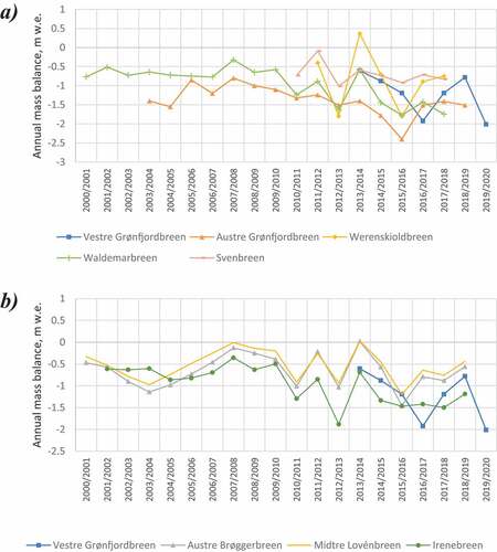
A closer look to the beginning and end dates of the annual mass-balance measurements on Austre Grønfjordbreen may explain the poor correlation with the neighboring Vestre Grønfjordbreen. Glaciological mass-balance values presented in the study by Elagina et al. (2021)—the same data reported to the World Glacier Monitoring Service (WGMS)—do not follow the conventional mass-balance year system and could cover the time spans for example from August to August. While the start and end dates of the mass-balance year 2016/17 are more or less consistent with ours, the year 2015/16—with an apparent peak of the negative mass balance—includes the whole August and September of the previous year. This attributes the mass loss of Austre Grønfjordbreen, including approximately one and a half melting seasons, to a single balance year. Other mass-balance years are also shifted relative to those we are using in this study, complicating a meaningful comparison. One thing that can be concluded, though, is that the mass-balance series of both Austre Grønfjordbreen and Vestre Grønfjordbreen show poor correlation with other Svalbard glaciers. As a possible explanation of the different glacier interannual variability in this area, we can only suggest the stronger influence of warm Atlantic Water inflow, as described, for example, for the Hornsund fjord (Arntsen et al. 2019), but the lack of relevant measurements renders this hypothesis very speculative.

Conclusion

We report the homogenized seven-year record of direct annual and seasonal mass-balance measurements on Vestre Grønfjordbreen from 2013/14 to 2019/20. All seven reported values of the annual balance were negative and vary from –0.60 ± 0.18 to –1.92 ± 0.23 m w.e. Correlation tests between mass-balance values and meteorological parameters yielded expected results, but the coefficients were not very high, possibly because of local on-glacier weather conditions not captured by the Barentsburg weather station. Comparing five of the reported mass-balance years with the results of geodetic differencing, we conclude that there is no significant systematic bias in direct observations. To date, this is the second series of ongoing direct mass-balance observations in the Barentsburg area (after the Austre Grønfjordbreen) coupled with geodetic validation. In contrast to the earlier study, our results include an uncertainty assessment.

Acknowledgments

The authors are grateful to the Russian Arctic Expedition on Svalbard (Arctic and Antarctic Research Institute, Saint Petersburg, Russia) for providing logistics and GNSS equipment and for helping to carry out the field studies. The ArcticDEM strip used in this study was created from DigitalGlobe, Inc. imagery. We thank the European Space Agency for making the Sentinel-2 imagery used in the study to delineate glacier outlines freely available. ‬‬‬‬‬‬‬‬‬

Supplemental data

Supplemental data for this article can be accessed online at https://doi.org/10.1080/15230430.2022.2150122.

Disclosure statement

No potential conflict of interest was reported by the author(s).

Additional information

Funding

This study was funded under Project 5.1.4, Monitoring of State and Pollution of the Environment, Including the Cryosphere, in the Arctic Basin and in the Area of Scientific Station Ice Base Cape Baranov, Hydrometeorological Observatory of Tiksi and Russian Scientific Centre on Spitsbergen, within the Plan NITR of Roshydromet Project 5.1.4 within the Plan NITR of Roshydromet 2020–24 2020–24. ArcticDEM strip used in this study was created from DigitalGlobe, Inc., imagery and provided by the Polar Geospatial Center under NSF-OPP awards [1043681, 1559691, and 1542736].

References

- Andreassen, L. M., H. Elvehøy, B. Kjøllmoen, and R. V. Engeset. 2016. Reanalysis of long–term series of glaciological and geodetic mass balance for 10 Norwegian glaciers. The Cryosphere 10:535–602. doi:10.5194/tc-10-535-2016.
- Arntsen, M., A. Sundfjord, R. Skogseth, M. Błaszczyk, and A. Promińska. 2019. Inflow of warm water to the inner Hornsund fjord, Svalbard: Exchange mechanisms and influence on local sea ice cover and glacier front melting. Journal of Geophysical Research—Oceans 124:1915–31. doi:10.1029/2018JC014315.
- Belart, J. M. C., E. Berthier, E. Magnússon, L. S. Anderson, F. Pálsson, T. Thorsteinsson, I. M. Howat, G. Aðalgeirsdóttir, T. Jóhannesson, and A. H. Jarosch. 2017. Winter mass balance of Drangajökull ice cap (NW Iceland) derived from satellite sub-meter stereo images. The Cryosphere 11:1501–17. doi:10.5194/tc-11-1501-2017.
- Bloshkina, E. V., A. K. Pavlov, and K. Filchuk. 2021. Warming of Atlantic Water in three west Spitsbergen fjords: Recent patterns and century-long trends. Polar Research 40:5392. article no. doi:10.33265/polar.v40.5392.
- Bookstein, F. L. 1989. Principal warps: Thin plate splines and the decomposition of deformations. IEEE Transactions on Pattern Analysis and Machine Intelligence 11:567–85. doi:10.1109/34.24792.
- Chernov, R. A., A. V. Kudikov, T. V. Vshivtseva, and N. I. Osokin. 2019. Estimation of the surface ablation and mass balance of Eustre Grønfjordbreen (Spitsbergen). Led i Sneg 59 (1):59–66. (In Russian with English title and abstract.). doi:10.15356/2076-6734-2019-1-59-66.
- Cogley, J. G., R. Hock, L. A. Rasmussen, A. A. Arendt, A. Bauder, R. J. Braithwaite, P. Jansson, G. Kaser, M. Möller, L. Nicholson, et al. 2011. Glossary of glacier mass balance and related terms. IHP-VII. Technical Documents in Hydrology 86. IACS Contribution 2. Paris: United Nations Educational, Scientific and Cultural Organization.
- Elagina, N., S. Kutuzov, E. Rets, A. Smirnov, R. Chernov, I. Lavrentiev, and B. Mavlyudov. 2021. Mass balance of Austre Grønfjordbreen, Svalbard, 2006–2020, estimated by glaciological, geodetic and modeling aproaches [sic]. Geosciences 11:78. article no. doi:10.3390/geosciences11020078.
- Fischer, A. 2011. Comparison of direct and geodetic mass balances on a multi-annual time scale. The Cryosphere 5:107–24. doi:10.5194/tc-5-107-2011.
- Florentine, C., J. Harper, D. Fagre, J. Moore, and E. Peitzsch. 2018. Local topography increasingly influences the mass balance of a retreating cirque glacier. The Cryosphere 12:2109–22. doi:10.5194/tc-12-2109-2018.
- Førland, E. J., and I. Hanssen–Bauer. 2000. Increased precipitation in the Norwegian Arctic: True or false? Climatic Change 46:485–509. doi:10.1023/A:1005613304674.
- Fornasini, P. 2008. The uncertainty in physical measurements: An introduction to data analysis in the physics laboratory. Berlin: Springer.
- Fountain, A. G., and A. Vecchia. 1999. How many stakes are required to measure the mass balance of a glacier? Geografiska Annaler, Series A: Physical Geography 81:563–73. doi:10.1111/1468-0459.00084.
- Galos, S. P., C. Klug, F. Maussion, F. Covi, L. Nicholson, L. Rieg, W. Gurgiser, T. Mölg, and G. Kaser. 2017. Reanalysis of a 10-year record (2004–2013) of seasonal mass balances at Langenferner/Vedretta Lunga, Ortler Alps, Italy. The Cryosphere 11:1417–39. doi:10.5194/tc-11-1417-2017.
- Gardner, A., G. Moholdt, B. Wouters, G. J. Wolken, D. O. Burgess, M. J. Sharp, J. G. Cogley, C. Braun, and C. Labine. 2011. Sharply increased mass loss from glaciers and ice caps in the Canadian Arctic Archipelago. Nature 473:357–60. doi:10.1038/nature10089.
- Grabiec, M. 2005. An estimation of snow accumulation on Svalbard glaciers on the basis of standard weather-station observations. Annals of Glaciology 42:269–76. doi:10.3189/172756405781812808.
- Hagen, J. O., and O. Liestøl. 1990. Long-term glacier mass-balance investigations in Svalbard, 1950–1988. Annals of Glaciology 14:102–06. doi:10.3189/S0260305500008351.
- Höhle, J., and M. Höhle. 2009. Accuracy assessment of digital elevation models by means of robust statistical methods. ISPRS Journal of Photogrammetry and Remote Sensing 64:398–406. doi:10.1016/j.isprsjprs.2009.02.003.
- Huss, M. 2013. Density assumptions for converting geodetic glacier volume change to mass change. The Cryosphere 7:877–87. doi:10.5194/tc-7-877-2013.
- Isaksen, K., Ø. Nordli, E. J. Førland, E. Łupikasza, S. Eastwood, and T. Niedźwiedź. 2016. Recent warming on Spitsbergen—influence of atmospheric circulation and sea ice cover. Journal of Geophysical Research—Atmospheres 121:11913–31. doi:10.1002/2016JD025606.
- Kaser, G., A. G. Fountain, and P. Jansson. 2003. A manual for monitoring the mass balance of mountain glaciers with particular attention to low latitude characteristics. Paris: United Nations Educational, Scientific and Cultural Organization.
- Klug, C., E. Bollmann, S. P. Galos, L. Nicholson, R. Prinz, L. Rieg, R. Sailer, J. Stötter, and G. Kaser. 2018. Geodetic reanalysis of annual glaciological mass balances (2001–2011) of Hintereisferner, Austria. The Cryosphere 12:833–49. doi:10.5194/tc-12-833-2018.
- Kokin, O. V., and A. V. Kirillova. 2017. Reconstruction of Grønfjordbreen dynamics (west Spitsbergen) in the Holocene. Led i Sneg 57 (2):241–52. (In Russian, with English title and summary.). doi:10.15356/2076-6734-2017-2-241-252.
- König, M., J. Kohler, and C. Nuth. 2013. Glacier area outlines—Svalbard. Tromsø: Norwegian Polar Institute.
- Kotljakov, V. M., ed. 1985. Glaciology of Spitsbergen. Moscow: Nauka.
- Lapazaran, J., J. Otero, A. Martín-Español, and F. Navarro. 2016. On the errors involved in ice-thickness estimates I: Ground-penetrating radar measurement errors. Journal of Glaciology 62 (236):1008–20. doi:10.1017/jog.2016.93.
- Lavrentiev, I. I., A. F. Glazovsky, Y. Y. Macheret, V. V. Matskovsky, and A. Y. Muravyev. 2019. Reserves of ice in glaciers on the Nordenskiöld Land, Spitsbergen, and their changes over the last decades. Led i Sneg 59 (1):23–38. (In Russian, with English title and summary.). doi:10.15356/2076-6734-2019-1-23-38.
- Lefauconnier, B., and J. Hagen. 1990. Glaciers and climate in Svalbard: Statistical analysis and reconstruction of the Brøggerbreen mass balance for the last 77 years. Annals of Glaciology 14:148–52. doi:10.3189/S0260305500008466.
- Macheret, Y. Y., A. F. Glazovsky, I. I. Lavrentiev, and I. O. Marchuk. 2019. Distribution of cold and temperate ice in glaciers on the Nordenskiold Land, Spitsbergen, from ground-based radio-echo sounding. Ice and Snow 59 (2):149–66. (In Russian, with English title and summary.). doi:10.15356/20766734-2019-2-430.
- Martín-Español, A., E. Vasilenko, F. Navarro, J. Otero, J. Lapazaran, I. Lavrentiev, Y. Y. Macheret, and F. Machío. 2013. Radio-echo sounding and ice volume estimates of western Nordenskiöld Land glaciers, Svalbard. Annals of Glaciology 54:211–17. doi:10.3189/2013AoG64A109.
- Mavljudov, B. R., and I. J. Solov’janova. 2007. Vodno–ledovyj balans lednika Al’degonda v 2003/03 balansovom godu.(Water–ice balance of Aldegondabreen glacier during the 2002/03 balance year). Materialy Glatsiologicheskikh Issledovaniy 102:206–08.
- Möller, M., and J. Kohler. 2018. Differing climatic mass balance evolution across Svalbard glacier regions over 1900–2010. Frontiers in Earth Science 6:128. article no. doi:10.3389/feart.2018.00128.
- Moore, P. L., L. I. Nelson, and T. M. D. Groth. 2019. Debris properties and mass-balance impacts on adjacent debris-covered glaciers, Mount Rainier, USA. Arctic, Antarctic, and Alpine Research 51:70–83. doi:10.1080/15230430.2019.1582269.
- Mott, R., I. Stiperski, and L. Nicholson. 2020. Spatio-temporal flow variations driving heat exchange processes at a mountain glacier. The Cryosphere 14:4699–718. doi:10.5194/tc-14-4699-2020.
- Murray, T., A. Booth, and D. M. Rippin. 2007. Water-content of glacier-ice: Limitations on estimates from velocity analysis of surface ground-penetrating radar surveys. Journal of Environmental and Engineering Geophysics 12:87–99. doi:10.2113/JEEG12.1.87.
- Navarro, F., and O. Eisen. 2010. Ground-penetrating radar in glaciological applications. In Remote sensing of glaciers: Techniques for topographic, spatial and thematic mapping of glaciers, ed. P. Pellikka and W. G. Reese, 195–229. London: Taylor & Francis.
- Nilsen, F., R. Skogseth, J. Vaardal-Lunde, and M. Inall. 2016. A simple shelf circulation model: Intrusion of Atlantic Water on the West Spitsbergen Shelf. Journal of Physical Oceanography 46:1209–30. doi:10.1175/JPO-D-15-0058.1.
- Noël, B., C. L. Jakobs, W. J. J. van Pelt, S. Lhermitte, B. Wouters, J. Kohler, J. O. Hagen, B. Luks, C. H. Reijmer, W. J. van de Berg, et al. 2020. Low elevation of Svalbard glaciers drives high mass loss variability. Nature Communications 11:4597. article no. doi:10.1038/s41467-020-18356-1.
- Noh, M., and I. M. Howat. 2015. Automated stereo-photogrammetric DEM generation at high latitudes: Surface extraction with TIN-based search-space minimization (SETSM) validation and demonstration over glaciated regions. GIScience and Remote Sensing 52:198–217. doi:10.1080/15481603.2015.1008621.
- Nordli, Ø., R. Przybylak, A. Ogilvie, and K. Isaksen. 2014. Long-term temperature trends and variability on Spitsbergen: The extended Svalbard Airport temperature series, 1898–2012. Polar Research 33:21349. article no. doi:10.3402/polar.v33.21349.
- Nuth, C., J. Kohler, M. König, A. von Deschwanden, J. O. Hagen, A. Kääb, G. Moholdt, and R. Pettersson. 2013. Decadal changes from a multi-temporal glacier inventory of Svalbard. The Cryosphere 7:1603–21. doi:10.5194/tc-7-1603-2013.
- Østrem, G., and M. Brugman. 1991. Glacier mass-balance measurements: A manual for field and office work. NHRI Science Report 4, Saskatoon: National Hydrology Research Institute, Environment Canada.
- Paul, F., N. Barrand, S. Baumann, E. Berthier, T. Bolch, K. Casey, H. Frey, S. P. Joshi, V. Konovalov, R. Le Bris, et al. 2013. On the accuracy of glacier outlines derived from remote-sensing data. Annals of Glaciology 54:171–82. doi:10.3189/2013AoG63A296.
- Porter, C., P. Morin, I. Howat, M. J. Noh, B. Bates, K. Peterman, S. Keesey, M. Schlenk, J. Gardiner, K. Tomko, et al. 2018. ArcticDEM., Version 1. Harvard Dataverse, Polar Geospatial Center, University of Minnesota. Accessed May 20, 2020. https://dataverse.harvard.edu/dataset.xhtml?persistentId=doi:10.7910/DVN/OHHUKH
- Rolstad, C., T. Haug, and B. Denby. 2009. Spatially integrated geodetic glacier mass balance and its uncertainty based on geostatistical analysis: Application to the western Svartisen ice cap, Norway. Journal of Glaciology 55:666–80. doi:10.3189/002214309789470950.
- Schuler, T., J. Kohler, N. Elagina, J. O. Hagen, A. Hodson, J. Jana, A. Kääb, B. Luks, J. Małecki, G. Moholdt, et al. 2020. Reconciling Svalbard glacier mass balance. Frontiers in Earth Science 8:156. article no. doi:10.3389/feart.2020.00156.
- Sevestre, H., D. I. Benn, N. R. J. Hulton, and K. Bælum. 2015. Thermal structure of Svalbard glaciers and implications for thermal switch models of glacier surging. Journal of Geophysical Research: Earth Surface 120:2220–36. doi:10.1002/2015JF003517.
- Sidorova, O. R., G. V. Tarasov, S. R. Verkulich, and R. A. Chernov. 2019. Surface ablation variability of mountain glaciers of west Spitsbergen. Arctic and Antarctic Research 65: (In Russian with English title and summary): 438–48. doi:10.30758/0555-2648-2019-65-4-438-448.
- Skogseth, R., L. L. A. Olivier, F. Nilsen, E. Falck, N. Fraser, V. Tverberg, A. B. Ledang, A. Vader, M. O. Jonassen, J. Søreide, et al. 2020. Variability and decadal trends in the Isfjorden (Svalbard) ocean climate and circulation—an indicator for climate change in the European Arctic. Progress in Oceanography 187:102394. article no. doi:10.1016/J.POCEAN.2020.102394.
- Solovyanova, I. Y., and B. R. Mavlyudov. 2007. Mass balance observations on some glaciers in 2004/2005 and 2005/2006 balance years, Nordenskiöld Land, Spitsbergen. In The dynamics and mass budget of Arctic glaciers. Extended abstracts. Workshop and GLACIODYN (IPY) Meeting 15-18 January 2007, Pentresina (Switzerland). IASC Working Group on Arctic Glaciology, 115–20. Utrecht: Institute for Marine and Atmospheric Research Utrecht. https://nag.iasc.info/images/publications/abstracts/Book_IASC-NAG2017.pdf
- Troitsky, L. S., E. M. Singer, V. S. Koryakin, V. A. Markin, and V. I. Mikhailov. 1975. Glaciation of the Spitsbergen (Svalbard): Results of researches of international geophysical projects. Moscow: Nauka.
- Tsutaki, S., S. Sugiyama, D. Sakakibara, T. Aoki, and M. Niwano. 2017. Surface mass balance, ice velocity and near-surface ice temperature on Qaanaaq Ice Cap, northwestern Greenland, from 2012 to 2016. Annals of Glaciology 58:181–92. doi:10.1017/aog.2017.7.
- Van Pelt, W. J. J., J. Oerlemans, C. H. Reijmer, V. A. Pohjola, R. Pettersson, and J. H. van Angelen. 2021. Simulating melt, runoff and refreezing on Nordenskiöldbreen, Svalbard, using a coupled snow and energy balance model. The Cryosphere 6:641–59. doi:10.5194/tc-6-641-2012.
- Van Pelt, W., V. Pohjola, R. Pettersson, S. Marchenko, J. Kohler, B. Luks, J. O. Hagen, T. V. Schuler, T. Dunse, B. Noël, et al. 2019. A long-term dataset of climatic mass balance, snow conditions, and runoff in Svalbard (1957–2018). The Cryosphere 13:2259–80. doi:10.5194/tc-13-2259-2019.
- Van Pelt, W., V. Pohjola, and C. Reijmer. 2016. The changing impact of snow conditions and refreezing on the mass balance of an idealized Svalbard glacier. Frontiers in Earth Science 4:2296–6463. doi:10.3389/feart.2016.00102.
- Wangensteen, B., D. J. Weydahl, and J. O. Hagen. 2005. Mapping glacier velocities on Svalbard using ERS tandem DInSAR data. Norwegian Journal of Geography 59:276–85. doi:10.1080/00291950500375500.
- WGMS. 2019. Fluctuations of glaciers database. Zurich: World Glacier Monitoring Service.
- Zemp, M., E. Thibert, M. Huss, D. Stumm, C. Rolstad Denby, C. Nuth, S. U. Nussbaumer, G. Moholdt, A. Mercer, C. Mayer, et al. 2013. Reanalysing glacier mass balance measurement series. The Cryosphere 7:1227–45. doi:10.5194/tc-7-1227-2013.