Three-dimensional subsurface architecture and its influence on the spatiotemporal development of a retrogressive thaw slump in the Richardson Mountains, Northwest Territories, Canada

ABSTRACT

The development of retrogressive thaw slumps (RTS) is known to be strongly influenced by relief-related parameters, permafrost characteristics, and climatic triggers. To deepen the understanding of RTS, this study examines the subsurface characteristics in the vicinity of an active thaw slump, located in the Richardson Mountains (Western Canadian Arctic). The investigations aim to identify relationships between the spatiotemporal slump development and the influence of subsurface structures. Information on these were gained by means of electrical resistivity tomography (ERT) and ground-penetrating radar (GPR). The spatiotemporal development of the slump was revealed by high-resolution satellite imagery and unmanned aerial vehicle–based digital elevation models (DEMs). The analysis indicated an acceleration of slump expansion, especially since 2018. The comparison of the DEMs enabled the detailed balancing of erosion and accumulation within the slump area between August 2018 and August 2019. In addition, manual frost probing and GPR revealed a strong relationship between the active layer thickness, surface morphology, and hydrology. Detected furrows in permafrost table topography seem to affect the active layer hydrology and cause a canalization of runoff toward the slump. The three-dimensional ERT data revealed a partly unfrozen layer underlying a heterogeneous permafrost body. This may influence the local hydrology and affect the development of the RTS. The results highlight the complex relationships between slump development, subsurface structure, and hydrology and indicate a distinct research need for other RTSs.

KEYWORDS:

• Retrogressive thaw slump
• permafrost
• spatiotemporal slump development
• near-surface geophysics
• remote sensing

Introduction

Ongoing global warming and the associated changes in regional climatic patterns have strong impacts on arctic regions, leading to significantly faster warming compared to the global average and changing precipitation patterns (Intergovernmental Panel on Climate Change 2021). Especially in areas characterized by the presence of permafrost, these changes lead to hydrological and thermal feedbacks in the subsurface, accompanied by an increasing active layer thickness (ALT) and changing water pathways. Along with this, an increasing number and activity of retrogressive thaw slumps (RTS) has been detected in many parts of the Arctic and especially in northwestern Canada (Lantuit and Pollard 2008; S. V. Kokelj et al. 2015; Segal, Lantz, and Kokelj 2016; Lewkowicz and Way 2019) and Alaska (Balser, Jones, and Gens 2014; Balser 2015; Swanson and Nolan 2018). RTSs are backwasting thermokarst features and represent one of the most rapid erosion processes in the present periglacial environments on earth (French 2017). In comparison to other periglacial landforms, they are rather short-lived, with an average activity period of thirty to fifty years (French and Egginton 1973), but in this time, they lead to sometimes enormous mass redistributions. Extreme rainfall events have major impacts on RTS initialization and their growth rates. Accordingly, in wet summers with more heavy rainfall events, the formation of new RTSs is more frequent and the growth rates of existing slumps are significantly higher (S. V. Kokelj et al. 2015; Lewkowicz and Way 2019).

Recent studies on RTSs focused on the impact of slumps on river systems regarding material transport (S. V. Kokelj et al. 2013, 2021) and geo- and biochemistry (Littlefair, Tank, and Kokelj 2017; Shakil et al. 2020; Zolkos et al. 2020; Bröder et al. 2021) but also on the spatiotemporal slump development using Earth observation data (Brooker et al. 2014; Segal, Lantz, and Kokelj 2016; Lewkowicz and Way 2019; Nitze et al. 2021). Further studies highlighted the influence of various terrain parameters, deduced from digital elevation models (DEMs), on the slump development (Lacelle et al. 2015; Ramage et al. 2017; Ward Jones, Pollard, and Jones 2019). Studies of RTSs employing geophysical surveying are rare so far but the methods are able to provide key information on the subsurface properties; for example, in regions adjacent to retreating headwalls. This subsurface information increases the knowledge about local permafrost properties and (permafrost) hydrology. Both factors have been inadequately studied in RTS environments, although they have major influences on spatiotemporal slump development. Local hydrology is of particular interest because it links both catchment areas of slump sites and downstream water bodies and can increase the spatial influence of local slump sites to larger scales due to sediment cascades and geo- and biochemical impacts (S. V. Kokelj et al. 2021).

The current study uses a combined approach of remote sensing and geophysical methods to investigate the spatiotemporal development and local subsurface structures adjacent to the retreating headwall of a RTS at the edge of the Richardson Mountains (Canada). The spatiotemporal development is investigated using satellite images as well as high-resolution unmanned aerial vehicle (UAV)-based orthoimages and digital DEMs. Manual frost probing, electrical resistivity tomography (ERT), and ground-penetrating radar (GPR) are used to reveal subsurface structures and to gather information on the ALT and ice contents of the permafrost in the surrounding of the slump. The investigations focus on the relationships between local hydrology, subsurface structure, and the spatiotemporal slump behavior, thus providing a holistic view on the different environmental conditions and processes.

Study site

The Peel Plateau, located in the southwest of the Mackenzie Delta (Northwest Territories, Canada), is well known for widespread and ice-rich permafrost often containing ground ice of glacial origin. This is due to its former position at the marginal zone of the Laurentide Ice Sheet (LIS), which reached its maximum limit at the edge of the Richardson Mountains at approximately 18 ka cal yr BP (Lacelle et al. 2013, 2015). Consequently, glaciofluvial, glaciolacustrine, and glacial sediments of a hummocky moraine terrain dominate the surficial geology of the Peel Plateau up to an elevation of approximately 750 m.a.s.l. (Duk-Rodkin 1992; S. V. Kokelj et al. 2015). The adjacent Richardson Mountains, reaching an altitude of up to 1,575 m.a.s.l., were ice-free and belonged to the ice-free sector of Beringia (Lacelle et al. 2013). The geology of the mountain range is characterized by Cretaceous (Jurassic) and Devonian shales and siltstones (Wheeler et al. 1996; Yukon Geological Survey 2020) and the slopes and valleys are mostly covered by colluvial material. The current climate at the climate station Fort McPherson (approximately 50 km northeast of the study site, 35 m.a.s.l.) is characterized by a mean annual air temperature of −7.3°C and a mean annual precipitation of 298 mm (rainfall: 145.9 mm; snowfall: 152.5 cm, 1981–2010; Government of Canada 2020). Within the Richardson Mountains there are no long-term climatic measurements, but the data of a climate station installed 14 km to southwest of the study site suggests a slightly warmer mean annual air temperature of −5.4°C ± 0.9°C at an altidue of 660 m.a.s.l. between 2014 and 2021 (S. A. Kokelj et al. 2022). Recent studies indicated that atmospheric inversion settings during winter months caused average temperatures in the Peel Plateau and adjacent Richardson Mountains to be warmer than in Fort McPherson, which is located on the Peel Plain (O’Neill et al. 2015). In the last three decades, the total amount of summer precipitation and also the number of extreme precipitation events increased significantly in this region (S. V. Kokelj et al. 2015). Permafrost is continuous in this region and permafrost temperatures derived from large-scale data sets are between −2°C and −5°C (Brown, Sidlauskas, and Delinski 1997; Henry and Smith 2001). Recent studies recorded warmer permafrost temperatures (−1°C to −3°C) than expected by the aforementioned large-scale models due to the inversion-related warmer winter temperatures and a rather fast snow accumulation on tundra vegetation (shrubs; O’Neill et al. 2015). The thickness of permafrost ranges between 120 m close to Fort McPherson (Mackay 1967) and up to 625 m in higher elevations in the Richardson Mountains close to the Yukon–Northwest Territories border. Therefore, permafrost thicknesses of about 300 m are suspected for the higher elevated parts of the Peel Plateau region (Smith, Meikle, and Roots 2004). The region is known for the widespread occurrence of RTSs due to the degradation of ice-rich permafrost. At least ten of them are classified as megaslumps due to their size of more than 20 ha (Lacelle et al. 2015).

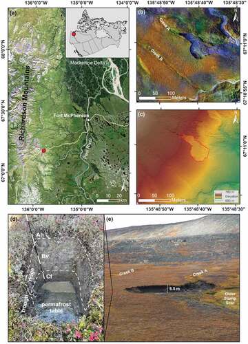
The investigated RTS (67°10′59″, −135°48′41″; Figure 1) is located at the eastern flank of the Richardson Mountains in the transition zone toward the Peel Plateau and close to the Dempster Highway (km 25 from NWT border). It is situated on a southeast-exposed slope at an altitude of about 730 m.a.s.l. and is separated by a small creek (Creek A; cf. Figure 1) from an older slump scar. The old scar is already covered with vegetation and seems to be stable (see Figure 1e). The creek is part of the Vitrekwa Creek catchment, is deeply incised in some areas, and currently runs right through the slump floor. The area of the slump is just under 6,000 m² (September 2021) and the retreating headwall is up to 6.5 m in height. Therefore, the investigated slump is rather small compared to other slumps in the region, which are characterized by an average size of 5.4 ha (Lacelle et al. 2015). However, because the slump is comparatively young and the slump type and initiation seem to be similar to others in the region, the slump appears to be quite representative. After Duk-Rodkin (1992), the location of the slump is exactly at the edge of the LIS and, therefore, the slump developed in glaciogenic materials containing ice-rich permafrost. According to the ground ice map of O’Neill, Wolfe, and Duchesne (2022), the study site is underlain by ice-rich permafrost with an ice content between 20 and 30 percent. The exposed permafrost at the headwall shows strongly varying ice contents on a small scale, which, however, are higher than the abovementioned 20 to 30 percent in some areas. Due to slope-parallel stone stripes, the near-surface subsurface is characterized by alternating substrates. Whereas the dominating part is characterized by clay and silt dominated fine-grained material, the other part mainly consists of loamy sediments containing also pebbles. Whereas the fine-grained material forms hummock-like ridges, the coarser material is situated in troughs inbetween. After the World Reference Base classification, the soil type has to be classified as Cambic Turbic Cryosol. The frost sorting-related substrate differences also affect the vegetation coverage. The fine-grained ridges are covered by a mixture of dwarf shrubs (willows and birches), grass, herbs, and lichens, whereas the troughs underlain by loamy sediments are covered by moss almost exclusively. Recent remote sensing–based studies indicated a greening trend within the region caused by shrub expansion (Fraser et al. 2014; Nill et al. 2019, 2022), which can also affect the thermal regime in the subsurface on a long-term scale.

Figure 1. (a) Location of the study site in the transition zone between the Richardson Mountains and the Peel Plateau indicated by the red dot. The cloud-free Landsat-8 RGB true-color image composite was provided by Nill et al. (2019). (b), (c) High-resolution unmanned aerial vehicle (UAV)-based orthoimage and digital elevation model. The area of erosion by the slump is surrounded by the red line. The white dots in (c) mark the electrode positions of the electrical resistivity tomography (ERT) measurements. (d) A soil profile (image curtesy: L. Nill) and (e) a ground-based photo of the retrogressive thaw slumps (RTS) and its surrounding taken on 4 September 2019. Both the active slump in the central part of the image and the stabilized and already vegetation-covered slump in the right part of the image are visible. The position of (d) is marked in (e).

Materials and methods

A combined approach of geophysical and remote sensing methods was applied to investigate the development of the RTS and its relationship to the prevailing subsurface properties such as active layer thickness, substrate properties, and ice content.

Remote sensing methods

The remote sensing methods include a UAV-based structure from motion approach performed two times (2018 and 2019) in the area of the slump as well as a manual mapping of the slump area based on optical satellite images (2014–2021).

UAV-based structure from motion

During two field campaigns in August 2018 and August 2019, two UAV surveys were conducted to generate aerial images of the slump area. The UAV used was a DJI Phantom 3 Pro equipped with a standard camera (12.4 MP, 1/2.3-in. complementary metal oxide semiconductor sensor). The flights were each piloted manually so that an overlap of 80 percent in flight direction with a sidelap of approximately 60 percent was reached. Three different flight heights above ground (approximately 30, 60, and 90 m) were accomplished during both surveys to reach an acceptable spatial resolution and coverage. After sorting out blurred or distorted images, a total number of 180 (25 August 2018) and 937 (23 August 2019) images were used for further processing, taking into account that the surveyed area was much larger in 2019. The aerial images were used in a structure from motion approach using the software Agisoft PhotoScan Professional (Agisoft 2016). Six well-visible and unchanged positions in the study area were used as reference points for the calibration and coregistration of the two models. For this purpose, features like striking boulders or distinct features in microrelief were used, which seem to be stable throughout the period of investigation. Nevertheless, a detailed survey of these points using real-time kinematic positioning was not possible. Therefore, there is a certain uncertainty in this regard that should be discussed later on. The subsequent processing contained the image alignment, the identification of ground control points (GCPs), and the camera optimization. Afterward a dense point cloud was created, out of which a mesh, a DEM, and an orthoimage were computed. The derived models were characterized by spatial resolutions between 3 and 4 cm and were resampled to an resolution of 5 cm to enable a comparison of the data sets.

To investigate the changes between the two timesteps, morphometric analysis was performed in ArcMap (ESRI Inc. 2018) as well as in the software Geomorphic Change Detection 7 (GCD 7; Bailey et al. 2020), v7.5.0.0. The detailed methodological approach of the GCD 7 software is described in Wheaton (2008), Wheaton, Brasington, Darby, and Sear (2010), and Wheaton, Brasington, Darby, Merz et al. (2010).

Slump development monitoring

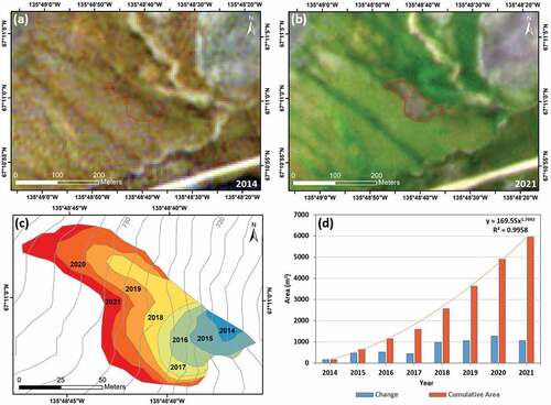
The development of the slump was investigated using high-resolution optical satellite images from RapidEye and PlanetScope (Planet Labs PBC). Based on eight scenes acquired between 2014 and 2021, the yearly development of the slump was mapped manually using true-color RGB (red–green–blue) composites. The scenes (Table 1) provided a spatial resolution of 3 × 3 m or 5 × 5 m per pixel, were cloud-free, and were acquired in late August or early September. No data at appropriate resolution were available before 2014. Because the erosion processes are of particular interest in this study, the cumulative area and the annual change were restricted to the scar zone of the slump. Changes in the accumulation zone further downslope were not taken into account when looking at spatial changes.

Table 1. List of used remote sensing scenes for long-term slump development analysis.

Date	Satellite	Scene ID	Resolution
9 September 2014	RapidEye-5	20140909_214033_870113_RapidEye-5	5 × 5 m
6 July 2015	RapidEye-5	20150706_213703_870113_RapidEye-5	5 × 5 m
24 August 2016	Planet Scope	20160824_194908_0e20	3 × 3 m
16 August 2017	Planet Scope	20170816_200004_0e0f	3 × 3 m
29 August 2018	Planet Scope	20180829_200733_1012	3 × 3 m
9 September 2019	Planet Scope	20190909_173053_1054	3 × 3 m
29 August 2020	Planet Scope	20200829_184412_62_106a	3 × 3 m
5 August 2021	Planet Scope	20210805_194447_14_245d	3 × 3 m

Hydrological modeling

Based on the TanDEM-X DEM (10-m resolution; created in 2011/2012) and on the UAV-derived DEM, a modeling of the surface hydrology was conducted using the System for Automated Geoscientific Analyses (SAGA) software v7.2.0 (Conrad et al. 2015). The processing included fill sinks after L. Wang and Liu (2006), flow accumulation (flow tracing; Gruber and Peckham 2009), and SAGA wetness index calculation after Böhner et al. (2002). The same processing was applied to two elevation models of the permafrost table topography derived from (1) the frost probing and (2) GPR measurements to investigate the influence of the local hydrology. Therefore, permafrost table was picked manually in the GPR data and its depth values were exported every 0.5 m along the profiles. The generated point cloud and the data points derived from frost probing were used to build two separate raster data sets containing the ALT. In a first step, the ALT was subtracted from the real elevation derived from the UAV-based DEM. The interpolation method used for subsequent generation of the raster data was spline interpolation conducted in ArcMap (ESRI Inc. 2018). The resolution of both data sets was set to 0.2 m taking into account that the original point density of the two data sets was quite different.

In situ and geophysical methods

In addition to the remote sensing analysis and the hydrological modeling, in situ measurements were conducted to investigate the subsurface structure adjacent to the retreating headwall of the RTS.

Frost probing

Manual frost probing was performed using a 120-cm-long steel rod to measure the ALT in the surrounding of the RTS and to calibrate the geophysical models. The steel rod was pushed into the soil until the frost table was reached. Because the measurements were carried out at the end of thaw season in late August and early September, it was assumed that the active layer had reached its seasonal maximum. As such, the measured depth was interpreted to represent the depth of the permafrost table. The measurements were rounded to an accuracy of 5 cm.

Ground-penetrating radar

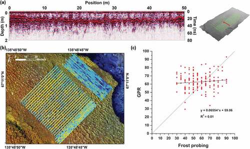
The use of GPR is widespread in the field of permafrost research and the method has often been used for ALT mapping (Hinkel et al. 2001; Moorman, Robinson, and Burgess 2003; Chen et al. 2016; Campbell et al. 2021) but also for the investigation of subsurface structures such as ice wedges within ice-rich permafrost (Munroe et al. 2007). The method is well suited for the detection of ALT because it is sensitive to dielectric differences between unfrozen and frozen state. A bistatic setup with a pair of antennas (i.e., transmitter and receiver) was employed using a PulsEKKO Pro System with unshielded 100-MHz antennas and a NOGGIN System with shielded 250-MHz antennas, both from Sensors and Software Inc. The three-dimensional (3D) grid consists of twenty-six parallel common-offset profiles performed with 250-MHz antennas and twenty-four common-offset profiles performed using 100-MHz antennas. For the best adjustment of signal propagation velocities during processing, they were first calculated by alignment with colocated frost probing results using the known two-way travel time of the signal and ALT. The subsequent GPR data processing included a time zero correction, background removal, dewow filtering, migration, SEG2 gaining, and a topographic correction of the data.

Electrical resistivity tomography

The ERT method is common in the field of permafrost research and is based on the different electrical resistivities of different materials. It enables the delineation of frozen and unfrozen materials as well as the detection of relative changes in water content or ice saturation (Kneisel et al. 2008; Reynolds 2011). Recently, the use of quasi-three-dimensional (q3D) approaches has enabled large-scale 3D surveying of subsurface heterogeneities within periglacial landforms (Emmert and Kneisel 2021; Kunz and Kneisel 2021). As such, the approach allows the investigation of the internal structure of geomorphological features and landforms. The q3D approach describes the measurement of several parallel or orthogonal profiles that are merged and inverted together afterward. This approach enables a detailed 3D investigation of larger areas in comparison to real 3D approaches (Rödder and Kneisel 2012; Hauck 2013).

To investigate the area surrounding the RTS, a grid of twenty-three profiles was surveyed using a Syscal Pro Switch 72 device from IRIS Instruments Inc. The measurement setup consists of ten longitudinal profiles measured with seventy-two electrodes and two additional longitudinal profiles as well as eleven cross-profiles measured with thirty-six electrodes. The electrode spacing used was 3 m and a dipole–dipole array was applied. The chosen interline spacing was 6 m between longitudinal profiles and 12 m between cross-profiles. The location of the individual profile lines is visible in Figure 1c. The data processing was conducted using the software packages RES2DINVx64 v4.05.41 (Geotomo Software SDN BHD 2015) and RES3DINVx64 v3.11.73 (Geotomo Software SDN BHD 2016). It included the removal of poor datum points based on a 5 percent threshold of the stack deviation and a two-dimensional (2D) trial inversion with subsequent bad datum point filtering based on a 100 percent root mean square error threshold as promoted by Loke (2019). Afterward, all 2D data were collated into a 3D data set and topography derived from UAV surveys was added. For the inversion, the L1-norm (robust inversion) with an initial damping factor of 0.1 and a vertical to horizontal flatness filter ratio of 1 was applied to the data.

Results

Spatiotemporal slump development

Long-term development

Based on the remote sensing data sets, the spatial development of the slump could be delineated for the period from August 2014 to July 2021 (Figure 2). The cumulative area in Figure 2 refers exclusively to the scar zone, the area in which erosion has taken place due to slump processes. The change describes the annual change in this area. At the beginning of the time series, the extent of the slump was around 160 m². That represents an initial state of the RTS and is close to the lowermost limit that could be detected visually using optical satellite data with the available resolutions. In the following years, the slump extended in a western and southwestern direction, but since 2018, the expansion has taken place along a small creek (Creek A) in a northwestern and northern direction. In contrast, the southward growth decreased significantly since 2018 and south of the initial slump scar. Since 2018, the annual spatial growth of the slump has increased significantly. This is likely due to the increasing area of the retreating headwall especially along Creek A. Along the incised creek, headwall retreat has taken place on both sites of the creek since 2018, which is why the headwall length was much higher and annual change has increased significantly since then. The cumulative area of the slump shows an exponential growth that can be seen in Figure 2d by the dotted line and the corresponding growth function, due to the increasing annual change. In the case of the growth shown for 2021, it should be noted that the extent was already measured in July and thus in the middle and not toward the end of the thaw season.

Figure 2. Spatial development of the retrogressive thaw slumps (RTS) between August 2014 and July 2021 derived from optical satellite data. At the top are two optical satellite images from (a) September 2014 (Image © 2014 Planet Labs PBC) and (b) August 2021 (Image © 2021 Planet Labs PBC). A red line in both images marks the 2021 extent of the area where erosion has taken place. (c) The temporal development of the slump and statistics on the annual change and (d) the cumulative spatial change.

High-resolution change detection

The two UAV surveys from August 2018 and August 2019 allowed the detection of small-scale variabilities of slump development and indicated the differences regarding erosion and accumulation. Differences between the two high-resolution DEMs of the entire slump area as well as the changes along two profiles are shown in Figure 3. The backward erosion of the headwall between the two surveys is colored in dark red and clearly visible. In this area, a negative vertical change of the surface of up to 6.5 m is observed. This also corresponds to the height of the headwall in August 2019. In contrast, in parts of the 2018 slump floor as well as along the course of the creek, an accumulation of material mainly took place, raising the slump floor by 1.0 to 1.4 m. This change also matches the change in headwall height, which was up to 7.5 m in August 2018 and thus 1 m higher than in 2019. Other portions of the slump floor, as well as much of the downslope areas outside the current stream channel, were balanced/stable during the observation period. However, individual features in the slump floor, representing larger root balls of former vegetation that have broken off the headwall, were slightly displaced toward the east. This is visible due to an increase in elevation of the eastern side and a decrease in elevation of the western side. This is also visible in profile A–A′ in Figure 3b. In addition, the two profiles in Figures 3b and 3c indicate the displacement of the headwall. The horizontal displacement was in a range between 4 and 7 m along the entire headwall length. At the spur protruding from the slump, the horizontal retreat was up to 11 m, because erosion in this area occurred from two sides. Profile B–B′ additionally shows the distinct widening of the erosion channel along both sides of the creek.

Figure 3. (a) Surface elevation changes within the affected area between 25 August 2018 and 23 August 2019 derived from two unmanned aerial vehicle (UAV)-based surveys. (b), (c) The surface elevation through the most active parts of the retrogressive thaw slumps (RTS) along the profile lines indicated in (a).

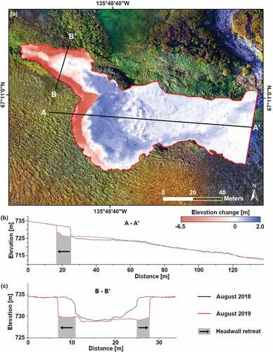
A numerical analysis of the two terrain models using GCD 7 software showed that the described changes correspond to an erosion of about 6,170 m³ and a redeposition of 4,970 m³ of material. Accordingly, about 1,200 m³ of material has been eroded and deposited outside the investigated area (approximately 20 percent). This volume includes the meltwater of the former ground ice draining into the channel and eroded sediment.

Subsurface architecture

Active layer characteristics and hydrology

The spatial distribution of the ALT in the area southwest of the slump adjacent to its retreating headwall was investigated using manual frost probing and GPR measurements. In Figure 4, the results of frost probing are shown as point data on the left and as interpolated spatial data on the right. The main result of these measurements is a clear zonation of the ALT depending on the relief position. The higher elevated positions on the slope between the two incised creeks are characterized by low ALTs between 15 and 60 cm, whereas the creeks in the southwestern part (Creek B) and also at the northern most edge of the grid (Creek A) are characterized by higher ALTs of up to 120 cm and more. The ALTs at the slope dipping toward Creek B are in a medium range between 60 and 85 cm but are separated from the creek by a small band of lower ALTs between 20 and 60 cm (cf. P1 in Figure 4b). This band runs parallel to the creek, approximately 10 m away from its center and is just a few meters wide. In the area of the slope ridge, which is predominantly characterized by low ALTs, a smaller cluster of somewhat higher ALTs is noticeable in the direction of the slump. This apparent gully-like structure in the permafrost table is also evident in the interpolated data, where it stands out as a brighter greenish to yellowish path running in the direction of the slump (P2 in Figure 4b). Similar structures are visible further downslope, one of which also drains toward the slump (P3 in Figure 4b).

Figure 4. Manual frost probing results of the area adjacent to the retreating headwall in early September 2019 shown (a) as point data and (b) spatially interpolated data. Positions referred to in the text are marked by dashed lines and labeled (P1–P3).

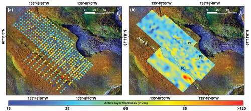
Comparing the frost probing data with GPR results (Figure 5), it is noticeable that the GPR data appear much more heterogeneous. At this point, it should be noted that the two data sets do not show a significant correlation (cf. Figure 5c), which will be discussed further. Especially in the 2D GPR profiles, a strongly undulating structure of the permafrost table is visible, which can be recognized in the data as an intense continuous reflector. This undulating structure coincides with the impressions from the field, where strong small-scale differences could also be detected during frost probing and within the soil pit shown in Figure 1d. However, these are not visible in the comparatively coarse-scaled grid in Figure 3. GPR data measured perpendicular to the slope direction indicate that the permafrost table has a system of furrows and ridges orientated in the direction of the slope. In addition to the topography of the permafrost table, the reflection characteristics within the active layer are striking. On top of the ridges, the reflections are much more intense than over the depressions in the permafrost table. These differences are indicative of substrate variations within the active layer occurring in a more or less regular pattern, which is the result of frost sorting processes and represents the already mentioned stone stripes. In particular, this changing pattern and the ridge and depression structures occur in the central part of the slope but not in the area immediately to the retreating headwall. In this area (approximately 5 m from the headwall), the permafrost table is more regular and the ALT is much lower (approximately 30–60 cm).

Figure 5. Results of ground-penetrating radar (GPR)-based active layer measurements. (a) A GPR profile of the 250 MHz antennas is shown for example. A red line highlights the continuous reflector of the frost table. The location of the profile in comparison to the electrical resistivity tomography (ERT) grid is shown on the right. (b) A map of derived active layer depth data (scale as in Figure 4). (c) A comparison between the frost probing results and the closest GPR-derived data points is visible as a scatterplot.

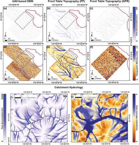
Figure 6 shows the results of hydrological modeling based on the UAV-derived DEM as well as on the permafrost table topography derived from frost probing and GPR. In Figures 6g and 6h, a large-scale analysis for the entire catchment area is shown to demonstrate the overall hydrological situation (from TanDEM-X DEM). The modeling based on the permafrost table topography derived from both methods (frost probing and GPR) shows a strong runoff canalization toward the RTS. In the permafrost table–based models, more runoff flows into the slump than in the models derived from the UAV surface models. The GPR-derived model presents a much more heterogeneous structure and seems more similar to the UAV-derived surface model due to the high resolution. Nevertheless, the flow directions are closer to those in the coarser permafrost table model derived from frost probing, so the GPR results demonstrate the altered hydrology due to the permafrost table topography.

Figure 6. (a)–(c) Calculated flow accumulation and (d)–(f) topographic wetness index based on the (a), (d) unmanned aerial vehicle (UAV)-derived digital elevation models (DEM), (b), (e) frost probing–derived frost table topography, and (c), (f) ground-penetrating radar (GPR)-derived frost table topography. The extent of the GPR data is marked in (a)–(f) by the dashed line. (g), (h) The hydrology of the larger catchment area based on the TanDEM-X DEM.

Permafrost characteristics

The underlying permafrost, investigated by ERT, shows a heterogeneous structure similar to the ALTs. Figure 7 presents selected depth slices of the q3D ERT model as a stacked layer graphic. Based on the frost probing results, the threshold value for the delineation between frozen and unfrozen ground seems to be around 600 Ωm. The first depth slice covers the uppermost 1.05 m of the model and seems to be affected by the varying active layer characteristics. Hence, this layer shows spatial variable patterns comparable to those revealed by frost probing. The small, incised channel (Creek B) is characterized by very low resistivity values (<100 Ωm), and the adjacent hillslope (P1 in Figure 7) also shows comparably low resistivity values (100–250 Ωm). In contrast, most parts of the slope (especially, the uppermost part; P2 in Figure 7) are characterized by resistivities between 600 and 1,800 Ωm. These differences might be due to different soil moistures within the active layer and also due to ALT variations. The uppermost model layer of the ERT integrates over the uppermost 1.05 m of the subsurface. In areas with ALTs higher than this, the model layer is unfrozen, whereas some parts of the model layer are frozen in areas with ALTs lower than the model layer thickness. In the upper hillslope area (P2), the higher resistivity values therefore might be affected by the lower ALTs in this area. Close to Creek B, where the uppermost model layer represents only unfrozen and saturated material, the resistivity values are distinctly lower.

Figure 7. Selected depth slices of the 3D electrical resistivity tomography (ERT) model. The threshold for delineation of frozen and unfrozen areas is around 600 Ωm. Positions referred to in the text are labeled (P1–P4).

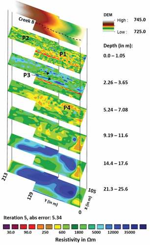
In the layers beneath (from 1.05 to 5.24 m), an area-wide increase of the resistivity values is observed (exceeding 1,500 Ωm), except for the region below Creek B. Here, the resistivity values remain at a low level (<250 Ωm), indicating unfrozen conditions, also in greater depths. It is noticeable that the resistivity rises above 10 kΩm in some areas, especially at depths between 2.26 and 3.65 m. This high resistivity can be interpreted as ice-rich permafrost. However, these are not large-scale, continuous structures but individual separated anomalies elongated in slope direction (P3 in Figure 7). The area in between these high-resistivity anomalies seems to be frozen but has to be considered as less ice-rich as resistivity values range between 1,500 and 3,200 Ωm (i.e., are of lower magnitude). In the depth layer (5.24–7.08 m) as well as in the underlying layer (7.08–9.19 m, not shown), a clear area-wide drop in resistivity to well below 600 Ωm can be seen. According to the low resistivity values, it is assumed that this layer is partially unfrozen and contains a high amount of liquid water. In some parts, the resistivity values drop even below 250 Ωm (P4 in Figure 7). Below a depth of approximately 9 m, there is a slight increase in electrical resistivity again, followed by a sharp increase from about 11.5 m depth downwards. The lower model layers most likely represent ice-rich permafrost or frozen bedrock, because of the resistivity values exceeding more than 10 kΩm.

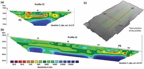
In summary, these results indicate a four-layered structure consisting of the active layer, a partly ice-rich layer of permafrost, an underlying layer of partly unfrozen sediments, and a lowermost high-resistivity layer, most likely representing ice-rich permafrost or frozen bedrock. A detailed discussion of this rather unusual structure follows in the section “Spatiotemporal development and possible relationships to subsurface structure” on this article. The structure is consistent over the entire grid except from the area below the incised Creek B. Here, the low-resistivity surface anomaly continues down to a depth of about 5 m (cf. P1 in Figure 8a). In the longitudinal profile L4 (Figure 8b), it can be seend that the multilayered structure extends along the entire slope. The third layer, represented by lower resistivity values, appears to be frozen over large parts of the profile, because the resistivity values remain above the assumed threshold value. However, the lower slope area starting at 150-m profile length is an exception, because there, at depths between 6 and 10 m, the resistivity values drop below 250 Ωm (P2). The location of the low-resistivity anomaly is striking here, because it lies along the profile in the area closest to the retreating slump headwall. Further, the depth position from 6- to 7-m depth onwards corresponds to the height of the slump headwall and thus also to the approximate depth of the slump floor.

Figure 8. Two 2D electrical resistivity tomography (ERT) profiles of the measured q3D grid. Profile C5 presents a cross-profile measured perpendicular to the slope direction, whereas the longitudinal profile L4 was measured in slope direction. The red lines in the sketch map, which presents all electrode positions on a hillshade map of the unmanned aerial vehicle (UAV)-based digital elevation models (DEM) from 2019, indicate the positions of these profiles. Positions referred to in the text are labeled (P1–P2).

Discussion

Methodological approach

The methodological approach combines a set of remote sensing and geophysical methods to investigate the former and recent development of the RTS. The remote sensing–based analysis of the slump development is based on a simple manual mapping of the slump area using optical satellite data. Only one single image per year could be used for the derivation of yearly spatial changes, because the data availability was low due to the frequent cloud coverage, shading, and rather short snow-free period. Whenever possible, images acquired in late August or early September were chosen, because thaw season is presumed to end in early/mid-September, thus reaching the maximum extent of the slump in a respective year.

The use of UAV-based DEMs for change detection analysis is common in the field of permafrost research (cf. Gaffey and Bhardwaj 2020; Śledź, Ewertowski, and Piekarczyk 2021) and for investigations of RTSs (Armstrong et al. 2018; van der Sluijs et al. 2018; Turner, Pearce, and Hughes 2021). A main problem with this method in permafrost regions is often a lack of stable ground control points due to, for example, permafrost-related surface displacements, vegetation coverage, or missing bedrock outcrops. In this study, prominent positions recognizable in both images were used, and it is assumed that the selected GCPs allowed for a reliable coregistration of the 2018 and 2019 DEMs. Unfortunately, the GCPs could only be measured in the second year, which is why the coregistration of the UAV models was subsequently performed on the basis of these points. The comparison of the two DEMs indicated area-wide changes of less than 5 cm for the (unchanged) vegetated patterns adjacent to the slump. Instead, the vertical and horizontal changes in the area of the slump, related to its development, were between −6.5 and +1.5 m, showing a much higher order of magnitude. The small changes in the undisturbed areas show that at least the internal position accuracy of the two models fits well and the error caused by this is much smaller than the changes to be detected in the area of the slump.

Similar to the use of UAVs, the usage of geophysical methods is common in permafrost research. The application of ERT enables the delineation of frozen and unfrozen areas as well as the derivation of relative ice content changes within the subsurface (Fortier, Allard, and Seguin 1994; Kneisel et al. 2008). The delineation of frozen and unfrozen areas is based on the sharp increase in electrical resistivity at the transition from unfrozen to frozen conditions (Kneisel et al. 2008). Therefore, a threshold value for the delineation should be determined for the site-specific conditions. In the present study, the threshold was set as 600 Ωm based on a cross-check to direct manual frost probing. This threshold is in range detected by other studies in similar arctic and subarctic environments (300–1,000 Ωm; Fortier, Allard, and Seguin 1994; Dobiński 2010; Lewkowicz, Etzelmüller, and Smith 2011; Emmert and Kneisel 2021) but is much lower than in other mountainous regions (Kneisel and Hauck 2008). Varying resistivities within the permafrost highlight small-scale heterogeneity and may be due to different substrates but especially to different ice and water contents in the permafrost. Higher resistivity values point to higher ice contents and lower (pore) water contents within the permafrost (Fortier, Allard, and Seguin 1994; Hauck 2002; Oldenborger and LeBlanc 2018). Whithout drillings, these variations could not be validated in detail, but exposed permafrost at the slump headwall shows distinct heterogeneities in ice content and fits to the detected subsurface structures based on the ERT. The chosen setup with 3-m electrode spacing, up to seventy-two electrodes, and the dipole–dipole array used allowed a detailed and high-resolution investigation of the upper 10 m of the subsurface in the slump environment, which was of particular interest with regard to the slump depth. Further, the chosen interline spacing of 6 m between longitudinal profiles and 12 m between the cross-profiles contributed to the high model resolution of the 3D model. Regardless of the model resolution, the small model error of 5.34 percent (mean absolute error) using the fifth iteration indicates good data quality. Differences between the 2D measurements and the generated 3D model were small and did not affect the interpretation of the results but were in line with findings revealed in previous research (Emmert and Kneisel 2017).

The active layer delineation based on frost probing and GPR delivered area-wide estimates of the ALTs in the area adjacent to the retreating headwall. It should be noted that all measurements were taken in late August and early September close to the end of thaw season. In both years, freeze-back started only few days after the measurements. Nevertheless, it could not be ruled out that the ALT slightly increased during the short period of several days after the measurement. Because the measurements were rounded to an accuracy of 5 cm and the focus of this study was more on spatial heterogeneities than on the temporal ALT development, the mentioned uncertainty was accepted and the detected frost table was interpreted as permafrost table. Both methods are associated with several uncertainties. The manual frost probing results were rounded to an accuracy of 5 cm due to the undefined surface in case of soft vegetation, such as moss cushions and lichens. In addition, the partly coarse-grained material likely did not always allow detecting the permafrost table without doubt. In turn, the GPR results could be calibrated using the frost probing results, but a comparison of the calibrated GPR data and frost probing results showed a poor correlation between the two data sets (Figure 5c). Calibration revealed average signal propagation velocities in the active layer of 0.043 to 0.056 m/ns with decreasing velocity in the downslope direction. In general, these values are in line with values from other studies for a moist active layer in similar environments (Brosten et al. 2009; Kunz and Kneisel 2021) and are also within the theoretical range (Davis and Annan 1989; Moorman, Robinson, and Burgess 2003; Reynolds 2011). However, the calibration enables only a rough approximation due to the small-scale variability in soil moisture. These strong soil moisture variations as well as the inaccuracy in coregistration of the two data sets of approximately 0.5 m affects the correlation of the two data sets. The mentioned velocity decrease in the downslope direction is possibly due to an increase in soil moisture downslope and ensures that the time–depth conversion in the slope-parallel profiles could not be performed with a single standard value. Instead, the average velocity was calculated for each profile covered by GPR and frost probing and the propagation velocity of the closest calibrated profile was used for the intervening GPR profiles. The mentioned inaccuracies in the methodological approaches to localize the permafrost table also affect the hydrological modeling results based on these data. The permafrost table model derived from frost probing is comparatively coarse-scaled. The distance between the original data points was 6 m and, therefore, much higher than in the GPR-derived data set. The GPR-derived permafrost table model is much more detailed and the resulting hydrological data look much more heterogenous. This heterogeneity is more in line with the actual small-scale variability of both ALTs and permafrost table topography, also proven by digging, although the absolute values do not show a good correlation.

Overall, the combined methodological approach allowed a comprehensive investigation of the slump environment in terms of subsurface structures and permafrost hydrology, as well as the spatiotemporal evolution of the RTS.

Spatiotemporal development and possible relationships to subsurface structure

The initialization of the slump likely originated from a small stream channel (Creek A) and is therefore likely due to erosion of the insulating active layer in the riparian area. This is considered a typical origin of RTSs (French 2017). The slump was first detected in summer 2014 in the remote sensing imagery with a rather small area of approximately 160 m². Nevertheless, the initial rupture of the slump in the riparian area of the creek could already have occurred some years before. It is possible that increased precipitation, and possibly higher ALTs, caused increased erosion in the streambed, which in turn contributed to the initialization or reactivation of the slump. The expected runoff volumes for the RTS under investigation might be comparatively low, considering the rather small size of the catchment (2.16 ha). However, the runoff is further influenced by thermal erosion in the slightly incised streambed and is therefore dynamic in nature.

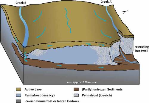
Permafrost table topography affects the local hydrology due to a canalization of water on top of the permafrost table. The detected furrows, revealed by GPR and frost probing and also visible in the soil pit (Figure 1d), concentrate the runoff in the downslope direction and in some parts toward the slump. This is highlighted by the hydrological modeling and is indicated in a simplified model of the subsurface structures in Figure 9. Furthermore, the subsurface structures detected by ERT could have a strong influence on the hydrology. Especially the partially unfrozen layer at a depth of about 6 to 10 m could be directly connected to the slump floor because the anomaly continues also in the profiles closest to the slump. This low-resistivity layer could therefore represent a possible water pathway, potentially providing an underground connection between Creek B in the southwest of the grid and the slump floor. A possible connection to Creek B further upslope is also supported by the 2D profiles. At the profile position of approximately 35 m in profile C5 (Figure 8), it can be seen that there is a small intersection (green, P1) of the low-resistivity structure (yellow and brownish) at a depth between 6 and 7 m below the surface. Nevertheless, the intersection area is also characterized by resistivity values close to 600 Ωm and, therefore, close to the assumed threshold value between frozen and unfrozen ground. Hence, the unfrozen layer provides a potential connection between the creek and the slump floor that may affect the hydrology. The formation of a talik at this depth is rather atypical but could be related to the detected talik below the creeks. These might affect subsurface hydrology and thus cause a thermal impact also at greater depths. This impact could have propagated along flow paths and thus contributed to the formation of this partly unfrozen layer. The subsurface structure including this layer and possible water pathways are shown in the simplified block model in Figure 9. This detected subsurface structure fits to the observations of other studies where comparatively warm permafrost temperatures (−1°C to −3°C) were measured (O’Neill et al. 2015), and icing events were detected in this region (Crites, Kokelj, and Lacelle 2020), indicating water pathways and occurrences within the permafrost. The partly unfrozen layer also affects the slump development and represents a kind of lower limit for the slump headwall due to the rather low ice content or even the absence of ice. This layer would not be affected or only slightly affected by permafrost thaw and ground ice melt and therefore would probably not be subject to such rapid erosion as the overlying ice-rich layer.

Figure 9. Simplified illustration of the detected subsurface structures as well as derived water pathways (blue arrows). The figure is not drawn to scale and is shown vertically exaggerated.

Within the frozen layer, the ERT measurements also revealed varying ice contents, which were also visible at the exposed slump headwall. In some areas, nearly pure ice was exposed at the headwall, whereas in other parts frozen sediment without visible ice lenses was exposed. A comparison of the observations with the ERT results supports the interpretations, because the areas where high resistivities were detected were in close proximity to the areas where high ice contents or massive ice were visible in the headwall. This varying ice content may also affect the spatial development of the slump. Whereas the slump extends especially in a southern and southwestern direction during the first years, it has expanded in a western and northwestern direction since 2018. This is possibly due to lower ice content in the area south of the slump, whereas higher electrical resistivities were measured in the area to the west adjacent to the slump, indicating a higher ice content. Erosion is therefore progressing toward areas characterized by higher ice content (cf. Lewkowicz 1987) and would thus be directly influenced by subsurface properties as already assumed in previous studies (e.g., Lewkowicz 1987; Lacelle et al. 2015; Bernhard et al. 2022; Hayes et al. 2022). This suspicion was also confirmed by comparison with an ERT reconnaissance profile surveyed in August 2018 that was measured along the headwall diagonally across the slope. The profile showed higher resistivity values in the area west of the slump, whereas the resistivity values south and southwest of the slump indicated low ice contents or partly unfrozen conditions. Erosion up to the 2019 measurements then occurred in exactly those areas where high electrical resistivities, and thus high ice contents, were detected in 2018. In the direction of the areas that had lower resistivity values, no or only minor expansion of the slump took place. This suggests that in addition to hydrology and general relief characteristics, subsurface properties (in particular ice content) have a distinct influence on spatiotemporal slump development.

Other RTSs in the region typically show an eastern exposure of the slope (cf. Lacelle et al. 2015; Bernhard et al. 2022). The RTS investigated in this study shows a slope with southeastern orientation. It should be noted that the slump was initiated in the northeast-exposed riparian area of the creek and subsequently extended toward the south and west. The elevation of the slump is close to the uppermost limit of RTSs in the region, which is due to the expected limited distribution of ice-rich permafrost or massive ground ice up to an elevation of 750 m.a.s.l. This distribution is closely related to the outermost limit of the LIS (Lacelle et al. 2013, 2015). The size of the slump (approximately 6,000 m²), its annual increase in thawed area, and the volume of material eroded annually were lower than the regional average and were in the lower limit of the regional spectrum. Nevertheless, based on the UAV surveys conducted in 2018 and 2019, an area-to-volume scaling factor of 1.285 can be determined from the annual change in thawed area (891 m²) and the thawed volume eroded during the same period (6,170 m³). This value describes the scaling exponent of the power law relationship between the disturbed area and the volumetric change. A similar value (1.27) was calculated as regional average (from 438 RTSs) by Bernhard et al. (2022) for the Peel Plateau region, whereas S. V. Kokelj et al. (2021) calculated a distinctly higher average scaling factor (1.42) for seventy-one slumps in the Peel Plateau, the Anderson Plain, and the Tuktoyaktuk Coastland region. However, the scaling factors were calculated in different ways in these studies. Whereas S. V. Kokelj et al. (2021) calculated the factor using the entire slump scar volume and area, Bernhard et al. (2022) used a simplified approach using calculated annual area and volume changes derived from headwall retreat. We also used the simplified approach and thus only the changes in area and volume but were able to use very high-resolution data to calculate these parameters. A more precise calculation would need a predisturbance relief data set as recommended by van der Sluijs, Kokelj, and Tunnicliffe (2022).

The influence on downstream areas is likely rather small due to the comparatively small size. As mentioned above, the material was mostly redeposited in the direct vicinity of the headwall and only a very small part was transported away via the headwaters. Nevertheless, the occurrence of RTSs also affects the water chemistry. Therefore, a certain influence on the downstream waters is still to be expected at the investigated RTS. A geochemical analysis of samples from the headwall, debris, and runoff conducted by Bröder et al. (2021) showed that the slump did not differ significantly from other slumps in the vicinity regarding different geochemical parameters. The redeposition of the eroded material (cf. Figure 2) led to a rise of the slump floor level and a relative decrease in the headwall height. In the long run, accumulation in the slump floor area could potentially lead to a stabilization of the slump so that, similar to the adjacent slump scar, no more material is removed. This would also fit with observations at other slumps in the Mackenzie Delta region that demonstrated a positive relationship between headwall height and erosion rates (B. Wang, Paudel, and Li 2016). A decreasing headwall height would therefore also indirectly indicate a decreasing erosion rate and support the stabilization (S. V. Kokelj et al. 2015).

Conclusion

The presented study employs a multimethod approach to investigate the past and present development of a retrogressive thaw slump and to characterize subsurface structures in regions adjacent to the retreating headwall. The analysis of high-resolution satellite data evidenced the initialization of the slump in summer 2014 at the latest and an increasing growth of the retrogressive thaw slump since then. In particular, annual growth rates have increased significantly since the summer of 2018, when the slump also started to expand toward a local creek. By means of two UAV-based digital elevation models, a horizontal retreat of the headwall between 4 and 11 m was detected during the period August 2018 to August 2019. A simultaneous accumulation of eroded material in the slump floor led to its rise and thus to a decrease in the headwall height from 7.5 to 6.5 m. A clear relationship between the ALTs and the relief position in the vicinity of the slump could be identified employing manual frost probing and at least partially by GPR surveying. In addition, GPR revealed material sorting within the active layer affecting the ALTs and the local hydrology. In combination with the varying ALTs, it caused a canalization of water on top of the permafrost table. By means of q3D electrical resistivity tomography, a heterogeneous layer of ice-rich permafrost was detected, which was underlain by a very low-resistivity (probably partially unfrozen) layer at a depth of about 6 to 10 m. This layer represents a possible water pathway within the permafrost body and possibly forms a connection to an unfrozen area below an adjacent creek. A comparison of the slump development with the detected subsurface structures indicated that the spatial development of the slump was affected not only by hydrological and relief-related parameters but also by the subsurface structures and in particular by the ice content. However, the spatial and temporal development of the slump must be further investigated to make more precise statements in this regard.

To the authors’ knowledge, this is the first study conducting a detailed 3D investigation of subsurface structures adjacent to an active slump headwall. Previous studies have mostly relied on drillings, but these cannot detect the observed heterogeneities to this extent. To gain further insight into the interactions between subsurface structures and slump development, the approach would be useful to transfer the approach to other slumps in the region and combine it with drillings as absolute validation. Especially in the context of accelerated climate warming, this could help to better understand the complex interactions in RTSs and to better predict their future development.

Acknowledgments

We thank the Education and Research Program by Planet Lab for providing free access to PlanetScope satellite imagery for scientific purposes and Sebastian Buchelt for data aquisition. We are grateful to Franziska Losert, Blair Kennedy, Andreas Bury, Leon Nill, and Tim Wiegand for their untiring support in the field. Thanks also to the Northwest Territories for the issued research permits and Aurora Research Institute (Inuvik, NWT, Canada) and K&K TruckRentals (Whitehorse, YT, Canada) for logistical support. We also thank the two reviewers for their constructive and fair reviews, which contributed to a significant improvement of the article.

Disclosure statement

No potential conflict of interest was reported by the authors.

Additional information

Funding

This study was funded by the German Research Foundation (DFG 329721376). The Digital Elevation Model of the TanDEM-X Mission is shown under the permission of the German Aerospace Center (DLR), Germany, ©DLR, 2016 (proposal “IDEM_HYDRO0182” and TanDEM-X Science proposal “DEM_OTHER1323”). This publication was supported by the Open Access Publication Fund of the University of Wuerzburg.

References

- AgiSoft PhotoScan Professional. 2016. Version 1.2.6. (Software). St. Petersburg, Russia. http://www.agisoft.com/downloads/installer/.
- Armstrong, L., D. Lacelle, R. H. Fraser, S. Kokelj, and A. Knudby. 2018. Thaw slump activity measured using stationary cameras in time-lapse and structure-from-motion photogrammetry. Arctic Science 4 (4):827–19. doi:10.1139/as-2018-0016.
- Bailey, P., J. Wheaton, M. Reimer, and J. Brasington. 2020. Geomorphic Change Detection 7 (Version 7.5.0.0) (Software). doi: 10.5281/zenodo.7248344.
- Balser, A. W. 2015. Retrogressive thaw slumps and active layer detachment slides in the Brooks Range and Foothills of northern Alaska: Terrain and timing. Fairbanks: University of Alaska, Fairbanks. doi:10.13140/RG.2.1.4497.6160.
- Balser, A. W., J. B. Jones, and R. Gens. 2014. Timing of retrogressive thaw slump initiation in the Noatak Basin, northwest Alaska, USA. Journal of Geophysical Research: Earth Surface 119 (5):1106–20. doi:10.1002/2013JF002889.
- Bernhard, P., S. Zwieback, N. Bergner, and I. Hajnsek. 2022. Assessing volumetric change distributions and scaling relations of retrogressive thaw slumps across the Arctic. The Cryosphere 16 (1):1–15. doi:10.5194/tc-16-1-2022.
- Böhner, J., R. Koethe, O. Conrad, J. Gross, A. Ringeler, and T. Selige. 2002. Soil regionalisation by means of terrain analysis and process parameterisation. In Soil Classification 2001, ed. E. Micheli, F. O. Nachtergaele, R. J. A. Jones and L. Montanarella, 248. Luxembourg: Office for Official Publications of the European Communities.
- Bröder, L., K. Keskitalo, S. Zolkos, S. Shakil, S. E. Tank, S. V. Kokelj, T. Tesi, B. E. Van Dongen, N. Haghipour, T. I. Eglinton, et al. 2021. Preferential export of permafrost-derived organic matter as retrogressive thaw slumping intensifies. Environmental Research Letters 16 (5):054059. doi:10.1088/1748-9326/abee4b.
- Brooker, A., R. H. Fraser, I. Olthof, S. V. Kokelj, and D. Lacelle. 2014. Mapping the activity and evolution of retrogressive thaw slumps by tasselled cap trend analysis of a Landsat satellite image stack: Evolution of thaw slumps based on tasselled cap trend analysis. Permafrost and Periglacial Processes 25 (4):243–56. doi:10.1002/ppp.1819.
- Brosten, T. R., J. H. Bradford, J. P. McNamara, M. N. Gooseff, J. P. Zarnetske, W. B. Bowden, and M. E. Johnston. 2009. Estimating 3D variation in active-layer thickness beneath Arctic streams using ground-penetrating radar. Journal of Hydrology 373 (3–4):479–86. doi:10.1016/j.jhydrol.2009.05.011.
- Brown, J., F. J. Sidlauskas, and G. Delinski. 1997. Circum-Arctic map of permafrost and ground ice conditions [Map]. The Survey; For sale by Information Services.
- Campbell, S. W., M. Briggs, S. G. Roy, T. A. Douglas, and S. Saari. 2021. Ground‐penetrating radar, electromagnetic induction, terrain, and vegetation observations coupled with machine learning to map permafrost distribution at Twelvemile Lake, Alaska. Permafrost and Periglacial Processes 32 (3):407–26. doi:10.1002/ppp.2100.
- Chen, A., A. D. Parsekian, K. Schaefer, E. Jafarov, S. Panda, L. Liu, T. Zhang, and H. Zebker. 2016. Ground-penetrating radar-derived measurements of active-layer thickness on the landscape scale with sparse calibration at Toolik and Happy Valley, Alaska. Geophysics 81 (2):H9–H19. doi:10.1190/geo2015-0124.1.
- Conrad, O., B. Bechtel, M. Bock, H. Dietrich, E. Fischer, L. Gerlitz, J. Wehberg, V. Wichmann, and J. Böhner. 2015. System for Automated Geoscientific Analyses (SAGA) v. 2.1.4. Geoscientific Model Development 8 (7):1991–2007. doi:10.5194/gmd-8-1991-2015.
- Crites, H., S. V. Kokelj, and D. Lacelle. 2020. Icings and groundwater conditions in permafrost catchments of northwestern Canada. Scientific Reports 10 (1):3283. doi:10.1038/s41598-020-60322-w.
- Davis, J. L., and A. P. Annan. 1989. Ground-penetrating radar for high-resolution mapping of soil and rock stratigraphy. Geophysical Prospecting 37 (5):531–51. doi:10.1111/j.1365-2478.1989.tb02221.x.
- Dobiński, W. 2010. Geophysical characteristics of permafrost in the Abisko area, northern Sweden. Polish Polar Research 31 (2):141–58. doi:10.4202/ppres.2010.08.
- Duk-Rodkin, A. 1992. Surficial geology, Fort McPherson-Bell River, Yukon-Northwest Territories. [Map]. Geological Survey of Canada, Ottawa. doi:10.4095/184002
- Emmert, A., and C. Kneisel. 2017. Internal structure of two alpine rock glaciers investigated by quasi-3-D electrical resistivity imaging. The Cryosphere 11 (2):841–55. doi:10.5194/tc-11-841-2017.
- Emmert, A., and C. Kneisel. 2021. Internal structure and palsa development at Orravatnsrústir Palsa site (Central Iceland), investigated by means of integrated resistivity and ground‐penetrating radar methods. Permafrost and Periglacial Processes 32 (3):503–19. doi:10.1002/ppp.2106.
- ESRI Inc. 2018. ArcGis Desktop - ArcMap Version 10.6.1 (Software). Redlands, CA. https://www.esri.com/.
- Fortier, R., M. Allard, and M.-K. Seguin. 1994. Effect of physical properties of frozen ground on electrical resistivity logging. Cold Regions Science and Technology 22 (4):361–84. doi:10.1016/0165-232X(94)90021-3.
- Fraser, R., I. Olthof, S. Kokelj, T. Lantz, D. Lacelle, A. Brooker, S. Wolfe, and S. Schwarz. 2014. Detecting landscape changes in high latitude environments using Landsat trend analysis: 1. Visualization. Remote Sensing 6 (11):11533–57. doi:10.3390/rs61111533.
- French, H. M. (2017). The periglacial environment. 4th ed. Chichester: John Wiley & Sons, Ltd. 10.1002/9781119132820.
- French, H. M., and P. Egginton. 1973. Thermokarst Development, Banks Island, Western Canadian Arctic. In Permafrost: North American Contribution to the Second International Conference, 203–212. Washington: National Academy of Sciences.
- Gaffey, C., and A. Bhardwaj. 2020. Applications of unmanned aerial vehicles in cryosphere: Latest advances and prospects. Remote Sensing 12 (6):948. doi:10.3390/rs12060948.
- Geotomo Software SDN BHD. 2015. RES2DINVx64 (Version 4.05.41) (Software). Gelugor, Malaysia. http://geotomosoft.com.
- Geotomo Software SDN BHD. 2016. RES3DINVx64 (Version 3.11.73) (Software). Gelugor, Malaysia. http://geotomosoft.com.
- Government of Canada. 2020. Canadian climate normals 1981-2010 station data—Fort McPherson A. https://climate.weather.gc.ca/climate_normals/results_1981_2010_e.html?searchType=stnName&txtStationName=Fort+McPherson&searchMethod=contains&txtCentralLatMin=0&txtCentralLatSec=0&txtCentralLongMin=0&txtCentralLongSec=0&stnID=1648&dispBack=1. December 10.
- Gruber, S., and S. Peckham. 2009. Chapter 7: Land-Surface Parameters and Objects in Hydrology. In Geomorphometry - Concepts, Software, Applications. Developments in Soil Science, ed. T. Hengl and T. I. Reuter. Vol. 33, 171–94. Amsterdam: Elsevier. doi: 10.1016/S0166-2481(08)00007-X.
- Hauck, C. 2002. Frozen ground monitoring using DC resistivity tomography. Geophysical Research Letters 29 (21):2016. doi:10.1029/2002GL014995.
- Hauck, C. 2013. New concepts in geophysical surveying and data interpretation for permafrost terrain: Geophysical surveying in permafrost terrain. Permafrost and Periglacial Processes 24 (2):131–37. doi:10.1002/ppp.1774.
- Hayes, S., M. Lim, D. Whalen, P. J. Mann, P. Fraser, R. Penlington, and J. Martin. 2022. The role of massive ice and exposed headwall properties on retrogressive thaw slump activity. Journal of Geophysical Research: Earth Surface 127:e2022JF006602. doi:10.1029/2022JF006602.
- Henry, K., and M. Smith. 2001. A model-based map of ground temperatures for the permafrost regions of Canada. Permafrost and Periglacial Processes 12 (4):389–98. doi:10.1002/ppp.399.
- Hinkel, K. M., J. A. Doolittle, J. G. Bockheim, F. E. Nelson, R. Paetzold, J. M. Kimble, and R. Travis. 2001. Detection of subsurface permafrost features with ground-penetrating radar, Barrow, Alaska. Permafrost and Periglacial Processes 12 (2):179–90. doi:10.1002/ppp.369.
- Intergovernmental Panel on Climate Change. 2021. Climate Change 2021: The Physical Science Basis. Contribution of Working Group I to the Sixth Assessment Report of the Intergovernmental Panel on Climate Change.
- Kneisel, C., C. Hauck, R. Fortier, and B. Moorman. 2008. Advances in geophysical methods for permafrost investigations. Permafrost and Periglacial Processes 19 (2):157–78. doi:10.1002/ppp.616.
- Kneisel, C., C. Hauck. 2008. Electrical methods. In ed. C. Hauck and C. Kneisel, Applied geophysics in periglacial environments, 3–27. Cambridge: Cambridge University Press. doi:10.1017/CBO9780511535628.002.
- Kokelj, S. A., C. R. Beel, R. F. Connon, C. E. D. Graydon, S. V. Kokelj, and C. R. Burn. 2022. Peel Plateau climate data, Northwest Territories. NWT Open Report 2022-005. doi:10.46887/2022-005
- Kokelj, S. V., J. Kokoszka, J. van der Sluijs, A. C. A. Rudy, J. Tunnicliffe, S. Shakil, S. E. Tank, and S. Zolkos. 2021. Thaw-driven mass wasting couples slopes with downstream systems, and effects propagate through Arctic drainage networks. The Cryosphere 15 (7):3059–81. doi:10.5194/tc-15-3059-2021.
- Kokelj, S. V., D. Lacelle, T. C. Lantz, J. Tunnicliffe, L. Malone, I. D. Clark, and K. S. Chin. 2013. Thawing of massive ground ice in mega slumps drives increases in stream sediment and solute flux across a range of watershed scales. Journal of Geophysical Research: Earth Surface 118 (2):681–92. doi:10.1002/jgrf.20063.
- Kokelj, S. V., J. Tunnicliffe, D. Lacelle, T. C. Lantz, K. S. Chin, and R. Fraser. 2015. Increased precipitation drives mega slump development and destabilization of ice-rich permafrost terrain, northwestern Canada. Global and Planetary Change 129:56–68. doi:10.1016/j.gloplacha.2015.02.008.
- Kunz, J., and C. Kneisel. 2021. Three‐dimensional investigation of an open‐ and a closed‐system Pingo in northwestern Canada. Permafrost and Periglacial Processes 32 (4):541–57. doi:10.1002/ppp.2115.
- Lacelle, D., A. Brooker, R. H. Fraser, and S. V. Kokelj. 2015. Distribution and growth of thaw slumps in the Richardson Mountains–Peel Plateau region, northwestern Canada. Geomorphology 235:40–51. doi:10.1016/j.geomorph.2015.01.024.
- Lacelle, D., B. Lauriol, G. Zazula, B. Ghaleb, N. Utting, and I. D. Clark. 2013. Timing of advance and basal condition of the Laurentide Ice Sheet during the Last Glacial Maximum in the Richardson Mountains, NWT. Quaternary Research 80 (2):274–83. doi:10.1016/j.yqres.2013.06.001.
- Lantuit, H., and W. H. Pollard. 2008. Fifty years of coastal erosion and retrogressive thaw slump activity on Herschel Island, southern Beaufort Sea, Yukon Territory, Canada. Geomorphology 95 (1–2):84–102. doi:10.1016/j.geomorph.2006.07.040.
- Lewkowicz, A. G. 1987. Headwall retreat of ground-ice slumps, Banks Island, Northwest Territories. Canadian Journal of Earth Sciences 24 (6):1077–85. doi:10.1139/e87-105.
- Lewkowicz, A. G., B. Etzelmüller, and S. L. Smith. 2011. Characteristics of discontinuous permafrost based on ground temperature measurements and electrical resistivity tomography, Southern Yukon, Canada. Permafrost and Periglacial Processes 22 (4):320–42. doi:10.1002/ppp.703.
- Lewkowicz, A. G., and R. G. Way. 2019. Extremes of summer climate trigger thousands of thermokarst landslides in a High Arctic environment. Nature Communications 10 (1):1329. doi:10.1038/s41467-019-09314-7.
- Littlefair, C. A., S. E. Tank, and S. V. Kokelj. 2017. Retrogressive thaw slumps temper dissolved organic carbon delivery to streams of the Peel Plateau, NWT, Canada. Biogeosciences 14 (23):5487–505. doi:10.5194/bg-14-5487-2017.
- Loke, M. H. 2019. Rapid 3-D Resistivity & IP inversion using the least-squares method (For 3-D surveys using the pole-pole, pole-dipole, dipole-dipole, rectangular, Wenner, Wenner-Schlumberger, vector and non-conventional arrays) on land, aquatic, cross-borehole and time-lapse surveys.
- Mackay, J. R. 1967. Permafrost depths, Lower Mackenzie Valley, Northwest Territories. Arctic, 21–26.
- Moorman, B. J., S. D. Robinson, and M. M. Burgess. 2003. Imaging periglacial conditions with ground-penetrating radar. Permafrost and Periglacial Processes 14 (4):319–29. doi:10.1002/ppp.463.
- Munroe, J. S., J. A. Doolittle, M. Z. Kanevskiy, K. M. Hinkel, F. E. Nelson, B. M. Jones, Y. Shur, and J. M. Kimble. 2007. Application of ground-penetrating radar imagery for three-dimensional visualisation of near-surface structures in ice-rich permafrost, Barrow, Alaska. Permafrost and Periglacial Processes 18 (4):309–21. doi:10.1002/ppp.594.
- Nill, L., I. Grünberg, T. Ullmann, M. Gessner, J. Boike, and P. Hostert. 2022. Arctic shrub expansion revealed by Landsat-derived multitemporal vegetation cover fractions in the Western Canadian Arctic. Remote Sensing of Environment 281:113228. doi:10.1016/j.rse.2022.113228.
- Nill, L., T. Ullmann, C. Kneisel, J. Sobiech-Wolf, and R. Baumhauer. 2019. Assessing Spatiotemporal Variations of Landsat land surface temperature and multispectral indices in the Arctic Mackenzie Delta Region between 1985 and 2018. Remote Sensing 11 (19):2329. doi:10.3390/rs11192329.
- Nitze, I., K. Heidler, S. Barth, and G. Grosse. 2021. Developing and testing a deep learning approach for mapping retrogressive thaw slumps. Remote Sensing 13 (21):4294. doi:10.3390/rs13214294.
- Oldenborger, G. A., and A.-M. LeBlanc. 2018. Monitoring changes in unfrozen water content with electrical resistivity surveys in cold continuous permafrost. Geophysical Journal International 215 (2):965–77. doi:10.1093/gji/ggy321.
- O’Neill, H. B., C. R. Burn, S. V. Kokelj, and T. C. Lantz. 2015. ‘Warm’ tundra: Atmospheric and near-surface ground temperature inversions across an alpine treeline in continuous permafrost, Western Arctic, Canada: Near-surface ground temperatures across an alpine treeline. Permafrost and Periglacial Processes 26 (2):103–18. doi:10.1002/ppp.1838.
- O’Neill, H. B., S. A. Wolfe, and C. Duchesne. 2022. Ground ice map of Canada (No. 8713; version 1.1, p. 8713). San Francisco, CA: Planet Labs PBC. doi:10.4095/330294.
- Planet Labs PBC. San Francisco, CA. https://www.planet.com
- Ramage, J. L., A. M. Irrgang, U. Herzschuh, A. Morgenstern, N. Couture, and H. Lantuit. 2017. Terrain controls on the occurrence of coastal retrogressive thaw slumps along the Yukon Coast, Canada: Coastal RTSs along the Yukon Coast. Journal of Geophysical Research: Earth Surface 122 (9):1619–34. doi:10.1002/2017JF004231.
- Reynolds, J. M. 2011. An introduction to applied and environmental geophysics. 2nd ed. Chichester: Wiley-Blackwell.
- Rödder, T., and C. Kneisel. 2012. Permafrost mapping using quasi-3D resistivity imaging, Murtèl, Swiss Alps. Near Surface Geophysics 10 (2):117–27. doi:10.3997/1873-0604.2011029.
- Segal, R. A., T. C. Lantz, and S. V. Kokelj. 2016. Acceleration of thaw slump activity in glaciated landscapes of the Western Canadian Arctic. Environmental Research Letters 11 (3):034025. doi:10.1088/1748-9326/11/3/034025.
- Shakil, S., S. E. Tank, S. V. Kokelj, J. E. Vonk, and S. Zolkos. 2020. Particulate dominance of organic carbon mobilization from thaw slumps on the Peel Plateau, NT: Quantification and implications for stream systems and permafrost carbon release. Environmental Research Letters 15 (11):114019. doi:10.1088/1748-9326/abac36.
- Śledź, S., M. W. Ewertowski, and J. Piekarczyk. 2021. Applications of unmanned aerial vehicle (UAV) surveys and structure from motion photogrammetry in glacial and periglacial geomorphology. Geomorphology 378:107620. doi:10.1016/j.geomorph.2021.107620.
- Smith, C. A. S., J. C. Meikle, and C. F. Roots (eds.). 2004. Ecoregions of the Yukon Territory: Biophysical properties of Yukon landscapes. Agriculture and Agri-Food Canada. PARC Technical Bulletin No. 04-01, Summerland, British Columbia, 313.
- Swanson, D., and M. Nolan. 2018. Growth of retrogressive thaw slumps in the Noatak Valley, Alaska, 2010–2016, measured by airborne photogrammetry. Remote Sensing 10 (7):983. doi:10.3390/rs10070983.
- Turner, K. W., M. D. Pearce, and D. D. Hughes. 2021. Detailed characterization and monitoring of a retrogressive thaw slump from remotely piloted aircraft systems and identifying associated influence on carbon and nitrogen export. Remote Sensing 13 (2):171. doi:10.3390/rs13020171.
- van der Sluijs, J., S. Kokelj, R. Fraser, J. Tunnicliffe, and D. Lacelle. 2018. Permafrost terrain dynamics and infrastructure impacts revealed by UAV photogrammetry and thermal imaging. Remote Sensing 10 (11):1734. doi:10.3390/rs10111734.
- van der Sluijs, J., S. V. Kokelj, and J. F. Tunnicliffe. 2022. Allometric scaling of retrogressive thaw slumps [Preprint]. The Cryosphere Discussions. doi:10.5194/tc-2022-149.
- Wang, L., and H. Liu. 2006. An efficient method for identifying and filling surface depressions in digital elevation models for hydrologic analysis and modelling. International Journal of Geographical Information Science 20 (2):193–213. doi:10.1080/13658810500433453.
- Wang, B., B. Paudel, and H. Li. 2016. Behaviour of retrogressive thaw slumps in northern Canada—Three-year monitoring results from 18 sites. Landslides 13 (1):1–8. doi:10.1007/s10346-014-0549-y.
- Ward Jones, M. K., W. H. Pollard, and B. M. Jones. 2019. Rapid initialization of retrogressive thaw slumps in the Canadian high Arctic and their response to climate and terrain factors. Environmental Research Letters 14 (5):055006. doi:10.1088/1748-9326/ab12fd.
- Wheaton, J. M. 2008. Uncertainity in morphological sediment budgeting of rivers. Southampton: University of Southampton.
- Wheaton, J. M., J. Brasington, S. E. Darby, J. Merz, G. B. Pasternack, D. Sear, and D. Vericat. 2010. Linking geomorphic changes to salmonid habitat at a scale relevant to fish. River Research and Applications 26 (4):469–86. doi:10.1002/rra.1305.
- Wheaton, J. M., J. Brasington, S. E. Darby, and D. A. Sear. 2010. Accounting for uncertainty in DEMs from repeat topographic surveys: Improved sediment budgets. Earth Surface Processes and Landforms 35 (2):136–56. doi:10.1002/esp.1886.
- Wheeler, J. O., P. F. Hoffman, K. D. Card, A. Davidson, B. V. Sanford, A. V. Okulitch, and W. R. Roest. 1996. Geological map of Canada [Map]. doi:10.4095/208175
- Yukon Geological Survey. 2020. Yukon digital bedrock geology [Map]. https://data.geology.gov.yk.ca/Compilation/3
- Zolkos, S., S. E. Tank, R. G. Striegl, S. V. Kokelj, J. Kokoszka, C. Estop-Aragonés, and D. Olefeldt. 2020. Thermokarst amplifies fluvial inorganic carbon cycling and export across watershed scales on the Peel Plateau, Canada. Biogeosciences 17 (20):5163–82. doi:10.5194/bg-17-5163-2020.