Heat balance of a low-elevated Svalbard glacier during the ablation season: A case study of Aldegondabreen

ABSTRACT

On the basis of in situ weather observations and a physical-based model, verified by a glaciological method, this article investigates the surface energy balance of the Aldegondabreen glacier during the summer melt season of 2021. Aldegondabreen (5.3 km²) is a low-elevation glacier near the western shore of Spitsbergen Island. On the timescale of the whole melt season, the prevalent positive heat flux is a shortwave radiative balance (84 percent). This result is in accordance with previous studies on similar low-elevation Svalbard glaciers. However, in August and September, when the sun is low, the turbulent fluxes may outweigh the input of the shortwave balance. The study identified six events of significantly increased turbulent fluxes, which contributed to 10 percent of the total heat influx, and attributed them to the particular type of synoptic situation. All of these events are related to cyclonic activity, which drastically increased the wind speed in the study area and, consequently, both sensible and latent heat fluxes. The frequency of the extreme cyclonic events in the Svalbard region is increasing, which may potentially extend the duration of the glacier melt season in the mid- and late autumn or reduce the accumulation of solid precipitation in that time period.

KEYWORDS:

• Svalbard
• glacier
• ablation
• heat balance
• physical modeling

Introduction

The Svalbard archipelago is covered with 33,775 km² of glaciers, whose volume corresponds to a sea level equivalent of 1.5 cm (Nuth et al. 2013; Schuler et al. 2020). Compared to other glaciated areas in the High Arctic, Svalbard is markedly less elevated (Noël et al. 2020). The peak of its hypsometry is at 300 to 550 m above sea level, and it coincides with the present-day archipelago-averaged equilibrium-line altitude (ELA). In recent decades, a negative mass balance trend has been observed, which is linked to a pronounced atmospheric warming (Van Pelt et al. 2019).

The energy budget and the mechanisms of glacier melt on Svalbard are well studied. Aas et al. (2016) showed that the radiative balance is the main contributor to Svalbard glacier melt in interannual variability, whereas sensible and latent heat fluxes make a significant contribution in years with the most melt. Larger ice masses comprising major ice caps and inland ice fields, located well above the ELA, still possess an extensive accumulation zone and their mean albedo is relatively high throughout the year, making them less vulnerable to downwelling solar radiation (Van Pelt, Pohjola, and Reijmer 2016). However, for some high-lying glaciers, despite the large temperature change gradient and negative latent heat flux values, the ratio of heat balance components is contributed 90 percent by solar radiation and 10 percent by sensible heat flux (Małecki 2015). Several studies (Möller et al. 2011; Østby et al. 2013) indicated the significant contribution of refreezing to the Svalbard glacier surface energy and mass balance. Porous and cold firn and snow layers may act as a buffer to retain the meltwater, decreasing the mass loss and refreezing liquid precipitation (Łupikasza et al. 2019).

However, a number of much smaller and lower-elevation glaciers are present within Spitsbergen: the central parts of the island are dominated by small cirque and valley glaciers (Möller and Kohler 2018). Here the glaciation is retreating faster and is now below ELA (Chernov et al. 2019). The energy fluxes on these glaciers and the topographic controls on them were described in Arnold et al. (2006) and Zou et al. (2021) using case studies of Midtre and Austre Lovénbreen near the town of Ny-Ålesund. One of the main outcomes was that solar radiation was the dominant component in a surface heat balance of a low-elevation glaciers, in contrast to the turbulent fluxes.

In the vicinity of Barentsburg, heat balance studies on the glaciers are rather episodic. Prokhorova et al. (2021) estimated that turbulent fluxes were one magnitude less than the shortwave balance for Aldegondabreen during the ablation season of 2019. This study was significantly limited in time, lasting only for August, and the used model had some major constraints: the constant zero temperature of the ice surface and negligible conductive heat flux were assumed. The heat balance measurement series around Barentsburg in the second half of the twentieth century was summarized in Troitsky et al. (1975). The conclusion was that the turbulent fluxes supplied up to 50 percent of heat available for a glacier melt, which is now considered unlikely.

However, in this study, we focus on the question of which weather events are able to dramatically amplify the turbulent heat fluxes and to what extent. Heat balance modeling, which the authors rely on, is helpful to understand the surface–atmosphere interaction processes in the cryosphere as a physically based approach (Hock 2005). First, the article presents the results of the distributed heat balance model for the whole melt season of May to September 2021, verified with direct ice ablation measurements. Then we identify and discuss the nature of all events of increased turbulent heat fluxes, which were observed during the summer season, to suggest reasonable projections in case these events are likely to increase in frequency in the near future.

Materials and methods

Study site

Aldegondabreen glacier is a mountain–valley glacier located in the western part of Nordenskiöld Land of Spitsbergen island, around 10 km from the town of Barentsburg. Since the end of the Little Ice Age, which occurred on Svalbard in the beginning of the twentieth century (Strzelecki et al. 2018), when Aldegondabreen was a tidewater glacier, it has decreased five times in volume and halved in length (Holmlund 2021). The glacier area is currently around 5.3 km² (Borisik et al. 2021). Almost the whole glacier surface is located below 500 m.a.s.l., making it lower than the present-day snowline on Svalbard (Noël et al. 2020).

In situ ice ablation measurements

The surface mass balance was measured annually using a farm of fourteen wooden stakes (Figure 1a). The stakes were distributed to cover all of the 50-m elevation bins and used to compute the area-averaged mass balance using the profile method, except for the highest and most inaccessible part, which makes up only a small percentage of the glacier surface. In the central part of the glacier, several stakes were positioned in each elevation bin to assess the possible effects of topographic shading and aspect/slope inhomogeneity.

Figure 1. The observational network on Aldegondabreen: (1) elevation contour lines (after Porter et al. 2018), (2) automated weather stations, (3) seasonal heat balance stations, (4) ablation stakes, (5) snow pits, smf (6) snow thickness probing points.

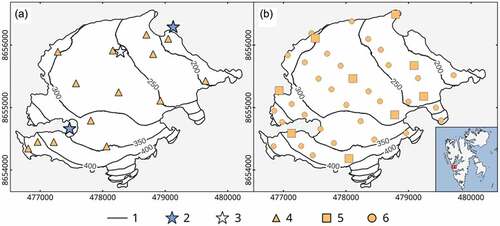
The last stake reading in the preceding year, 2020, was taken on 10 September, and this date is assumed to be the start of the mass balance year 2020–2021. From that date and until the onset of the ice melt in the middle of July 2021, observations were not carried out, and no exact chronology of the snowmelt is available. During the summer of 2021, stake readings were performed from 15 July until 11 September every three to seven days. To translate the stake readings into water equivalent units, the ice density was assumed to be equal to 880 kg m⁻³.

Model description

The heat-balance equation

To study the heat fluxes controlling the surface melt of Aldegondabreen, the research team implemented a model based on the heat balance equation, using the approach of Wheler and Flowers (2011) with two major modifications: solar lighting is simulated using the ready-to-use System for Automated Geoscientific Analyses geographic information system (SAGA GIS) module, and the subsurface heat flux is computed from a subsurface model similar to that described by Klok and Oerlemans (2002) but with a greater number of subsurface layers. The meltwater is immediately taken away from the surface, and neither percolation nor refreezing is simulated.

The heat balance equation is formulated as follows:

(1) $\mathrm{A}=\mathrm{Q}\cdot \left(1-\mathit{\alpha }\right)+\mathrm{I}+\mathrm{P}+\mathrm{LE}+\mathrm{G}$(1)

where $\mathrm{A}$ is the energy available for melt, $\mathrm{Q}$ is the incoming shortwave radiation, $\mathit{\alpha }$ is the albedo of the underlying surface, $\mathrm{I}$ is the longwave radiation balance, $\mathrm{P}$ and $\mathrm{LE}$ are the vertical turbulent sensible and latent heat fluxes, and $\mathrm{G}$ is the subsurface heat flux. The time step of the simulation is 1 hour, so all of the fluxes in Equation (1)(1) $\mathrm{A}=\mathrm{Q}\cdot \left(1-\mathit{\alpha }\right)+\mathrm{I}+\mathrm{P}+\mathrm{LE}+\mathrm{G}$(1) are calculated as hourly averages. The calculation of each of the components is described below.

Shortwave balance

The $\mathrm{Q}\cdot \left(1-\mathit{\alpha }\right)$ component of Equation (1)(1) $\mathrm{A}=\mathrm{Q}\cdot \left(1-\mathit{\alpha }\right)+\mathrm{I}+\mathrm{P}+\mathrm{LE}+\mathrm{G}$(1) characterizes the shortwave balance of the glacier surface, including the flux of incoming shortwave radiation ($\mathrm{Q}$) and the reflective characteristic of the surface ($\mathit{\alpha }$). The model allows the distribution of the incoming $\mathrm{Q}$ values measured at a point over the entire surface of the glacier by taking into account the effects of shading and relief morphometry. The “potential incoming solar radiation” algorithm implemented in the System for Automated Geoscientific Analyses geographic information system (SAGA GIS) software was used, which made it possible to estimate the maximum available insolation at a certain time depending on both astronomical factors (the zenith and hour angle of the sun, the time of sunrise and sunset) and the terrain morphometry (slope, exposure, and shading by the sides of the valley; Boehner and Antonic 2009). The simulation was carried out with a discreteness of 15 minutes. Then, the model compared the directly measured value with the computed potential one at the corresponding pixel and computed the scaling factor to recalculate potential values into real ones.

The other input data for shortwave balance computation is the glacier surface albedo. Snow albedo varies in time, so the model should be provided with several albedo maps for the known moments of time. For the time steps in between, albedo is linearly interpolated for every pixel, which preserves its “class” (snow/ice) within the initial and end dates. For the pixels where snow melts out and bare ice is exposed in the next image, the albedo of snow depends on the date of the last snowfall. The equation for diminishing the snow albedo in time follows Rohrer and Braun (1994):

(2) $\mathit{\alpha }=\mathit{\hspace{0.17em}}{\mathit{\alpha }}_0+k^{(-\mathit{n}\cdot \mathit{r})}\mathit{\hspace{0.17em}}$(2)

where ${\mathit{\alpha }}_0$ is the minimum possible snow albedo value of 0.40, $\mathrm{k}$ = 0.44, $\mathrm{n}$ is the number of days since the last snowfall, and $\mathrm{r}$ is the recession constant, which was calibrated within a range of 0.05 to 0.15.

Longwave balance

The longwave balance (I) or the effective radiation of the Earth’s surface, which is the difference between the ascending and descending longwave radiation, was calculated according to the technique described in König-Langlo and Augstein (1994). According to this approach, the long-wavelength balance of the underlying surface is:

(3) $\mathrm{I}={\epsilon \sigma \mathrm{T}}_s^4\mathit{\hspace{0.17em}}-\mathit{\hspace{0.17em}}{\mathit{\epsilon }}_a\mathit{\sigma }{\mathrm{T}}^4\mathit{\hspace{0.17em}}$(3)

The first term in Equation (3)(3) $\mathrm{I}={\epsilon \sigma \mathrm{T}}_s^4\mathit{\hspace{0.17em}}-\mathit{\hspace{0.17em}}{\mathit{\epsilon }}_a\mathit{\sigma }{\mathrm{T}}^4\mathit{\hspace{0.17em}}$(3) is the upward longwave radiation flux, where ${\mathrm{T}}_s$ is the absolute surface temperature, $\mathit{\sigma }$ is the Stefan-Boltzmann constant of 5.669⋅10⁻⁸ W/(m²⋅K⁴), and $\mathit{\epsilon }$ is the emissivity of the surface. Different values of emissivity $\mathit{\epsilon }$ have been proposed in glacier studies, ranging between 0.98 and 1.0, so we chose the best-fit value during model calibration.

The second term of Equation (3)(3) $\mathrm{I}={\epsilon \sigma \mathrm{T}}_s^4\mathit{\hspace{0.17em}}-\mathit{\hspace{0.17em}}{\mathit{\epsilon }}_a\mathit{\sigma }{\mathrm{T}}^4\mathit{\hspace{0.17em}}$(3) is the downward radiation of the atmosphere, where ${\mathit{\epsilon }}_a$ is the emissivity of the atmosphere, which is a function of the amount of cloudiness, air temperature, and water vapor pressure at a height of 2 m.

Turbulent fluxes

The calculation of turbulent fluxes of sensible (P) and latent (LE) heat was carried out by a method based on the semi-empirical Monin-Obukhov theory of turbulence (Munro 1990). This method has been widely used to model the melt of mountain glaciers, and the results have been presented in a number of papers (Hock 2005; Wheler and Flowers 2011; Prokhorova et al. 2021). To estimate the values of P and LE fluxes, bulk aerodynamic formulas are used, which include the wind speed, temperature, and relative air humidity at two heights, 0 and 2 m above the surface. The equations are as follows:

(4) $\mathit{P}=C_H{c}_p{\rho }_a{u}_z\cdot \left(T_z-T_s\right)$(4)

(5) $\mathit{LE}=C_E{L}_v{\rho }_a{u}_z\cdot \left(\frac{0.622}{P}\right)\left(e_z-e_s\right)$(5)

where $C_H$ and $C_E$ are the turbulent heat transfer coefficients (Hock and Holmgren 1996), ρa is the air density calculated from its temperature and pressure, $c_p$ = 1,010 J/(kg⋅K) is the specific heat of air, and $L_v$ = 2.514⋅10⁶ J/kg is the latent heat of vaporization (or sublimation, depending on the surface temperature). Wind speed $u_z$, air temperature $T_z$, and pressure $\mathit{P}$ were measured at a height of $\mathit{z}$ = 2 m. The partial pressure of water vapor at height z was computed from the measured relative humidity of the air. The surface temperature $T_s$ was computed from the multilayer subsurface model described below. Computation of the turbulent transfer coefficients requires the values of the surface roughness $z_0$. These are not time dependent in the model, but the values for the ice and snow may be different. $z_{0\mathit{m}}$ for momentum were obtained from model calibration, and the values for heat and water vapor were assumed to be 1/100 of $z_{0\mathit{m}}$.

Subsurface flux

The subsurface, or conductive, energy flux G was computed from the vertical temperature gradient ∇T in an upper layer of the multilayer subsurface model, which extends the simple two-layer model by Klok and Oerlemans (2002):

(6) $\mathit{G}=\mathit{k}\mathrm{\nabla }{T}_{\mathit{surf}}\mathit{c\rho }$(6)

where $\mathit{c}$ is the specific heat capacity, $\mathit{\rho }$ is the density, and k is the effective conductivity, depending on the bulk material density in the upper layer (Sturm et al. 1997):

(7) $\mathit{k}=0.138-1.01\cdot {10}^{-3}\mathit{\rho }+3.233\cdot {10}^{-6}{\rho }^2$(7)

The change in the temperature of the upper layer within every model time step is computed as follows:

(8) $\frac{\mathrm{\partial }{\mathit{T}}_{\mathit{surf}}}{\mathrm{\partial t}}=\frac{\mathit{k}\mathrm{\nabla }\mathit{T}}{{\mathit{d}}_{\mathit{surf}}}+\frac{B}{\mathit{c\rho }{\mathit{d}}_{\mathit{surf}}}$(8)

where $d_{\mathit{surf}}$ is the thickness of the upper layer, and $\mathit{B}$ is the atmospheric heat flux, which is a sum of short- and longwave surface energy balances and turbulent fluxes. $\mathit{B}$ is applied only for the topmost layer of the multilayer subsurface model; for deeper layers, a temperature change is controlled only by the difference of up- and downwelling conductive heat fluxes.

Model initialization

Digital elevation model

As a digital elevation model (DEM) of the glacier surface, we used a fragment of the ArcticDEM elevation model for the year 2013. The DEM was used for (1) distributing the measured weather parameters across the glacier surface based on the measured vertical gradients and (2) computing potential incoming solar radiation flux at the surface.

Weather data

The meteorological and actinometric data used to force the model were obtained directly from the Aldegondabreen glacier. Two Hobo automatic weather stations (AWSs) were installed permanently in the lower (ca. 180 m.a.s.l.) and higher (ca. 340 m.a.s.l.) parts of the glacier on the moraine (Figure 1). These AWSs measured the weather conditions air temperature, relative humidity, atmospheric pressure, wind speed and direction, and incoming solar radiation in the range of 300 to 1,000 µm. AWSs have been operating from 2015 to the present.

An additional seasonal heat balance mast was installed on a flat, nonshaded, homogeneous site (ca. 260 m.a.s.l.) on the Aldegondabreen surface during the summer melt period of 2021. The mast measured fluxes of incoming and reflected shortwave radiation in the wider range of 300 to 3,000 µm. These data were used to compute the adjustment factor for solar radiation measured at the Hobo AWSs, which related to the truncated wavelength range.

For each time step, air temperature, relative humidity, and atmospheric pressure were inter- and extrapolated over the whole glacier surface using the corresponding measured vertical gradient values. The wind speed was used as a nondistributed parameter. The measured value was attributed to the whole glacier surface at every time span. Another lumped input (cloudiness) was deduced from the difference between the total potential incoming solar radiation flux and the observed one. The cloudiness score in tenths of the sky, with three grades of 0.2, 0.5, and 0.8, was determined by the ratio between the fluxes. This approach was used because the cloud cover in the archipelago is very heterogeneous, and the observations at the weather station in Barentsburg are poorly representative of the glacier.

Snow cover data

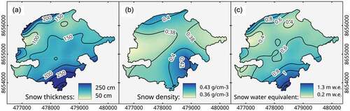
To simulate the surface ablation from the very beginning of the melt season, the grid of a snow water equivalent (SWE) was needed to initialize the model. To obtain the needed data, a detailed snow survey was carried out on 22 to 23 April 2021. The survey comprised nine pits for both snow density and thickness measurements and thirty-one additional points of snow thickness probing. The measurements were positioned in a quasi-regular grid (Figure 1b). To obtain an SWE grid used to initialize the model, the research team first interpolated snow thickness and bulk (depth-averaged) snow densities using the thin plate spline algorithm and then multiplied them (Figure 2). The area-averaged SWE for spring 2021 equaled 0.63 m water equivalent (w.e.). The mean snow density, used to compute the conductive heat flux, was 387 kg m⁻³.

Figure 2. Snow cover of Aldegondabreen in spring 2021: (a) snow thickness, (b) depth-averaged snow density, and (c) snow water equivalent.

Subsurface temperature profile

An initial subsurface temperature profile needed to initialize the multilayer model was computed from the measurements at the thermistor string on the date of model start, 10 May (Figure 3). The GeoPrecision thermistor string, with an accuracy of 0.1°C, distance between sensors of 0.5 m, and total length of 5.0 m, was used. It was installed near the heat balance mast in April before the onset of melt. At the date of model start, the topmost 0.5 m of the string was inside the snow cover. The time step of the measurements was set to 1 hour to match all of the other observations at the AWSs and heat balance mast.

Figure 3. The subsurface temperature profile from the thermistor string (zero depth is the snow/ice boundary) for 10 May 2021 (12:00) used for model initialization.

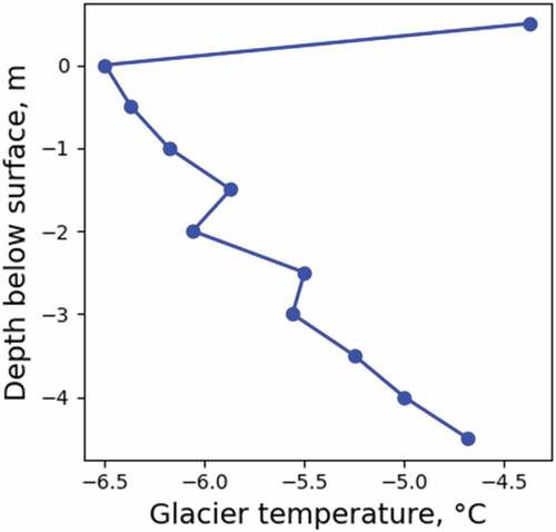
We did not use the measurements of the subsurface temperature to validate the model output at every time step. The challenge is that the glacier surface is lowering during the melt season relative to the string, and therefore the distance between the surface and the nearest sensors is not known. This makes it impossible to attribute measured temperatures to certain depths in the model.

Surface albedo

As a surface albedo input, we used nine cloudless space images taken by the Sentinel-2 satellite (Table 1). The narrow-to-broadband albedo regression-based conversion described in Naegeli et al. (2017) was applied to all scenes. The regression involved five spectral bands of 10- and 20-m spatial resolution:

(9) $\begin{array}{rl}\mathit{\alpha }& =0.356b_2+0.130b_4+0.373b_8+0.085b_{11}\\ & +0.072b_{12}-0.0018\end{array}$(9)

Table 1. Satellite imagery used for model initialization and calibration/validation.

Date	Satellite	Albedo input	Snowline delineation
23 April 2021	Sentinel-2	+	−
15 May 2021	Sentinel-2	+	−
23 May 2021	Sentinel-2	+	−
6 June 2021	Sentinel-2	+	+
11 June 2021	Landsat-8	−	+
27 June 2021	Landsat-8	−	+
6 July 2021	Landsat-8	−	+
23 July 2021	Sentinel-2	+	+
9 August 2021	Sentinel-2	+	+
28 August 2021	Sentinel-2	+	+
3 September 2021	Sentinel-2	+	−
7 September 2021	Sentinel-2	+	−

where α is the broadband albedo and b_i is the surface reflectance in the indicated Sentinel-2 spectral bands. This equation outputs the shortwave broadband albedo considering the wavelength from 380 to 2,500 nm; the sensor used to measure the solar irradiance has a range of 300 to 3,000 nm. Due to the very small values of solar irradiance at wavelengths larger than 2,400 nm and a low atmospheric transmittance at wavelengths shorter than 380 nm (Lucht et al. 2000), it is possible to use the equation without any additional coefficients and conversions.

Model calibration/validation

The model uncertainty was evaluated versus three parameters: (1) changes in the snow cover area fraction (SCAF) in time, (2) cumulative point ice melt at the fourteen stakes, and (3) point ice melt rates within all of the measured in situ time spans.

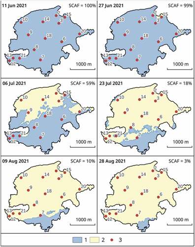
It is hard to quantitatively define the truthfulness of the modeled spatial distribution of snow except by means of the SCAF parameter. To estimate the real SCAF, the research team delineated the snow line on several satellite images (Table 1). The result of delineation and the SCAF values used for model calibration are shown in Figure 4.

Figure 4. Temporal changes in a snow cover area fraction (SCAF) used for model calibration/validation: (1) snow cover, (2) bare ice, and (3) ablation stakes and their numbers.

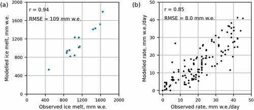
The second parameter, cumulative melt measured at the stakes, was treated by minimizing the root mean square error value and maximizing the Pearson correlation coefficient. As a measured cumulative melt, the difference between stake readings on 15 July and 11 September 2021 was used. We intentionally did not use the values of the preceding time span (since September 2020), because some extra ice melt might have occurred during the previous autumn, which did not fall within the modeling time period.

The third parameter was used to check whether the model made systematic errors during different parts of the ablation season. Theoretically, the cumulative melt may be predicted even with serious errors for shorter time spans, if they compensate for each other. Obviously, that case would not be useful for studying the intra-annual changes in the heat fluxes. Thus, we normalized all of the stake measurements by dividing them by the number of days between stake readings, obtaining the ice melt rates in centimeters per day. The calibration goal was to minimize the Pearson r value.

Model parameters used for model calibration are listed in Table 2. The calibration was performed by iterating over the values of the model parameters within a reasonable range. A best guess for parameters was defined through optimization of the three aforementioned criteria.

Table 2. Parameters used for the model calibration.

Parameter	Range	Best guess
Thermal emissivity of the ice/snow	0.98–1.00	0.98
Zm for the ice	0.2–2.0 mm	1.0 mm
Zm for the snow	0.2–2.0 mm	0.5 mm
Exponent in the equation for diminishing the snow albedo	0.05–0.15	0.12
Maximum albedo of the bare ice	0.45–0.55	0.45

Results and discussion

Model uncertainty

The values of all three quality metrics (Figure 5) were considered high in light of the model constraints and the uncertainties of the measurements used for validation.

Figure 5. Results of the model evaluation of (a) ice melt and (b) rate. RMSE = Root mean square error.

A major model constraint is that it does not account for any form of precipitation. Both liquid and solid precipitation may affect the surface albedo, decreasing or enhancing it, respectively. However, it is a challenging task to inter- or extrapolate precipitation over the glacier surface and even more challenging to verify the aforementioned effects due to the insufficient frequency of the available satellite imagery.

Stake measurements suffer from several major error sources. First of all, the translation from linear units to the water equivalent is based on the ice density assumption. This study used a value of 880 kg m⁻³, as suggested by colleagues carrying out long-term monitoring on the Austre Grønfjordbreen glacier to the south of Aldegondabreen (Chernov et al. 2019). However, other values, both higher and lower, have been presented in other publications. Huss (2013) proposed a very broad uncertainty limit for the ice density of 850 ±60 kg m⁻³, but this considers the presence of firn layers with a lower density. Based on our observations, Aldegondabreen does not currently possess the extensive firn zone as a result of the constant negative mass balance within the past decades; therefore, we considered it reasonable to narrow the uncertainty to ±30 kg w.e. This corresponds to a relative error of about 3.5 percent for every stake measurement. Moreover, the discussed model does not use ice density for recomputation, because all of the heat-specific parameters are nominated per kilogram, which is directly translated into w.e. units (1 kg of meltwater per 1 m² equals 1 mm w.e.).

Another uncertainty source is the stake measurement itself, resulting from stake inclination, sinking or floating, and other “technical” difficulties. Chernov et al. (2019) estimated this uncertainty to be no more than 2 cm (or ±17 mm w.e.). If one propagates this value with the previously discussed value of ice density uncertainty, one can obtain a combined uncertainty of ca. 40 mm w.e. for every 1,000 mm w.e. of ice ablation.

Moreover, every point measurement has limited representativeness: ice ablation varies in space not only with altitude but also in the lateral direction. In addition, the discussed model suffers from spatial averaging, because the input data have certain limitations with regard to spatial resolution. The crucial input, albedo maps derived from Sentinel-2 imagery, have a resolution of 20 m, which impedes a precise point-to-point comparison. Thus, we consider that model uncertainty is in accordance, overall, with the measured in situ ice melt values.

Surface energy budget

The heat balance observations lasted for 125 days. They were started on 10 May before the onset of snowmelt and lasted until 11 September, when the melt flux became near zero. The first melt, according to the model, occurred on Aldegondabreen in the last week of May (Figure 6).

Figure 6. Modeled intra-annual changes in the daily averaged heat fluxes on Aldegondabreen during the ablation season of 2021. SWD = shortwave downward flux; RS = shortwave radiation balance; RL = longwave radiation balance.

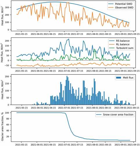
The maximum potential incoming solar radiation should occur on 21 June, which is the summer solstice. However, due to weather events, there was no distinct peak in the observed downwelling flux. All observed values were relatively high in the first half of the record, from 5 May to 7 July. Intense melt was not observed until 15 June, and the major part of the energy influx was spent on warming the snow to its melting point.

The peak of the melt flux was observed during the first week of July, when the snow line began to retreat up the glacier, decreasing its surface-averaged albedo. The latter snowline retreat occurred under the significantly reduced solar radiation flux, thus decreasing the amount of melt. In August to September, the incoming solar radiation gradually decreased, and several cases were observed when the turbulent fluxes supplied the heat amount comparable to that of the shortwave balance or even higher (Figure 7). The sensible heat flux has been positive since the start of weather observations. The latent heat flux became steadily positive on 26 June and remained until the beginning of September. This means that condensation from air moisture occurred over the glacier surface, in contrast with a study by Zou et al. (2021), where LE was identified to be the heat sink during the whole melt season.

Figure 7. The relative contribution of the different heat balance components to the heat inputs and heat sinks.

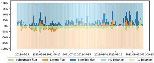
The ratio of the shortwave balance (84 percent) and sensible flux (13 percent) in the total heat influx (Table 3) was close to that computed for Austre Lovénbreen in 2014 (Zou et al. 2021), equaling 87 and 13 percent, respectively. However, it is hard to compare these estimates directly, because the latter were computed at a certain point on the glacier, whereas the present estimates were glacier-averaged.

Table 3. Mean heat fluxes over the Aldegondabreen surface during the melt season 2021 and their contribution to the heat influx.

Flux	Value (W/m^2)	Contribution (%)
Shortwave balance	83.2	84
Sensible heat flux	12.6	13
Latent heat flux	3.2	3
Subsurface heat flux	−3.9	—
Longwave balance	−45.7	—

The observed ratio between input energy sources has an important implication for formulating the condition when winter snow accumulation fully compensates for the summer melt. A previous study concerning Aldegondabreen’s sensitivity to the changes in temperature and precipitation considered that the amount of winter snow compensated for the ice melt in a 1:1 ratio (Osokin et al. 2010). This was deduced from the fact that the specific heat of fusion for ice and snow is equal, but this would be true only in the case when a primary driver for the melt is the air temperature. However, when the primary heat influx is solar radiation, snow ablation will be less intense than ice ablation, depending on their $\left(1-\mathit{\alpha }\right)$ ratio, or roughly three times. Therefore, 1 m w.e. of snow cover may compensate for 3 m w.e. of ice, which is much higher than the previous estimates and makes Aldegondabreen much more sensitive to changes in solid precipitation.

Events of increased turbulent fluxes

During the observations, several cases were identified when the role of turbulent heat fluxes significantly increased. Since the onset of a stable surface melt on 15 June, six events may be distinguished. A formal threshold for the event detection may be proposed: the sum of sensible and latent fluxes should be more than their mean seasonal value (16 W/m²) plus its standard deviation (20 W/m²), or 36 W/m². These events were episodic and ranged in duration from one day to one week, contributing to up to 60 percent of the total daily energy influx in August and September, when the solar radiation was low (Figure 7). If one sums all of the positive energy fluxes within the observation time span, the total heat influx is equal to 1,086.8 MJ, of which the turbulent fluxes within the six events contributed up to 105.3 MJ, or 10 percent.

The weather conditions, which were similar for all events, were strong winds and increased wind gust speed (Figure 8) in one prevalent direction. The research team compared the synoptic situation on the days of the events, and in all observed cases it was represented either by the passage of a cyclone or by a trough of a cyclone to the west from the Atlantic shore of Spitsbergen (Table 4). This caused strong southerly and southeast winds and a consecutive increase in a turbulent flow. We did not split event number 1 into two parts despite the short decrease in the turbulent fluxes below the threshold value in its middle, because the whole event could be attributed to the one synoptic situation.

Figure 8. The events of significantly increased turbulent heat fluxes over the Aldegondabreen during the melt season of 2021.

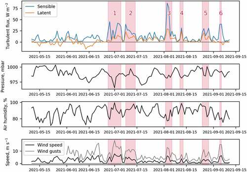
Table 4. The synoptic situation during the events of significantly increased turbulent fluxes over the Aldegondabreen during the melt season 2021.

Event number	Dates	Duration (days)	Synoptic situation
1	27 June–5 July	9	Deep cyclone, prevailing south and southeast wind direction, increase in gust wind speed (gust 18 m/s)
2	8 July–14 July	7	Cyclone trough, southeast wind direction, increase in gust wind speed (gust 11 m/s)
3	2 August–6 August	5	Deep cyclone, prevailing south and southeast wind direction, increase in gust wind speed (gust 12 m/s)
4	12 August	1	Center of cyclone, southeast wind direction, increase in gust wind speed (gust 7 m/s)
5	25 August–29 August	5	Col or saddle point, southeast wind direction, increase in gust wind speed (gust 11 m/s)
6	5 September–6 September	2	Cyclone trough, south and southeast wind direction (gust 15 m/s)

Shestakova et al. (2022) described the foehn winds observed over the Svalbard archipelago in May 2017 during easterly flow, which resulted in an increase in temperature and sensible heat flux, which suggests a potentially large effect on the snow cover and the glacier energy and mass balance. Several factors make it impossible to identify the observed events as foehns: (1) the wind direction is in accordance with the general atmospheric circulation, and no topographic modulation is seen; (2) there was no drop in air humidity, which occurs due to the adiabatic expansion of air during foehns, and the latent flux increased as well; (3) the events are not characterized by air warming—the primary factor that increased turbulent fluxes is the wind speed itself, not the air temperature. Thus, it can be concluded that the primary driver of the significantly increased turbulent fluxes over Aldegondabreen was the cyclonic activity.

The future projections of cyclonic activity around the Svalbard archipelago were recently assessed by Akperov et al. (2019). The analysis based on the regional climate model Arctic CORDEX (RCP 8.5) showed an increase in cyclones during the winter but produced an ambiguous result for the summer period, with different trend signs for different models. Thus, the future trends of cyclones around Svalbard remain debatable. However, studies regarding the recent changes in cyclonic activity showed that there was no significant increase in the number of cyclones in summer, but there was a transition in the origin of cyclones from zonal to meridional transport (Svyashchennikov, Prokhorova, and Ivanov 2020; Łupikasza et al. 2021). In winter, the number of cyclones at high latitudes in the North Atlantic sector increased over the period 1979 to 2016 according to reanalysis data (Wickström et al. 2019). The frequency of extreme cyclones passing in the subarctic part of the North Atlantic also increased (Koyama et al. 2017; Wickström et al. 2019). Rinke et al. (2017) showed that this trend was mainly due to increased cyclonic frequency in November to December and attributed it to the reduction in sea-ice conditions. This may potentially prolong the glacier surface melt in the autumn and decrease the accumulation of solid precipitation along the Atlantic coast of Spitsbergen.

Conclusions

The length of the observational series on Aldegondabreen during the melt season of 2021 was 125 days (10 May to 11 September). The modeling results confirm that the dominant contributor to the surface heat balance of the low-elevation Svalbard glacier was solar radiation: the mean shortwave budget was equal to 83.2 W/m² or 84 percent. The other two energy inputs were the sensible (12.6 W/m² or 13 percent) and latent (3.2 W/m² or 3 percent) heat fluxes. This means that these glaciers are highly sensitive to the winter accumulation of snow, which modulates the surface albedo during the summer peak of insolation.

The reported ratio is true for a timescale of the whole melt season, but within some days or hours, turbulent fluxes outweigh the shortwave balance. Six events of significantly increased turbulent fluxes were observed. During August and September, when solar radiation is low, these events supplied up to 60 percent of the daily heat influx. All events were characterized by cyclonic activity to the west from Svalbard, resulting in strong southern winds over the study area. The turbulent fluxes during these six events contributed to about 10 percent of the total heat input, and recent studies showed that the cyclonic activity near Svalbard tends to increase. This could lead to a longer melt season on the glaciers of the western Atlantic coast.

Author contributions

U.P. contributed to study conceptualization, methodology and validation; A.T. implemented the software; V.D. provided resources for model calibration and validation; U.P. and A.T. were responsible for writing the original draft of the article; V.D. and B.I. wrote, reviewed, and edited the article; and B.I. was responsible for project administration. All the authors read and agreed to the published version of the article.

Acknowledgments

The authors are grateful to the management and scientific staff of the Russian Arctic Expedition on Svalbard (Arctic and Antarctic Research Institute, Saint Petersburg, Russia) for providing logistics and the needed equipment for carrying out the field studies. The authors offer their special thanks to Kseniia Romashova for providing snow survey data.

Disclosure statement

No potential conflict of interest was reported by the author(s).

Additional information

Funding

This study was funded by Roshydromet, “Monitoring of State and Pollution of the Environment, Including the Cryosphere, in the Arctic Basin and in the Area of Scientific Station Ice Base Cape Baranov, Hydrometeorological Observatory of Tiksi and Russian Scientific Centre on Spitsbergen” within Project 5.1.4 of Plan NITR of Roshydromet 2020-24.

References

- Aas, K. S., T. Dunse, E. Collier, T. V. Schuler, T. K. Berntsen, J. Kohler, and B. Luks. 2016. The climatic mass balance of Svalbard glaciers: A 10-year simulation with acoupled atmosphere–glacier mass balance model. The Cryosphere 10 (3):1089–13. doi:10.5194/tc-10-1089-2016.
- Akperov, M., A. Rinke, I. I. Mokhov, V. A. Semenov, M. R. Parfenova, H. Matthes, M. Adakudlu, F. Boberg, J. H. Christensen, M. A. Dembitskaya, et al. 2019. Future projections of cyclone activity in the Arctic for the 21st century from regional climate models (Arctic-CORDEX). Global and Planetary Change 182:103005. doi:10.1016/j.gloplacha.2019.103005.
- Arnold, N. S., W. G. Rees, A. J. Hodson, and J. Kohler. 2006. Topographic controls on the surface energy balance of a high Arctic valley glacier. Journal of Geophysical Research 111 (F2). doi:10.1029/2005JF000426.
- Böhner, J., and O. Antonić. 2009. Land surface parameters specific to topo-climatology. Development of Soil Sciences 33:195–226.
- Borisik, A. L., A. L. Novikov, A. F. Glazovsky, I. I. Lavrentiev, and S. R. Verkulich. 2021. Structure and dynamics of Aldegondabreen, Spitsbergen, according to repeated GPR surveys in 1999, 2018 and 2019. Led i Sneg 61:26–37.
- Chernov, R. A., A. V. Kudikov, T. V. Vshivtseva, and N. I. Osokin. 2019. Estimation of the surface ablation and mass balance of Eustre Grønfjordbreen (Spitsbergen). Led i Sneg 59:59–66.
- Hock, R. 2005. Glacier melt: A review of processes and their modelling. Progress in Physical Geography: Earth and Environment 29 (3):362–91. doi:10.1191/0309133305pp453ra.
- Hock, R., and B. Holmgren. 1996. Some aspects of energy balance and ablation of Storglaciären, northern Sweden. Geografiska Annaler: Series A, Physical Geography 78 (2–3):121–31.
- Holmlund, E. 2021. Aldegondabreen glacier change since 1910 from structure-from-motion photogrammetry of archived terrestrial and aerial photographs: Utility of a historic archive to obtain century-scale Svalbard glacier mass losses. Journal of Glaciology 67 (261):107–16. doi:10.1017/jog.2020.89.
- Huss, M. 2013. Density assumptions for converting geodetic glacier volume change to mass change. The Cryosphere 7 (3):877–87. doi:10.5194/tc-7-877-2013.
- Klok, E., and J. Oerlemans. 2002. Model study of the spatial distribution of the energy and mass balance of Morteratschgletscher, Switzerland. Journal of Glaciology 48 (163):505–18. doi:10.3189/172756502781831133.
- König-Langlo, G., and E. Augsteine. 1994. Parameterization of the downward long-wave radiation at the Earth’s surface in polar regions. Meteorologische Zeitschrift 6 (6):343–47. doi:10.1127/metz/3/1994/343.
- Koyama, T., J. Stroeve, J. Cassano, and A. Crawford. 2017. Sea ice loss and Arctic cyclone activity from 1979 to 2014. Journal of Climate 30 (12):4735–54. doi:10.1175/JCLI-D-16-0542.1.
- Lucht, W., A. H. Hyman, A. H. Strahler, M. J. Barnsley, P. Hobson, and J. Muller. 2000. A comparison of satellite-derived spectral albedos to ground-based broadband albedo measurements modeled to satellite spatial scale for a semidesert landscape. Remote Sensing of Environment 74 (1):85–98. doi:10.1016/S0034-4257(00)00125-5.
- Łupikasza, E. B., D. Ignatiuk, M. Grabiec, K. Cielecka-Nowak, M. Laska, J. Jania, B. Luks, A. Uszczyk, and T. Budzik. 2019. The role of winter rain in the glacial system on Svalbard. Water 11 (2):334. doi:10.3390/w11020334.
- Łupikasza, E. B., T. Niedźwiedź, R. Przybylak, and Ø. Nordli. 2021. Importance of regional indices of atmospheric circulation for periods of warming and cooling in Svalbard during 1920–2018. International Journal of Climatology 41 (6):3481–502. doi:10.1002/joc.7031.
- Małecki, J. 2015. Glacio− meteorology of Ebbabreen, Dickson Land, central Svalbard, during 2008–2010 melt seasons. Polish Polar Research 36 (2):145–61. doi:10.1515/popore-2015-0010.
- Möller, M., R. Finkelnburg, M. Braun, R. Hock, U. Jonsell, V. A. Pohjola, D. Scherer, and C. Schneider. 2011. Climatic mass balance of the ice cap Vestfonna, Svalbard: A spatially distributed assessment using ERA-Interim and MODIS data. Journal of Geophysical Research 116 (F3):F03009. doi:10.1029/2010JF001905.
- Möller, M., and J. Kohler. 2018. Differing climatic mass balance evolution across Svalbard glacier regions over 1900–2010. Frontiers in Earth Science 6. doi:10.3389/feart.2018.00128.
- Munro, D. S. 1990. Comparisons of melt energy computations and ablatometer measurements on melting ice and snow. Arctic and Alpine Research 22 (2):153–62. doi:10.2307/1551300.
- Naegeli, K., A. Damm, M. Huss, H. Wulf, M. Schaepman, and M. Hoelzle. 2017. Cross-comparison of albedo products for glacier surfaces derived from airborne and satellite (Sentinel-2 and Landsat 8) optical data. Remote Sensing 9 (2):110. doi:10.3390/rs9020110.
- Noël, B., C. L. Jakobs, W. J. J. van Pelt, S. Lhermitte, B. Wouters, J. Kohler, J. O. Hagen, B. Luks, C. H. Reijmer, W. J. van de Berg, et al. 2020. Low elevation of Svalbard glaciers drives high mass loss variability. Nature Communications 11 (1):4597. doi:10.1038/s41467-020-18356-1.
- Nuth, C., J. Kohler, M. Konig, A. von Deschwanden, J. O. Hagen, A. Kaab, G. Moholdt, and R. Pettersson. 2013. Decadal changes from a multi-temporal glacier inventory of Svalbard. The Cryosphere 7 (5):1603–21. doi:10.5194/tc-7-1603-2013.
- Osokin, N. I., A. V. Sosnovsky, P. R. Nakalov, and R. A. Chernov. 2010. Assessment of ablation on the glaciers of the Svalbard archipelago at the beginning of the 21st century. Led i Sneg 3:13–18.
- Østby, T. I., T. V. Schuler, J. O. Hagen, R. Hock, and L. H. Reijmer. 2013. Parameter uncertainty, refreezing and surface energy balance modelling at Austfonna ice cap, Svalbard, 2004-08. Annals of Glaciology 54 (63):229–40. doi:10.3189/2013AoG63A280.
- Porter, C., P. Morin, I. Howat, M.-Y. Noh, B. Bates, K. Peterman, S. Keesey, et al. 2018. ArcticDem, Version 3. https://doi.org/10.7910/DVN/OHHUKH.HarvardDataverse,V1.
- Prokhorova, U. V., A. V. Terekhov, B. V. Ivanov, and S. R. Verkulich. 2021. Calculation of the heat balance components of the Aldegonda glacier (Western Spitsbergen) during the ablation period according to the observations of 2019. Kriosfera Zemli 25:50–60.
- Rinke, A., M. Maturilli, R. M. Graham, H. Matthes, D. Handorf, L. Cohen, S. R. Hudson, and J. C. Moore. 2017. Extreme cyclone events in the Arctic: Wintertime variability and trends. Environmental Research Letters 12 (9):Article 094006. doi:10.1088/1748-9326/aa7def.
- Rohrer, M. B., and L. N. Braun. 1994. Long-term records of snow cover water equivalent in the Swiss Alps: 2. Simulation. Hydrology Research 25 (1–2):65–78. doi:10.2166/nh.1994.0020.
- Schuler, T. V., J. Kohler, N. Elagina, J. O. M. Hagen, A. J. Hodson, J. A. Jania, A. M. Kääb, B. Luks, J. Małecki, G. Moholdt, et al. 2020. Reconciling Svalbard glacier mass balance. Frontiers in Earth Science 8:156. doi:10.3389/feart.2020.00156.
- Shestakova, A. A., D. G. Chechin, C. Lüpkes, J. Hartmann, and M. Maturilli. 2022. The foehn effect during easterly flow over Svalbard. Atmospheric Chemistry and Physics 22 (2):1529–48. doi:10.5194/acp-22-1529-2022.
- Strzelecki, M. C., A. J. Long, J. M. Lloyd, J. Małecki, P. Zagórski, Ł. Pawłowski, and M. W. Jaskólski. 2018. The role of rapid glacier retreat and landscape transformation in controlling the post-Little Ice Age evolution of paraglacial coasts in central Spitsbergen (Billefjorden, Svalbard). Land Degradation & Development 29 (6):1962–78. doi:10.1002/ldr.2923.
- Sturm, M., J. Holmgren, M. König, and K. Morris. 1997. The thermal conductivity of seasonal snow. Journal of Glaciology 43 (143):26–41. doi:10.1017/S0022143000002781.
- Svyashchennikov, P. N., U. V. Prokhorova, and B. V. Ivanov. 2020. Comparison of atmospheric circulation in the area of Spitsbergen in 1920–1950 and in the modern warming period. Russian Meteorology and Hydrology 45 (1):22–28. doi:10.3103/S1068373920010033.
- Troitsky, L. S., E. M. Singer, V. S. Koryakin, V. A. Markin, and V. I. Mikhaliov. 1975. Glaciation of the Spitsbergen. Moscow, Russia: Nauka. 276.
- Van Pelt, W. J. J., V. Pohjola, R. Pettersson, S. Marchenko, J. Kohler, B. Luks, J. O. Hagen, T. V. Schuler, T. Dunse, B. Noël, et al. 2019. A long-term dataset of climatic mass balance, snow conditions, and runoff in Svalbard (1957–2018). The Cryosphere 13 (9):2259–80. doi:10.5194/tc-13-2259-2019.
- Van Pelt, W. J., V. A. Pohjola, and C. H. Reijmer. 2016. The changing impact of snow conditions and refreezing on the mass balance of an idealized Svalbard glacier. Frontiers in Earth Science 4. doi:10.3389/feart.2016.00102.
- Wheler, B. A., and G. E. Flowers. 2011. Glacier subsurface heat-flux characterizations for energy-balance modelling in the Donjek Range, southwest Yukon, Canada. Journal of Glaciology 57 (201):121–33. doi:10.3189/002214311795306709.
- Wickström, S., M. O. Jonassen, T. Vihma, and P. Uotila. 2019. Trends in cyclones in the high latitude North Atlantic during 1979–2016. Quarterly Journal of the Royal Meteorological Society 146 (727):762–69. doi:10.1002/qj.3707.
- Zou, X., M. Ding, W. Sun, D. Yang, W. Liu, B. Huai, S. Jin, and C. Xiao. 2021. The surface energy balance of Austre Lovénbreen, Svalbard, during the ablation period in 2014. Polar Research 40. doi:10.33265/polar.v40.5318.