Assessment of Arctic sea ice and surface climate conditions in nine CMIP6 climate models

ABSTRACT

The observed retreat and anticipated further decline in Arctic sea ice holds strong climate, environmental, and societal implications. In predicting climate evolution, ensembles of coupled climate models have demonstrated appreciable accuracy in simulating sea-ice area trends throughout the historical period, yet individual climate models still show significant differences in accurately representing the sea-ice thickness distribution. To better understand individual model performance in sea-ice simulation, nine climate models were evaluated in comparison with Arctic satellite and reanalysis-derived sea-ice thickness data, sea-ice area records, and atmospheric reanalysis data of surface wind and air temperature. This assessment found that the simulated spatial distribution of historical sea-ice thickness varies greatly between models and that several key limitations persist among models. Primarily, most models do not capture the thickest regimes of multiyear ice present in the Wandel and Lincoln seas; those that do often possess erroneous positive bias in other regions such as the Laptev Sea or along the Eurasian Arctic Shelf. This analysis provides enhanced understanding of individual model historical simulation performance, which is critical in informing the selection of coupled climate model projections for dependent future modeling efforts.

KEYWORDS:

• Climate model assessment
• sea ice
• Arctic

Introduction

Arctic sea ice has declined dramatically over the previous century, foremost demonstrated by a persistent negative trend in sea-ice area observed from 1979 to the present (Laxon et al. 2013; Doscher, Vihma, and Maksimovich 2014; Stroeve and Notz 2018). Thinning of sea-ice regimes has also been confirmed, as the prevalence of perennial multiyear ice has diminished, being replaced by seasonal first-year ice (Maslanik et al. 2007; Kwok 2018; Stroeve and Notz 2018). This first-year sea ice is (1) thinner than perennial sea ice (Tschudi, Stroeve, and Stewart 2016), (2) more dynamic (Kwok, Spreen, and Pang 2013; Olason and Notz 2014; DeRepentigny et al. 2020b), and (3) further responsive to atmospheric and oceanic forcing (Newton et al. 2017; Kwok 2018; Overland 2020). Sea ice plays a critical role in Arctic atmosphere and ocean processes; modifying the thermal energy budget through high surface albedo and suppressing air–sea heat, moisture, and momentum fluxes (Førland et al. 2004; Karlsson and Svensson 2013; Thomson and Rogers 2014; Haine et al. 2015; Goosse et al. 2018; Mioduszewski, Vavrus, and Wang 2018; Stroeve and Notz 2018; Casas-Prat and Wang 2020; Timmermans and Marshall 2020). Beyond geophysical effects, reduced Arctic sea-ice cover is anticipated to have considerable societal effects, with potential increases in Arctic maritime activity (Aksenov et al., 2017; J. Chen et al. 2020; Sibul and Jin 2021), growing regional development (Harsem et al. 2015), and greater risk of coastal hazards to impact Arctic communities (Barnhart, Overeem, and Anderson 2014; Mioduszewski, Vavrus, and Wang 2018; Williams and Erikson 2021). Because the reality of an “ice-free” summer (sea-ice area less than 1 × 10⁶ km²) is predicted to occur before 2050 (J. Chen et al. 2020; SIMIP Community 2020; Wei et al. 2020; Vavrus and Holland 2021), accurate forecasting of sea ice is crucial to facilitate understanding and preparedness for future impacts.

Climate models participating in the Coupled Model Intercomparison Project’s sixth phase (CMIP6) have shown marked improvement in simulating sea-ice cover in comparison to prior phases. The multimodel mean of sea-ice extent generally captures the seasonal amplitude between March peak sea-ice area and the September low. Yet, most models underestimate the observed downward trend of sea-ice extent, and there is a wide inter-model spread during the summer months when the greatest negative trend occurs (Shu et al. 2020; SIMIP Community 2020; Long et al. 2021; Shen et al. 2021). Even models shown to best follow the observed seasonal sea-ice area and volume still experience numerous challenges in simulating the spatial distribution of sea-ice thickness (Davy and Outten 2020; Watts et al. 2021).

This research seeks to assess CMIP6 climate models’ ability to simulate historic sea-ice thickness, area, and related surface climate variables to provide a comprehensive understanding of areas, variables, and seasons, which these models may excel at simulating or fail to simulate. Intensive effort has been directed toward analyzing CMIP6 models’ sea-ice cover simulation in the interest of improving climate projection (Shu et al. 2020; SIMIP Community 2020; Shen et al. 2021; Watts et al. 2021). This research has found that the newest generation of models generally represents the seasonal cycle of ice and multimodel ensemble captures the historical trend in pan-Arctic sea-ice loss. Yet there are substantial differences in the regional and seasonal biases between different models’ estimations of sea ice. In the Arctic, climate model forecasts are crucial to stakeholders impacted by changing sea-ice conditions and dependent Arctic research efforts such as wave climate simulations (Casas-Prat, Wang, and Swart 2018), Arctic maritime transportation studies (Melia, Haines, and Hawkins 2016; J. Chen et al. 2020), and even future wildlife habitat projections (Hamilton et al. 2014). For example, research attempting to simulate and assess the future Arctic Ocean wave climate could potentially utilize multiple climate model projections of variables as forcings, including surface winds, sea-ice concentration and thickness, and even air and ocean temperatures. This application and others cannot utilize robust ensemble climate projections as inputs and are themselves computationally expensive to produce. Given the aforementioned large differences in regional and seasonal bias between models and that many research efforts do not have the computational power to employ a large multimodel ensemble, it is crucial that research making use of climate model data consider model projection characteristics and select the appropriate model for the given application (Wyburn-Powell, Jahn, and England 2022). Thus, by enhancing understanding of model simulation of sea ice and related surface climate variables (wind speed and surface air temperature), this research is intended to provide a broad resource for future Arctic research reliant on the accuracy of climate model projections. It should be recognized, however, that accurate simulation of historic conditions does not guarantee future projection accuracy. The inverse, consistent bias in simulating historical conditions, does imply model shortcomings, and thus the process of model selection using historical performance criteria is necessary and has been shown to significantly influence the trajectory of future projections (Knutti et al. 2017; Docquier and Koenigk 2021).

To assess model simulation, historic Arctic sea ice and related surface climate variables were evaluated from the beginning of the satellite era to the end of the CMIP6 historical experiment (1979–2014). The sea ice variables assessed included sea-ice thickness (SIT) and sea-ice area (SIA), and the surface climate variables assessed included surface wind speed (SWS) and surface air temperature (SAT). SWS and SAT were selected for analysis because they are important sea ice drivers and have pan-Arctic availability and reasonable accuracy from atmospheric reanalysis products. These variables were compared monthly with remote sensing derived data, reanalysis sea ice products, and atmospheric reanalysis products. SIT simulation was evaluated in comparison to both the Pan-Arctic Ice Ocean Modeling and Assimilation System (PIOMAS) SIT reanalysis and merged CryoSat-2-SMOS SIT measurements for 2011 to 2014. The National Snow and Ice Data Center (NSIDC) Sea Ice Index (SII) was used to assess model simulation of average monthly SIA and trends. Finally, ERA5 atmospheric reanalysis was used in assessing model simulation of both SAT and SWS variables. Supplementing the pan-Arctic analysis, model simulation of SIT within the Canadian Archipelago and the nearby Baffin Bay was analyzed.

Data and methods

Model selection

Models selected for evaluation were identified from a previous assessment that identified models that forecast a realistic amount of sea-ice loss while concurrently simulating a plausible global mean temperature change (SIMIP Community 2020). From these previously identified models, only those that provided both SIT fields (for spatial analysis) and the necessary variables for SIA assessment were analyzed. The nominal horizontal resolution of the analyzed climate models differs substantially. Model resolution has been found to influence the accuracy of models, with higher resolution models tending to exhibit better simulation of oceanic heat transfer (Docquier et al. 2019). The CMIP6 historical experiment provides historical simulation data in varying temporal resolution; in this research, monthly averages of simulated variables were assessed. Multiple simulation realizations (ranging up to ten) are available for all but two of the models evaluated, as shown in Table 1. The use of multiple realizations ideally reduces the effects of internal variability, leaving only the mean state of the simulated variable. However, the number of ensemble members needed to accomplish this can be substantial and varies considerably depending on the internal variability within the variable of interest and the acceptable level of error in estimating said variable (Milinski, Maher, and Olonscheck 2020). This analysis is outside the scope of the study and thus robust conclusions pertaining to the models’ physics are indeterminate. However, previous analysis has shown that large climate model ensembles generally fall within the interannual variability present in pan-Arctic sea ice, yet different models may diverge significantly in simulating the regional and seasonal mean state of sea ice (Wyburn-Powell, Jahn, and England 2022), thus warranting the performed analysis.

Table 1. Climate models evaluated within the study, individual ocean grid resolution, affiliated institution, and the number of ensemble members available/used.

Climate model	Sea ice grid resolution	Institution ID	Ensemble members
ACCESS-CM2	360 × 300	CSIRO-ARCCSS	5
CESM2-WACCM	384 × 324	NCAR	3
CNRM-CM6-1-HR	1,442 × 1,050	CNRM-CERFACS	1
GFDL-ESM4	720 × 576	NOAA-GFDL	1
GISS-E2-1-G	90 × 144	NASA-GISS	10
MPI-ESM-1-2-HAM	256 × 220	MPI-M	3
MPI-ESM-1-2-HR	404 × 802	HAMMOZ-Consortium	10
MRI-ESM2-0	363 × 360	MRI	10
NorESM2-MM	360 × 384	NCC	3

Sea ice evaluation

SIT accuracy is assessed through comparison with the Alfred Wegner Institute’s combined CryoSat-SMOS (CS2SMOS) Merged Sea Ice Thickness data product (Ricker et al. 2017) and PIOMAS sea-ice reanalysis data set. The merged satellite data product utilizes both CryoSat-2- and SMOS-derived SIT measurements. The combined analysis SIT product is enhanced to measure a greater range of SIT regimes, most notably, thin ice from SMOS (Kwok and Cunningham 2015; X. Wang et al. 2016). The CS2SMOS SIT product provides monthly coverage from October through April. However, full monthly data for October and April are incomplete, with the data set beginning in late October and terminating in early April; this may potentially introduce both positive and negative biases for both monthly means. The overlap between complete CS2SMOS data and the CMIP6 historical experiment begins in 2011 and ends in 2014. Given the brevity in this period of assessment and the inclusion of 2012—an anomaly, with lowest summer sea-ice extent on record—an additional basis of assessment was needed to evaluate the mean distribution of sea ice. For this purpose, the PIOMAS SIT reanalysis was used for SIT comparison monthly from 1979 to 2014 (Zhang and Rothrock 2003; Schweiger et al. 2011). PIOMAS provides monthly full-year coverage and allows for the annual sea-ice minimum occurring in September to be analyzed. Though CS2SMOS and PIOMAS are viable and recognized sources of data for SIT analysis, there are still considerable sources of uncertainty in both data sets that require further explanation. These limitations and uncertainties are expanded upon in the Discussion and conclusion section.

The process of model SIT comparison is described as follows: (1) the average was taken across ensemble members; (2) monthly sea-ice grids were linearly interpolated onto either the CS2SMOS or PIOMAS grid; (3) months were averaged across the entire analysis period, establishing a monthly SIT mean; and (4) model and reference grids were subtracted to create error maps and derive statistical measures. Grid cells where both model and reference agree on open water conditions were excluded from the derivation of statistical measures to reduce the effect of large open water areas during summer months. Following pan-Arctic analysis, regional analysis for the Canadian Archipelago was performed, and summary statistics were derived for the area. Regional analysis limits assessment to the coordinates between latitudes 60° N to 80° N and longitudes 50° W to 130° W, which effectively encompasses the Canadian Archipelago and Baffin Bay.

Evaluation of climate model SIA is assessed with monthly SIA values reported from the NSIDC’s SII (Peng et al. 2013; Meier et al. 2017). Arctic SIA is derived by multiplying sea-ice concentration (SIC) by the respective area of the climate model grid cell and then taking the sum of all climate model grid cells within the Arctic. In the event that SIA was not provided as output variable for the model, SIA was derived using the model’s SIC grid and matching ocean area grid. For all climate models, the average of all realizations was taken to create the ensemble mean SIA time series. These values were then compared with the NSIDC’s SII value to determine bias. In calculating SIA, the SII monthly values omit the “pole hole” where satellite-imaged SIC was historically unavailable. To allow for comparison, we assume that the SIC within the pole hole is 100 percent and add the missing area onto the monthly SIA total. Though this induces some degree of uncertainty into our analysis, this is assumed to be acceptable because the greatest pole hole values present before 1987 occur above 84° N where the ice pack is assumed to be largely consolidated at the pole and by 2007 the pole hole area is nearly negligible at the scale of our analysis at 0.029 × 10⁶ km².

Surface climate evaluation

The European Center for Medium Range Forecasts’ ERA5 atmospheric reanalysis provides reference for SAT and SWS simulation analysis. Both SAT and SWS were analyzed in comparison to ERA5 historical atmospheric climate reanalysis data product. In a study of atmospheric reanalysis products within the Arctic, ERA5 or ERA-interim (predecessor to ERA5) simulated SAT and SWS were found to have high correlation and low error in comparison to the observed Arctic surface climate, thus qualifying the reanalysis for use in comparison (Lindsay et al. 2014; Graham et al. 2019; Demchev et al. 2020). However, it should be noted that ERA5 possesses a warm bias under extremely cold winter conditions (Graham et al. 2019; C. Wang et al. 2019; Davy and Outten 2020; Demchev et al. 2020).

Results

Sea-ice thickness

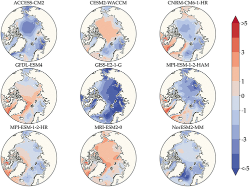
Comparison of model-simulated monthly SIT and averaged CS2SMOS observations for October and March over the four-year period 2011 to 2014 yields bias plots for October (Figure 1a) and March (Figure 1b). The summary statistics for both months are presented in Table 2 along with the overall statistics averaged over October through April. CS2SMOS data are unavailable for the annual sea-ice minimum month (September) and does not start until the latter half of the month of October. This potentially introduces a positive SIT bias into the month’s average used for comparison. Despite this, over half of the models exhibit a positive bias for October, ranging from 16 cm to over 1 m. For most models, this stems from an erroneous region of thick sea ice in East Siberian and Chukchi seas, most pronounced in the ACCESS-CM2, CESM2-WACCM, MPI-ESM-1-2-HAM, and NorESM2-MM models. This phenomenon has been previously observed as common to the majority of CMIP5 models analyzed (Stroeve et al. 2014), and it is notable that several models do not possess this feature. The three models with the highest mean positive bias for October are CESM2-WACCM, MPI-ESM-1-2-HAM, and NorESM2-MM, with mean bias values of 0.31, 0.44, and 1.06 m, respectively. CESM2-WACCM calculates a region of very thick ice (>2 m) at the outer edge of the sea-ice area for October in the Beaufort, Chukchi, an East Siberian seas (an anomalous feature not observed in other configurations of the model; DeRepentigny et al. 2020a), which results in the significant bias shown in these regions (see Figure 1a). It also simulates extremely thick ice (>6 m) at several locations within the Canadian Archipelago. MPI-ESM-1-2-HAM shows positive bias (>1 m) near the Laptev Sea, and the NorESM2-MM model has significant positive bias throughout the Arctic.

Figure 1. Sea-ice thickness bias (m) between model ensemble mean and CS2SMOS for (a) October and (b) March over the period 2011 to 2014.

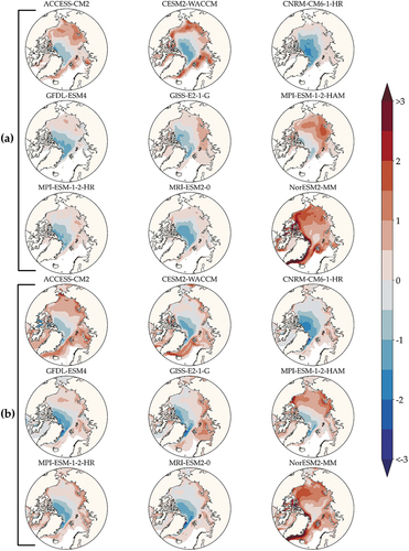
Table 2. Statistics of error between each model’s ensemble average and the reference CS2SMOS Analysis sea-ice thickness (SIT) for the individual months of October and March and an average of winter months (October through April) 2011 to 2014.

Model	ACCESS-CM2	CESM2-WACCM	CNRM-CM6-1-HR	GFDL-ESM4	GISS-E2-1-G	MPI-ESM-1-2-HAM	MPI-ESM-1-2-HR	MRI-ESM2-0	NORESM2-MM
October
RMSE	0.62	0.93	0.68	0.52	0.35	0.72	0.46	0.53	1.41
Mean bias	0.27	0.31	−0.34	−0.19	0.17	0.44	−0.09	−0.10	1.06
R	0.66	0.28	0.77	0.80	0.72	0.72	0.85	0.74	0.65
March
RMSE	0.68	0.77	0.57	0.57	0.90	0.66	0.55	0.58	1.16
Mean bias	0.34	0.22	−0.13	−0.09	0.66	0.29	0.08	0.08	0.80
R	0.79	0.67	0.83	0.81	0.51	0.83	0.82	0.79	0.76
Average (October–April)
RMSE	0.64	0.76	0.58	0.53	0.72	0.64	0.51	0.54	1.18
Mean bias	0.28	0.15	−0.20	−0.12	0.48	0.30	0.01	−0.03	0.81
R	0.77	0.61	0.80	0.80	0.54	0.81	0.82	0.78	0.74

Note. RMSE and mean bias in meters.

Previous climate model evaluations have shown that models typically underestimate especially thick sea-ice regimes. This holds true with the majority of models evaluated, which undercalculated the thick multiyear ice observed at the Wandel Sea, at the Lincoln Sea, and north of the Canadian Archipelago. CESM2-WACCM is able to simulate part of the sea-ice regime occurring along the northern coast of Greenland, yet it underestimates the continuation of the field toward the pole. MPI-ESM-1-2-HAM shows only slight underestimation (≈ −0.5 m) of the thickest sea-ice region during October, with bias growing into March. The only model to overrepresent ice in this region is the NorESM2-MM model, which shows significant positive bias throughout the Arctic. Recent research has shown the multiyear ice dominant in this region is more vulnerable to climate change than previously thought (Schweiger et al. 2021) and thus may be more responsive to climatic forcing (Overland 2020). In March, nearly all models show improved spatial correlation in comparison to October, because models typically struggle to capture the annual sea-ice minimum. Conversely, GISS-E2-1-G spatial correlation drops significantly from 0.72 to 0.51 from October to March; this is primarily attributed to significant overestimation of March sea-ice area far into southern Bering Sea and extending into the Pacific Ocean. All models show positive bias of varying magnitude and extent in the Laptev Sea and commonly extending into the East Siberian Sea. Models maintaining a correlation of r ≥ 0.8 overall are CNRM-CM6-1-HR, GFDL-ESM4, MPI-ESM-1-2-HAM, and MPI-ESM-1-2-HR. Of these, MPI-ESM-1-2-HR shows the lowest mean bias and the highest correlation coefficient.

Supplementing the comparison via CS2SMOS data, climate models were evaluated using the extended PIOMAS sea-ice reanalysis for 1979 to 2014. Differing in this step of assessment, September monthly averages are compared rather than October, which is used for CS2SMOS. Figure 2 shows almost all models possess increased agreement with PIOMAS; suspected drivers of this result include the lengthened time series and the fact that PIOMAS itself exhibits bias in several regions common to climate models, including the aforementioned positive bias in the East Siberian and Chukchi seas (Stroeve et al. 2014). Three models (ACCESS-CM2, CESM2-WACCM, MPI-ESM-1-2-HAM) simulate the thick sea ice north of Greenland, with negative bias less than >1 m in both March and September; all other models underestimate SIT in this region with the exception of NorESM2-MM, which has a pan-Arctic positive bias. Similar to the CS2SMOS comparison for October, CESM2-WACCM again has erroneously high SIT at the outer edge of the September sea-ice area, which drives the low correlation and high bias. Though MPI-ESM-1-2-HR performed best in comparison to CS2SMOS overall, MPI-ESM-1-2-HAM and GISS-E2-1-G performed markedly better in comparison to PIOMAS. The improved correlation coefficient of GISS-E2-1-G listed in Table 3 is notable, because this model exhibited the lowest correlation with CS2SMOS data. Further inspection of this result showed that this model exhibited negative bias in comparison to PIOMAS and large positive bias in comparison to the CS2SMOS data, suggesting that the model may not capture the thinning of sea-ice regimes in later years.

Figure 2. Sea-ice thickness bias (m) between model ensemble mean and PIOMAS for (a) October and (b) March over the period 2011 to 2014.

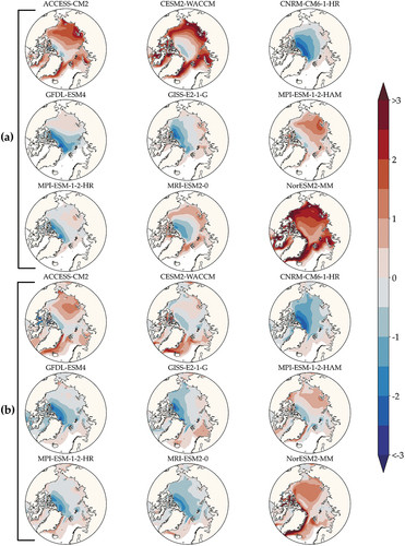
Table 3. Statistics of error between each model’s ensemble average and the reference PIOMAS reanalysis sea-ice thickness (SIT) for the individual months of September and March; and an average of all months 1979 through 2014.

Model	ACCESS-CM2	CESM2-WACCM	CNRM-CM6-1-HR	GFDL-ESM4	GISS-E2-1-G	MPI-ESM-1-2-HAM	MPI-ESM-1-2-HR	MRI-ESM2-0	NORESM2-MM
September
RMSE	1.04	1.57	1.02	0.90	0.68	0.66	0.64	0.70	2.01
Mean bias	0.68	1.05	−0.68	−0.59	−0.30	0.31	−0.30	0.07	1.65
R	0.72	0.45	0.82	0.75	0.87	0.84	0.87	0.76	0.67
March
RMSE	0.76	0.89	0.93	0.84	0.67	0.60	0.67	0.69	1.31
Mean bias	0.27	0.15	−0.60	−0.53	−0.23	0.01	−0.24	−0.42	0.77
R	0.83	0.73	0.87	0.86	0.89	0.87	0.88	0.93	0.78
Annual
RMSE	0.91	1.13	0.96	0.83	0.66	0.60	0.65	0.73	1.61
Mean bias	0.46	0.44	−0.63	−0.51	−0.23	0.12	−0.24	−0.21	1.11
R	0.78	0.62	0.85	0.84	0.89	0.87	0.87	0.82	0.73

Note. RMSE and mean bias in meters.

Canadian Archipelago sea-ice thickness

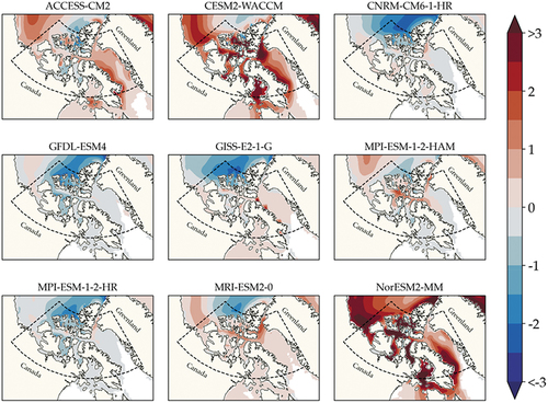
CMIP6 climate models have demonstrated positive biases for SIT within the Canadian Archipelago (Davy and Outten 2020). Investigating the performance of individual models in this region is relevant to understanding future development and maritime travel along Arctic sea routes such as the Northwest Passage. Our analysis in comparison to PIOMAS and the localized summary statistics in this area defined by latitudes 60° N to 80° N and longitudes 50° W to 130° W are provided in Table 4. CNRM-CM6-1-HR, GFDL-ESM4, GISS-E2-1-G, and MPI-ESM-1-2-HAM models had a correlation coefficient of r ≥ 0.8, with MPI-ESM-1-2-HAM having the lowest root mean square error (RMSE; as it did for the pan-Arctic assessment). The majority of models showed positive bias through most of the Canadian Archipelago, yet the three models with highest resolution (CNRM-CM6-1-HR, GFDL-ESM4, MPI-ESM-1-2-HR) trended toward negative bias for most of the region. These three models have similar SIT spatial distributions, as seen in Figure 3, and possess a strong negative bias in the Queen Elizabeth Islands in the northern part of the archipelago. GISS-E2-1-G trends toward overestimation of SIT throughout the region, with several isolated locations of intense SIT along the western part of Baffin Bay. As the model with coarsest spatial resolution, GISS-E2-1-G’s high correlation coefficient, comparable to that of the high-resolution models (CNRM-CM6-1-HR, MPI-ESM-1-2-HR) is unexpected, because model resolution would be expected to be a key factor in simulating sea-ice dynamics within the region (Docquier et al. 2019). Within the northern part of the Canadian Archipelago, CESM2-WACCM simulates localized extreme SIT values exceeding 10 m; this in part drives the poor spatial correlation and high error statistics for this model. By applying an SIT cutoff at 6 m (such as that applied by Watts et al. 2021), the model performance is improved markedly, because the correlation coefficient rises to 0.52 and the RMSE and mean bias fall to 1.3 m and 44 cm, respectively.

Table 4. Regional summary statistics of error for the Canadian Archipelago and Baffin Bay between each climate model and the reference PIOMAS sea-ice thickness (SIT) comparison for September 1979 to 2014.

Model	ACCESS-CM2	CESM2-WACCM	CNRM-CM6-1-HR	GFDL-ESM4	GISS-E2-1-G	MPI-ESM-1-2-HAM	MPI-ESM-1-2-HR	MRI-ESM2-0	NORESM2-MM
September
RMSE	0.93	1.70	0.90	0.98	0.72	0.62	0.74	0.69	1.81
Mean bias	−0.01	0.53	−0.62	−0.75	−0.29	−0.07	−0.34	−0.09	0.95
R	0.61	0.45	0.80	0.80	0.80	0.82	0.78	0.77	0.64

Note. RMSE and mean bias in meters.

Table 5. Model percentage error in comparison to the NSIDC observations in the September sea-ice area (SIA) linear trend (10⁶ km²/decade) for the period 1979 to 2014.

Model	ACCESS-CM2	CESM2-WACCM	CNRM-CM6-1-HR	GFDL-ESM4	GISS-E2-1-G	MPI-ESM-1-2-HAM	MPI-ESM-1-2-HR	MRI-ESM2-0	NORESM2-MM
March	15	3	7	1	24	4	2	2	4
September	14	0	15	11	62	7	−20	−19	42
Mean absolute percentage error	12	4	9	4	36	3	8	7	16
September SIA linear trend (10^6km^2/decade)	−0.79	−1.15	−0.44	−0.57	−0.57	−0.59	−0.61	−0.72	−0.37

Figure 3. Sea-ice thickness bias (m) between model ensemble mean and PIOMAS for September within the Canadian Archipelago 1979 to 2014. The delineation boundary is shown for selection of data used in deriving statistical measures.

Sea-ice area

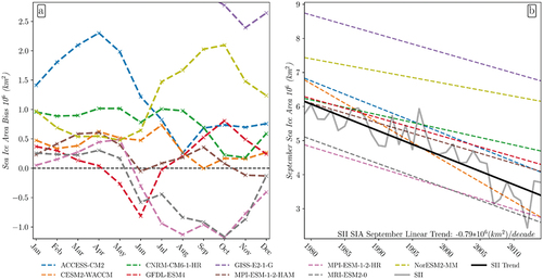
Sea ice coverage within the Arctic is a critical parameter in governing Arctic surface exchange of heat, mass, and momentum and thus has been the topic of several CMIP6 and CMIP5 studies (Shu et al. 2020; Shen et al. 2021). The current generation of CMIP6 climate models typically overrepresents SIA during both the seasonal maximum during March and the annual minimum during September (Shu et al. 2020). In this analysis, the majority of models overestimate SIA throughout the year with the exception of MPI-ESM-1-2-HR and MRI-ESM2-0, which both underestimate SIA in summer and fall months, as seen in Figure 4. GISS-E2-1-G shows considerably large positive bias through all months and largely exceeds the bounds of the bias plot shown on the left side of Figure 4. Examining the percentage error statistics shown in Table 5, the only models to achieve a mean absolute percentage error <5 percent over the annual cycle are CESM2-WACCM, GFDL-ESM4, and MPI-ESM-1-2-HAM. In comparison to winter months, models are observed to struggle in capturing the September SIA low, because all models’ percentage errors for this month rise significantly, with the exception of CESM2-WACCM at −0.04 percent. The observed and simulated linear trends in SIA loss for the month of September from 1979 to 2014 are shown in Figure 4b, and corresponding statistics are provided in Table 5. The best-fit line to observed SII September SIA has a slope of −0.79 × 10⁶ km²/decade, which is well captured by the model ACCESS-CM2 despite overrepresenting SIA for this month on average by approximately 0.6 × 10⁶ km². All models except for this one and CESM2-WACCM underestimate the rate of SIA decline for this period, which may contribute to the observed overestimation of SIA the majority of models show in this month.

Figure 4. Average monthly sea-ice area (SIA) bias for each climate model over the period 1979 to 2014. (b) Observed and simulated September SIA linear trend compared to the NSIDC record. GISS-E2-1-G is only shown in plot (a) for fall months, because error for this model exceeds +2.6 × 10⁶ km² for all other months and exceeds plot bounds.

Surface air temperature

The summary statistics derived from SAT analysis are presented in Table 6. Correlation coefficients are omitted from the statistical measure, because all models maintain annual correlation ≥0.97 when compared with ERA5 data. Examining mean error, all models except for MRI-ESM2-0 have negative annual bias. As previously mentioned, this is most likely driven by a previously acknowledged positive bias in ERA5 Arctic temperatures during the coldest winter months and further evidenced by the large negative mean bias values for the month of March shown in Table 6. Considering the potential effect this bias may have during colder months, assessment should prioritize September SAT performance where the ERA5 negative bias is not present and climate model mean bias values are more evenly distributed.

Table 6. Summary statistics for each climate model’s surface air temperature (°C) compared with ERA5 monthly surface air temperature within the region from 1979 to 2014.

Model	ACCESS-CM2	CESM2-WACCM	CNRM-CM6-1-HR	GFDL-ESM4	GISS-E2-1-G	MPI-ESM-1-2-HAM	MPI-ESM-1-2-HR	MRI-ESM2-0	NorESM2-MM
September
RMSE	2.5	1.5	1.7	1.2	4.1	2.4	1.0	1.6	1.6
Mean bias	−2.2	0.6	−1.2	0.7	−3.9	−2.0	−0.1	1.4	−1.2
March
RMSE	7.2	3.0	6.6	6.1	8.7	5.8	2.4	1.6	5.8
Mean bias	−6.8	−2.0	−5.9	−5.2	−7.8	−5.0	−1.7	−0.4	−5.3
Annual
RMSE	5.1	2.2	4.7	3.9	5.8	3.8	1.9	1.9	4.4
Mean bias	−4.1	−0.8	−3.7	−2.4	−4.8	−2.9	−0.6	0.2	−3.5

Note. RMSE and mean bias in °C.

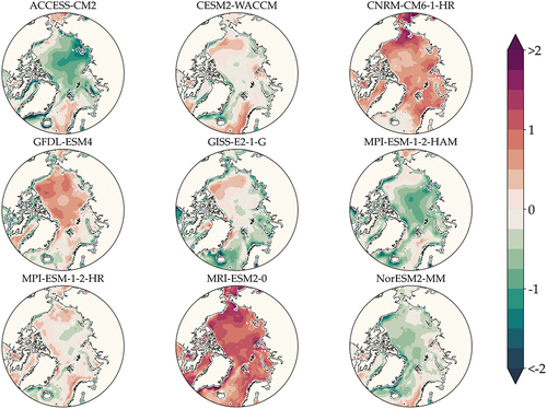
Temperature bias contour maps for the month of September can be seen in Figure 5. For September, the model with the lowest RMSE and mean bias is MPI-ESM-1-2-HR, at 1.0°C and −0.1°C, respectively. Examining the spatial bias of this model in Figure 5, it overestimates temperature for most of the seas surrounding Greenland and within the Canadian Archipelago (a feature observed in the majority of models) yet has minimal underestimation for the remainder of the Arctic. CNRM-CM6-1-HR, GFDL-ESM4, MPI-ESM-1-2-HAM, MPI-ESM-1-2-HR, and MRI-ESM2-0 all exhibit similar trends in high positive bias through the Canadian Archipelago, Baffin Bay, and Greenland Sea. GISS-E2-1 G, ACCESS-CM2, and MPI-ESM-1-2-HAM have consistent pan-Arctic negative bias, and ACCESS-CM2 and MPI-ESM-1-2-HAM also have large areas of negative bias reaching from the North Pole through the East Siberian Sea and into the Bearing Sea. MRI-ESM2-0 has the lowest mean annual bias of 0.2°C and is even with MPI-ESM-1-2-HR, with the lowest annual RMSE of 1.9°C. Investigating this result, the model shows minimal error during winter months (a result potentially driven by positive bias in ERA5 winter temperatures which are expanded upon the Discussion and Conclusion section) as shown for the month of March in Table 6. The previously discussed SAT positive bias within ERA5 under extreme cold weather may have had a significant influence in this result and thus demands future investigation and confirmation.

Figure 5. Surface air temperature bias for the month of September averaged over 1979 to 2014. Temperatures over land were excluded from analysis and masked over for mapping.

Surface wind speed

Analysis of SWS yields the summary statistics shown in Table 7. The spread in annual RMSE between models is less than 0.7 m/s and the range in annual bias values does not exceed 2 m/s. MPI-ESM-1-2-HR maintains the lowest RMSE out of all the models for September, March, and annually. Most models show improved correlation for March in comparison to September, with GFDL-ESM4 experiencing the largest improvement. Despite this, five out of the nine models show an increase in RMSE for this month. Because the ERA5 average of wind speeds for this month is approximately 0.5 m/s greater than September, this explains why certain models might show improved correlation for March while simultaneously exhibiting increased bias or RMSE.

Table 7. Summary statistics for each climate model’s surface wind speed simulation with ERA5 monthly surface wind speed within the region north of 60° N from 1979 to 2014.

Model	ACCESS-CM2	CESM2-WACCM	CNRM-CM6-1-HR	GFDL-ESM4	GISS-E2-1-G	MPI-ESM-1-2-HAM	MPI-ESM-1-2-HR	MRI-ESM2-0	NORESM2-MM
September
RMSE	0.79	0.33	0.68	0.63	0.49	0.70	0.29	1.02	0.51
Mean bias	−0.63	−0.08	0.62	0.35	−0.24	−0.60	−0.05	0.99	−0.41
R	0.90	0.93	0.93	0.75	0.84	0.91	0.93	0.95	0.95
March
RMSE	0.69	0.68	0.46	0.51	0.74	0.57	0.44	1.27	1.03
Mean bias	−0.40	−0.42	0.21	0.13	−0.37	−0.40	−0.19	1.22	−0.92
R	0.91	0.94	0.96	0.93	0.88	0.96	0.96	0.97	0.95
Annual
RMSE	0.75	0.63	0.56	0.54	0.62	0.69	0.41	1.07	0.94
Mean bias	−0.51	−0.39	0.37	0.13	−0.23	−0.54	−0.16	0.99	−0.73
R	0.90	0.93	0.94	0.90	0.88	0.95	0.95	0.96	0.89

Note. RMSE and mean bias in meters per second.

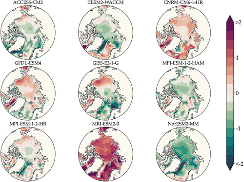
In Figure 6, the spatial bias contours can be used to elucidate the September statistics provided in Table 7. CNRM-CM6-1-HR and MRI-ESM2-0 immediately stand out as exhibiting pervasive positive bias not only for oceanic regions but also within coastal areas. A common feature in many of the models shown is a tendency for coastal areas to have considerable negative bias. This can be observed for the majority of models in the Beaufort Sea or along the southeast coast of Greenland. MPI-ESM-1-2-HR noticeably shows little bias exceeding 0.5 m/s.

Figure 6. Monthly surface wind speed bias averaged for September 1979 through 2014. Only surface winds corresponding to oceanic grid cells were considered for analysis.

Analyzing the March wind field bias shown in Figure 7, many models show areas of intense negative or positive bias in certain regions that were not observed in September. For example, the Fram Strait reaching toward the Greenland Sea is underestimated by almost all models, with bias exceeding −2 m/s for certain models. Conversely, most models show strong localized positive bias for SWS in Baffin Bay while showing minimal or even negative bias in the surrounding areas. Despite this, four models show reduced RMSE for March in comparison to September even with several of these models demonstrating the observed intensified areas of bias. Moreover, all models show equal or greater correlation coefficients for this month in comparison to the fall. These results highlight the importance of understanding model seasonal and regional bias in estimating the mean state of a variable specific to an application because pan-Arctic or annual metrics may not capture regional or seasonal bias.

Figure 7. Monthly surface wind speed bias averaged for March 1979 through 2014. Only surface winds corresponding to oceanic grid cells were considered for analysis.

Discussion and conclusion

Assessment of climate model historical simulation of SIT shows that the spatial distribution diverges greatly between models. Mean annual SIT bias derived from comparison to PIOMAS ranges from −0.63 to 1.11 m, and the comparison from CS2SMOS yields winter SIT bias ranging from −0.2 to 0.81 m. Models have improved spatial correlation with PIOMAS compared to CS2SMOS; these results are partially expected, because PIOMAS shares several regions of inaccurate simulated SIT common to the climate models (Stroeve et al. 2014). Yet this may also stem from the brevity of the CS2SMOS time series used to establish the mean monthly SIT distribution and the inclusion of the anomalous 2012 September sea-ice minimum. Despite the considerable inter-model variance observed, there are several trends common to the majority of models. Foremost, many of the models that otherwise show minimal error throughout most of the Arctic fail to simulate the thickest sea-ice regimes at the Lincoln Sea and extending toward north of the Canadian Archipelago. This strong negative bias (≤−1 m) is present year-round for more than half the models. Notably, however, this bias is reduced for CS2SMOS in comparison to PIOMAS; suggesting that the models are perhaps more capable of simulating thinner ice (more sensitive to climate and oceanic forcing; Overland 2020) in the latter part of the time series.

SIA evaluation shows that all models are capable of simulating the basic timing of the seasonal cycle, with maximum SIA occurring in March and the minimum occurring in September. However, our analysis demonstrates that the majority of models consistently overestimate Arctic SIA throughout the year, with all models showing positive bias during winter months and the majority of models continuing to overestimate SIA into the summer and fall. In particular, models struggle to capture September SIA, because the inter-model average absolute percentage error exceeds 20 percent for this month. Two models that defy this trend and show single-digit percentage error values for September are CESM2-WACCM at 0 percent and MPI-ESM-1-2-HAM at +7 percent. Examining trends in September SIA, all models except for two (ACCESS-CM2 and CESM2-WACCM) underestimate the rate of sea-ice decline. This in part contributes to the observed positive bias many models show for September SIA, because it can be observed in Figure 4b that GFDL-ESM4, CNRM-CM6-1-HR, and MPI-ESM-1-2-HAM begin the time series close to the SII yet diverge over time because they underrepresent the trend in SIA loss.

There are considerable uncertainties associated with sea-ice analysis. Despite nearly uninterrupted monthly satellite SIC measurements since 1978, the retrieval algorithms and processing can result in considerable spread between sea-ice extent estimates, which may vary by as much as 1 × 10⁶ km² (well within the mean derived bias for several models) during the summer season (Chevallier et al. 2017; Meier and Stewart 2019). Pan-Arctic satellite SIT observations are only available during winter months and experience further issues with algorithms relying on estimates of snow depth (Bunzel, Notz, and Pedersen 2018) and other spatially varying parameters contributing to significant uncertainty. Though PIOMAS is commonly used in place of SIT measurements due to its ability to provide year-round estimates of SIT, it should be noted that this model assimilates SIC and climate variables, inheriting uncertainty from both and fully simulating SIT (Schweiger et al. 2011; Chevallier et al. 2017). Despite the limitations inherent to comparison data sets, our assessment makes use of recognized data products that are commonly employed within this research application (Watts et al. 2021; Zhou, Wang, and Huang 2022; L. Chen et al. 2023).

SAT comparison between climate models and ERA5 shows that nearly all models have an annual cold bias and an especially strong negative bias during March, where the inter-model bias ranges from −0.4°C to −7.8°C, although this result is believed to be driven in part by warm bias present in the ERA5 data set used in climate model assessment. Several studies have confirmed that ERA5 or ERA-Interim (predecessor to ERA5) possesses an Arctic SAT warm bias (+3.9°C to +5.4°C) during the winter months in extreme cold weather conditions (e.g., Graham et al. 2019; C. Wang et al. 2019; Demchev et al. 2020). The exact spatial and temporal characteristics of this warm bias are unclear and thus cannot be corrected, yet it is clear that the warm bias grows as air temperatures become colder, peaking in winter months at high latitudes. For this reason, emphasis in assessment should be placed on warmer months, such as the metrics derived for September. For September, the range of bias spans from −3.9°C to 1.4°C for the models GISS-E2-1-G and MRI-ESM2-0, respectively. Model simulations of wind show that most models have reliably high correlation values and annual bias not exceeding 1 m/s. Most models commonly underestimate SWS in coastal areas, and only two models exhibit a pervasive positive bias. MPI-ESM-1-2-HR has the lowest RMSE through all seasons and the highest annual correlation. Contrasting September and March, the latter commonly showed localized areas of intense bias in comparison to the former, even for models that performed better during March. Model representation of wind is an important aspect to consider for regional stakeholders, because in the absence of sea ice, surface wind primarily determines wave climate. Though SWS was analyzed within this study, changing storm climatology and wind direction are important considerations in the full evaluation of a regional wind climate but are beyond the scope of this study with pan-Arctic focus.

It is important to note that this assessment compared ensemble-averaged climate models but did not provide assessment of ensemble spread, because the majority of climate models analyzed did not possess more than three available realizations. The climate model ensemble spread of both sea-ice extent and volume variables has been previously provided by Notz and SIMIP Community (2020). In this analysis, models with a higher number of realizations should provide a more balanced representation of the mean Arctic climate and thus perform better with diminished internal variability within the ensemble mean. Conversely, this consideration is also key in contextualizing the performance of models with few or only one realization, because model performance may largely be a result of quasi-random internal climate variability. Nonetheless, analysis of models with limited ensemble members is still valuable because such models may be included within multimodel frameworks to create robust future estimates of sea ice-change (Frankcombe et al. 2018). Additionally, many utilizations of climate model output such as dynamic downscaling (Bieniek, Erikson, and Kasper 2022) or ocean modeling (Erikson et al. 2020) cannot make use of ensemble means as inputs or lack the computational power to form large ensembles. In this context, careful selection of models that do not contain significant biases in the variables or region of interest is crucial, and thus evaluations of models with even a single realization is still valuable, particularly when considering that high-resolution configurations of climate models frequently do not provide large ensembles.

Climate model simulation of historical Arctic SIT, area, SWS, and temperature were analyzed against satellite, sea-ice reanalysis, and atmospheric reanalysis data to derive skill metric statistic and bias contour maps. Coupled climate models represent an invaluable source of future climate data for regional modeling and research efforts. Individual climate models participating within CMIP6 may diverge substantially in ability to simulate historical sea ice and related climate variables, thus contributing to the uncertainty in projecting the future sea-ice decline. By this rationale, the evaluation and understanding of individual model historical simulation is essential to model selection. Models were shown to present considerable differences in simulating the spatial distribution of SIT within the Arctic, and no one model could be identified as reliably presenting a totally resolved sea-ice distribution representing observed conditions. Nonetheless, results and conclusions of this study contribute to the body of knowledge on climate model performance and may be used to inform model selection for Arctic research. In comparison to CS2SMOS satellite data, MPI-ESM-1-2-HR led in all performance metrics overall and presented competitive performance in comparison to PIOMAS. In addition, this model’s SWS ensemble mean demonstrates the lowest overall RMSE and the lowest mean bias during the September sea-ice minimum, with very few regions showing absolute bias over 1 m/s. For SAT, MRI-ESM2-0 presents the lowest annual mean bias and RMSE, an outcome largely resulting from the significant biases most models show during March and other winter months. In September SAT, the MPI-ESM-1-2-HR ensemble mean again excels in capturing the mean SAT climate, showing the lowest mean bias and RMSE at −0.1°C and 1°C, respectively. Considering the rapid climate change in the Arctic, the ability to accurately predict the evolution and decline of sea ice within this region is crucial to predicting the timeline and scope of effects that will be felt worldwide. The findings in this study are thus presented with the intention of aiding regional Arctic research reliant on climate model forecasting data.

Disclosure statement

No potential conflict of interest was reported by the author(s).

Data availability statement

The climate model data from the World Climate Research Programme used within this study is freely available at https://esgf-node.llnl.gov/projects/cmip6/ by selecting the “historical” experiment and appropriate climate models and variables. Merged CryoSat-2/SMOS sea-ice thickness is accessible via the ftp server provided at https://spaces.awi.de/display/CS2SMOS and PIOMAS sea-ice thickness can be accessed through the ftp server shown at http://psc.apl.uw.edu/research/projects/arctic-sea-ice-volume-anomaly/data/model_grid. The monthly averages of ERA5 surface wind speed and air temperature can be accessed through the climate data store available at https://cds.climate.copernicus.eu/ and selecting the data set: “ERA5 Monthly Averaged Data on Single Levels from 1959 to Present.”

Additional information

Funding

This material is based on work supported by the National Science Foundation under Grant No. 1927785. This funding is gratefully acknowledged but implies no endorsement of the findings. The authors also thank NSF for the scholarships to the MH, FC, and TM.

References

- Aksenov, Y., E. E. Popova, A. Yool, A. J. G. Nurser, T. D. Williams, L. Bertino, and J. Bergh. 2017. On the future navigability of Arctic sea routes: High-resolution projections of the Arctic Ocean and sea ice. Marine Policy 75: 300–17. doi:10.1016/j.marpol.2015.12.027.
- Barnhart, K. R., I. Overeem, and R. S. Anderson. 2014. The effect of changing sea ice on the physical vulnerability of Arctic coasts. Cryosphere 8, no. 5: 1777–99. doi:10.5194/tc-8-1777-2014.
- Bieniek, P. A., L. Erikson, and J. Kasper. 2022. Atmospheric circulation drivers of extreme high water level events at Foggy Island Bay, Alaska. Atmosphere 13, no. 11: 1791. doi:10.3390/atmos13111791.
- Bunzel, F., D. Notz, and L. T. Pedersen. 2018. Retrievals of Arctic sea-ice volume and its trend significantly affected by interannual snow variability. Geophysical Research Letters 45. 11,751– 11,759. doi:10.1029/2018GL078867.
- Casas-Prat, M., and X. L. Wang. 2020. Sea ice retreat contributes to projected increases in extreme Arctic Ocean surface waves. Geophysical Research Letters 47, no. 15. doi:10.1029/2020GL088100.
- Casas-Prat, M., X. L. Wang, and N. Swart. 2018. CMIP5-based global wave climate projections including the entire Arctic Ocean. Ocean Modelling 123, no. January: 66–85. doi:10.1016/j.ocemod.2017.12.003.
- Chen, J., S. Kang, C. Chen, Q. You, W. Du, M. Xu, X. Zhong, W. Zhang, and C. Jizu. 2020. Changes in sea ice and future accessibility along the Arctic Northeast Passage. Global and Planetary Change 195: 103319. doi:10.1016/j.gloplacha.2020.103319.
- Chen, L., R. Wu, Q. Shu, C. Min, Q. Yang, and B. Han. 2023. The Arctic sea ice thickness change in CMIP6ʹs historical simulations. Advances in Atmospheric Sciences 40: 2331–43. doi:10.1007/s00376-022-1460-4.
- Chevallier, M., G. C. Smith, F. Dupont, J.-F. Lemieux, G. Forget, Y. Fujii, F. Hernandez, R. Msadek, K. A. Peterson, and A. Storto. 2017. Intercomparison of the Arctic sea ice cover in global ocean-sea ice reanalyses from the ORA-IP project. Climate Dynamics 49, no. 3: 1107–36. doi:10.1007/s00382-016-2985-y.
- Davy, R., and S. Outten. 2020. The Arctic surface climate in CMIP6: Status and developments since CMIP5. Journal of Climate 33, no. 18: 8047–68. doi:10.1175/JCLI-D-19-0990.1.
- Demchev, D. M., M. Y. Kulakov, A. P. Makshtas, I. A. Makhotina, K. V. Fil’chuk, and I. E. Frolov. 2020. Verification of ERA-Interim and ERA5 reanalyses data on surface air temperature in the Arctic. Russian Meteorology and Hydrology 45, no. 11: 771–7. doi:10.3103/S1068373920110035.
- DeRepentigny, P., A. Jahn, M. M. Holland, and A. Smith. 2020a. Arctic sea ice in two configurations of the CESM2 during the 20th and 21st centuries. Journal of Geophysical Research: Oceans 125, no. 9: e2020JC016133. doi:10.1029/2020JC016133.
- DeRepentigny, P., A. Jahn, L. B. Tremblay, R. Newton, and S. Pfirman. 2020b. Increased transnational sea ice transport between neighboring Arctic states in the 21st century. Earth’s Future 8, no. 3: e2019EF001284. doi:10.1029/2019EF001284.
- Docquier, D., J. P. Grist, M. J. Roberts, C. D. Roberts, T. Semmler, L. Ponsoni, F. Massonnet, et al. 2019. Impact of model resolution on Arctic sea ice and North Atlantic Ocean heat transport. Climate Dynamics 53, no. 7–8: 4989–5017. doi:10.1007/s00382-019-04840-y.
- Docquier, D., and T. Koenigk. 2021. Observation-based selection of climate models projects Arctic ice-free summers around 2035. Communications Earth and Environment 2, no. 1: 1–8. doi:10.1038/s43247-021-00214-7.
- Doscher, R., T. Vihma, and E. Maksimovich. 2014. Recent advances in understanding the Arctic climate system state and change from a sea ice perspective: A review. Atmospheric Chemistry and Physics 14, no. 24: 13571–600. doi:10.5194/acp-14-13571-2014.
- Erikson, L. H., A. E. Gibbs, B. M. Richmond, C. D. Storlazzi, B. M. Jones, and K. Ohman. 2020. Changing storm conditions in response to projected 21st century climate change and the potential impact on an Arctic barrier island–lagoon system—A pilot study for Arey Island and Lagoon, eastern Arctic Alaska. US Geological Survey. doi:10.3133/ofr20201142.
- Førland, E. J., T. E. Skaugen, R. E. Benestad, I. Hanssen-Bauer, and O. E. Tveito. 2004. Variations in thermal growing, heating, and freezing indices in the Nordic Arctic, 1900–2050. Arctic, Antarctic, and Alpine Research 36: 347–56. doi:10.1657/1523-0430(2004)036[0347:VITGHA]2.0.CO;2.
- Frankcombe, L. M., M. H. England, J. B. Kajtar, M. E. Mann, and B. A. Steinman. 2018. On the choice of ensemble mean for estimating the forced signal in the presence of internal variability. Journal of Climate 31, no. 14: 5681–93. doi:10.1175/JCLI-D-17-0662.1.
- Goosse, H., J. E. Kay, K. C. Armour, A. Bodas-Salcedo, H. Chepfer, D. Docquier, A. Jonko, et al. 2018. Quantifying climate feedbacks in polar regions. Nature Communications 9, no. 1. doi:10.1038/s41467-018-04173-0.
- Graham, R. M., L. Cohen, N. Ritzhaupt, B. Segger, R. G. Graversen, A. Rinke, V. P. Walden, M. A. Granskog, and S. R. Hudson. 2019. Evaluation of six atmospheric reanalyses over Arctic sea ice from winter to early summer. Journal of Climate 32, no. 14: 4121–43. doi:10.1175/JCLI-D-18-0643.1.
- Haine, T. W. N., B. Curry, R. Gerdes, E. Hansen, M. Karcher, C. Lee, B. Rudels, et al. 2015. Arctic freshwater export: Status, mechanisms, and prospects. Global and Planetary Change 125: 13–35. doi:10.1016/j.gloplacha.2014.11.013.
- Hamilton, S. G., L. Castro de la Guardia, A. E. Derocher, V. Sahanatien, B. Tremblay, and Huard, D. 2014. Projected polar bear sea ice habitat in the Canadian Arctic archipelago. PLOS ONE 9, no. 11: e113746. doi:10.1371/journal.pone.0113746.
- Harsem, Ø., K. Heen, J. M. P. Rodrigues, and T. Vassdal. 2015. Oil exploration and sea ice projections in the Arctic. Polar Record 51, no. 1: 91–106. doi:10.1017/S0032247413000624.
- Karlsson, J., and G. Svensson. 2013. Consequences of poor representation of Arctic sea-ice albedo and cloud-radiation interactions in the CMIP5 model ensemble. Geophysical Research Letters 40, no. 16: 4374–9. doi:10.1002/grl.50768.
- Knutti, R., J. Sedláček, B. M. Sanderson, R. Lorenz, E. M. Fischer, and V. Eyring. 2017. A climate model projection weighting scheme accounting for performance and interdependence. Geophysical Research Letters 44, no. 4: 1909–18. doi:10.1002/2016GL072012.
- Kwok, R. 2018. Arctic sea ice thickness, volume, and multiyear ice coverage: Losses and coupled variability (1958–2018). Environmental Research Letters 13(10): 105005. Institute of Physics Publishing. doi:10.1088/1748-9326/aae3ec.
- Kwok, R., and G. F. Cunningham. 2015. Variability of Arctic sea ice thickness and volume from CryoSat-2. Philosophical Transactions of the Royal Society A: Mathematical, Physical and Engineering Sciences 373, no. 2045. doi:10.1098/rsta.2014.0157.
- Kwok, R., G. Spreen, and S. Pang. 2013. Arctic sea ice circulation and drift speed: Decadal trends and ocean currents. Journal of Geophysical Research. Oceans 118, no. 5: 2408–25. doi:10.1002/jgrc.20191.
- Laxon, S. W., K. A. Giles, A. L. Ridout, D. J. Wingham, R. Willatt, R. Cullen, R. Kwok, et al. 2013. CryoSat-2 estimates of Arctic sea ice thickness and volume. Geophysical Research Letters 40, no. 4: 732–7. doi:10.1002/grl.50193.
- Lindsay, R., M. Wensnahan, A. Schweiger, and J. Zhang. 2014. Evaluation of seven different atmospheric reanalysis products in the Arctic. Journal of Climate 27, no. 7: 2588–606. doi:10.1175/JCLI-D-13-00014.1.
- Long, M., L. Zhang, S. Hu, and S. Qian. 2021. Multi-aspect assessment of CMIP6 models for Arctic sea ice simulation. Journal of Climate 34, no. 4: 1515–29. doi:10.1175/JCLI-D-20-0522.1.
- Maslanik, J. A., C. Fowler, J. Stroeve, S. Drobot, J. Zwally, D. Yi, and W. Emery. 2007. A younger, thinner Arctic ice cover: Increased potential for rapid, extensive sea-ice loss. Geophysical Research Letters 34, no. 24. L24501-n/a. doi:10.1029/2007GL032043.
- Meier, W. N., F. Fetterer, M. Savoie, S. Mallory, R. Duerr, and J. Stroeve. 2017. NOAA/NSIDC climate data record of passive microwave sea ice concentration. Boulder, Colorado USA: National Snow and Ice Data Center. https://doi.org/10.7265/N59P2ZTG.
- Meier, W. N., and J. S. Stewart. 2019. Assessing uncertainties in sea ice extent climate indicators. Environmental Research Letters 14, no. 3: 035005. doi:10.1088/1748-9326/aaf52c.
- Melia, N., K. Haines, and E. Hawkins. 2016. Sea ice decline and 21st century trans‐Arctic shipping routes. Geophysical Research Letters 43, no. 18: 9720–8. doi:10.1002/2016GL069315.
- Milinski, S., N. Maher, and D. Olonscheck. 2020. How large does a large ensemble need to be? Earth System Dynamics 11, no. 4: 885–901. doi:10.5194/esd-11-885-2020.
- Mioduszewski, J., S. Vavrus, and M. Wang. 2018. Diminishing Arctic sea ice promotes stronger surface winds. Journal of Climate 31, no. 19: 8101–19. doi:10.1175/JCLI-D-18-0109.1.
- Newton, R., S. Pfirman, L. B. Tremblay, and P. DeRepentigny. 2017. Increasing transnational sea-ice exchange in a changing Arctic Ocean. Earth’s Future 5, no. 6: 633–47. doi:10.1002/2016EF000500.
- Notz, D., and SIMIP Community. 2020. Arctic sea ice in CMIP6. Geophysical Research Letters 47, no. 10. doi:10.1029/2019GL086749.
- Olason, E., and D. Notz. 2014. Drivers of variability in Arctic sea-ice drift speed. Journal of Geophysical Research: Oceans119, no. 9: 5755–75. doi:10.1002/2014JC009897.
- Overland, J. E. 2020. Less climatic resilience in the Arctic. Weather and Climate Extremes 30: 100275. doi:10.1016/j.wace.2020.100275.
- Peng, G., W. N. Meier, D. J. Scott, and M. H. Savoie. 2013. A long-term and reproducible passive microwave sea ice concentration data record for climate studies and monitoring. Earth System Science Data 5, no. 2: 311–8. doi:10.5194/essd-5-311-2013.
- Ricker, R., S. Hendricks, L. Kaleschke, X. Tian-Kunze, J. King, and C. Haas. 2017. A weekly Arctic sea-ice thickness data record from merged CryoSat-2 and SMOS satellite data. The Cryosphere 11, no. 4: 1607–23. doi:10.5194/tc-11-1607-2017.
- Schweiger, A. J., R. Lindsay, J. Zhang, M. Steele, H. Stern, and R. Kwok. 2011. Uncertainty in modeled Arctic sea ice volume. Journal of Geophysical Research: Oceans 116, no. 9: 1–21. doi:10.1029/2011JC007084.
- Schweiger, A. J., M. Steele, J. Zhang, G. W. K. Moore, and K. L. Laidre. 2021. Accelerated sea ice loss in the Wandel Sea points to a change in the Arctic’s Last Ice Area. Communications Earth & Environment 2, no. 1: 1–12. doi:10.1038/s43247-021-00197-5.
- Shen, Z., A. Duan, D. Li, and J. Li. 2021. Assessment and ranking of climate models in Arctic Sea ice cover simulation: From CMIP5 to CMIP6. Journal of Climate 34, no. 9: 3609–27. doi:10.1175/JCLI-D-20-0294.1.
- Shu, Q., Q. Wang, Z. Song, F. Qiao, J. Zhao, M. Chu, and X. Li. 2020. Assessment of sea ice extent in CMIP6 with comparison to observations and CMIP5. Geophysical Research Letters 47, no. 9. doi:10.1029/2020GL087965.
- Sibul, G., and J. G. Jin. 2021. Evaluating the feasibility of combined use of the Northern Sea Route and the Suez Canal Route considering ice parameters. Transportation Research Part A: Policy and Practice 147, no. March: 350–69. doi:10.1016/j.tra.2021.03.024.
- Stroeve, J., A. Barrett, M. Serreze, and A. Schweiger. 2014. Using records from submarine, aircraft and satellites to evaluate climate model simulations of Arctic sea ice thickness. Cryosphere 8, no. 5: 1839–54. doi:10.5194/tc-8-1839-2014.
- Stroeve, J., and D. Notz. 2018. Changing state of Arctic sea ice across all seasons. Environmental Research Letters 13(10): 103001. Institute of Physics Publishing. doi:10.1088/1748-9326/aade56.
- Thomson, J., and W. E. Rogers. 2014. Swell and sea in the emerging Arctic Ocean. Geophysical Research Letters 41, no. 9: 3136–40. doi:10.1002/2014GL059983.
- Timmermans, M. L., and J. Marshall. 2020. Understanding Arctic Ocean circulation: A review of ocean dynamics in a changing climate. Journal of Geophysical Research: Oceans 125, no. 4: 1–35. doi:10.1029/2018JC014378.
- Tschudi, M. A., J. C. Stroeve, and J. S. Stewart. 2016. Relating the age of Arctic Sea Ice to its thickness, as measured during NASA’s ICESat and IceBridge campaigns. Remote Sensing (Basel, Switzerland) 8, no. 6: 457. doi:10.3390/rs8060457.
- Vavrus, S. J., and M. M. Holland. 2021. When will the Arctic Ocean become ice-free? Arctic, Antarctic, and Alpine Research 53: 217–8. doi:10.1080/15230430.2021.1941578.
- Wang, C., R. M. Graham, K. Wang, S. Gerland, and M. A. Granskog. 2019. Comparison of ERA5 and ERA-Interim near-surface air temperature, snowfall and precipitation over Arctic sea ice: Effects on sea ice thermodynamics and evolution. The Cryosphere 13, no. 6: 1661–79. doi:10.5194/tc-13-1661-2019.
- Wang, X., J. Key, R. Kwok, and J. Zhang. 2016. Comparison of Arctic sea ice thickness from satellites, aircraft, and PIOMAS data. Remote Sensing 8, no. 9: 713. doi:10.3390/rs8090713.
- Watts, M., W. Maslowski, Y. J. Lee, J. C. Kinney, and R. Osinski. 2021. A spatial evaluation of Arctic sea ice and regional limitations in CMIP6 historical simulations. Journal of Climate 34, no. 15: 6399–420. doi:10.1175/JCLI-D-20-0491.1.
- Wei, T., Q. Yan, W. Qi, M. Ding, and C. Wang. 2020. Projections of Arctic sea ice conditions and shipping routes in the twenty-first century using CMIP6 forcing scenarios. Environmental Research Letters 15, no. 10: 104079. doi:10.1088/1748-9326/abb2c8.
- Williams, D. M., and L. H. Erikson. 2021. Knowledge gaps update to the 2019 IPCC special report on the ocean and cryosphere: Prospects to refine coastal flood hazard assessments and adaptation strategies with at-risk communities of Alaska. Frontiers in Climate 3, no. December: 1–11. doi:10.3389/fclim.2021.761439.
- Wyburn-Powell, C., A. Jahn, and M. R. England. 2022. Modeled interannual variability of Arctic sea ice cover is within observational uncertainty. Journal of Climate 35, no. 20: 3227–42. doi:10.1175/JCLI-D-21-0958.1.
- Zhang, J., and D. A. Rothrock. 2003. Modeling global sea ice with a thickness and enthalpy distribution model in generalized curvilinear coordinates. Monthly Weather Review 131, no. 5: 845–61. doi:10.1175/1520-0493(2003)131<0845:mgsiwa>2.0.CO;2.
- Zhou, X., B. Wang, and F. Huang. 2022. Evaluating sea ice thickness simulation is critical for projecting a summer ice-free Arctic Ocean. Environmental Research Letters 17, no. 11: 114033. doi:10.1088/1748-9326/ac9d4d.