Accounting deviations between the measured and simulated impact pressures in high-density snow avalanches

ABSTRACT

Most of the available models for estimating the snow avalanche impact pressures are 2D in nature. In this work, a 3D non-Newtonian Navier-Stokes equations–based simulation model is developed. For transient comparison, snow avalanche impact pressures were measured on an instrumented obstacle of 1 m height and 0.65 m width for high-density moist snow. This experimental setup was developed and installed on a 61-m-long facility at a research station near Manali, Himachal Pradesh, India. Based on experimentations and simulations carried out in the current work, the measured and simulated avalanche impact pressures were correlated, which can be used to estimate the avalanche impact pressures on the structures for the dense flow of avalanches. The root mean square error between the currently proposed model and the measured data is nearly 10.74, which is significantly less than the existing models for the estimation of the avalanche impact pressures on the obstacles. Further, the effective drag coefficient $C_d^{\prime }$ for the avalanche flow and the instrumented obstacle, which takes into account the combined effects of the fluid, solid, granular, and compressibility effects of the flowing snow, is found in the range of 3.97 to 8.54, which is in agreement with published studies.

KEYWORDS:

• Avalanche impact pressure
• drag coefficient
• snow chute
• experiments
• 3D simulations
• snow avalanches

Introduction

In alpine and mid-mountain regions, where there is a considerable amount of solid precipitation sufficient for avalanche occurrence, snow avalanches are the constant physical–geographical phenomenon (Khapayev 1978). Avalanches can pose a serious threat to human life and property. This danger to life and infrastructure can be overcome to a large extent by avalanche control measures. Avalanche impact pressure is one of the most crucial parameters for the design of various avalanche control structures; for example, catch dams, diversion walls, guide walls, snow sheds, and other infrastructure in mountainous regions. Buildings and other structures in mountainous terrain are occasionally hit by avalanches, and engineers consider potential impact forces in design. The high forces of a full-scale flowing avalanche are capable of destroying reinforced concrete structures (McClung and Schaerer 1999). A large number of studies have estimated avalanche impact pressures on structures. One of the most popular and oldest avalanche dynamics model was presented by Voellmy (1955). This model estimates the avalanche impact pressure on structures from the snow velocity value calculated analytically. The model is simple in application but does not account for snow properties. A comprehensive summary of research work carried out by various authors for the estimation of avalanche impact pressures is provided in Table 1. It can be seen that a large number of the studies involve the direct measurement of avalanche impact pressures at real avalanche sites using different sizes of the obstacles and sensors. Therefore, avalanche impact pressure can be measured experimentally on a real avalanche site. However, due to large spatial variability in snow properties, avalanche size, avalanche terrain size (on the order of a few kilometers), hazardous nature of avalanches, and high costs, it is almost impossible to measure avalanche impact pressures on actual structures at a large number of locations with good repeatability and generalize the values of avalanche impact pressures (Sovilla et al. 2020). Thus, it is difficult to apply the drag coefficients deduced analytically from these real-scale studies for the estimation of avalanche impact pressures on all kinds of obstacles for the generalized snow and avalanche conditions. Backward analysis techniques for the estimation of avalanche impact pressures on houses, buildings, etc., are valuable only for avalanche accidents. However, this problem can be solved conducting experiments on a small-scale experimental facility like a snow chute, where a large number of real avalanche–like experiments can be conducted with better accuracy and relative ease compared to the experiments on a real terrain. To further the development of a generalized avalanche impact pressure model, a simulation tool that can simulate avalanche–structure interaction and pressure distribution on the different geometries of the obstacles by taking into account the variable snow properties is needed. Simulation tools based on the solution of Navier-Stokes equations have been developed that model the avalanche–obstacle interaction process and compare the simulated and experimental values of the avalanche impact pressures (Pedersen, Dent, and Lang 1979; Lang and Dent 1980; Mead et al. 1986; Bovet, Chiaia, and Preziosi 2010; Oda et al. 2011; Aggarwal and Kumar 2012). These avalanche dynamics models are 2D in nature and do not provide complete details of the avalanche–obstacle interaction process. Recently, Kyburz et al. (2022) presented a 3D model for the simulation of the avalanche–obstacle interaction process using a discrete element model. The authors considered three obstacle geometries and compared the results with measurements. However, the authors did not model the avalanche–interaction process by taking into the actual release of an avalanche. Rather, they considered a small domain around the obstacle for modeling and let the avalanche flow into this domain with a predetermined velocity. To fill these research gaps, in the current work, we studied the avalanche transient impact pressure of high-density moist snow using an avalanche pressure measurement system on a 61-m-long snow chute at Dhundhi, near Manali, Himachal Pradesh, India. To broaden the scope of these measurements, a 3D Navier-Stokes equations–based model considering snow as a non-Newtonian fluid is proposed for simulating the transient avalanche–structure interaction process and estimating impact pressures on an instrumented obstacle. The model simulates the flow after an avalanche is formed and breaks up on impact with an obstacle. Further, the 3D model will enable the simulation of lateral flow from obstacles specifically in an asymmetric domain. Therefore, the present work is expected to add to the existing knowledge base and fill certain knowledge gaps in the estimation of avalanche impact pressures on the obstacles, especially for high-density moist and wet avalanches.

Table 1. Summary of the research work carried out by various authors for the estimation of snow avalanche impact pressures.

Bibliographic reference	Scale of study	Avalanche regime	Shape of the obstacle	Formula for calculating avalanche impact pressure, Ps (kPa)/Other details	Range of estimated values	Type of model
Furukawa (1957)	Small-scale	Blocks of snow released on an inclined plane (experiments)	Instrumented catch dam type	$P_s=35{\left(1.35\frac{v_s^2}{\mathit{g}}{{\rho }_i}^{1.5}\right)}^{0.45}$, here vs is velocity of snow (m·s^−1), ρi is density of snow before impact on the obstacle (gm·cm^−3), g =9.81 m·s^−2	10 to 130 kPa (experimental)	Empirical
Pedersen, Dent, and Lang (1979)	Small-scale	Snow as Newtonian fluid (model)	0.6 m high rectangular obstacle	Normal impact force Fn on the obstacle given in Newtons as: $F_n=0.2{\rho }_i{v}_s^2\left(\frac{16R}{v_s^{0.25}}-1\right)$, here, R is the ratio of obstacle height and the avalanche depth, vs is the velocity of snow (m·s^−1), ρi is the density of snow before impact on the obstacle (kg·m^−3)	190 to 520 m^2 ·s^−2 (impact pressure per unit snow density) as per model and 150 to 400 m^2 ·s^−2 as per experiments	2-D numerical model solving Navier-Stokes (N-S) equations and the analytical model (SMAC)
Lang and Dent (1980)	Small-scale (2.5 m long and 0.3 m wide track)	Snow as Newtonian fluid (model)	Instrumented rectangular obstacle (0.3 m wide and 0.05 m high, made of balsa wood)	Compared the measured and simulated impact forces and found in agreement with each other.	9.8 N to 15.5 N (model) and 11.0 N to 14.5 N (experiments)	2-D numerical model solving Navier-Stokes (N-S) equations (AVALNCH)
Mead et al. (1986)	Small-scale	Snow as Newtonian fluid and bi-viscous Bingham fluid (model) and snow-blocks (experiments)	Instrumented vertical barrier consisting of 12 panels each 1.0 m wide and 0.3 m high mounted on two horizontal load cells	Agreement found between the measured snow-block impulse force against the vertical barriers and the model results. Kinematic viscosity was found the most important parameter in the model.	240 to 400 N·s (model) and 275 to 475 N·s (experiments)	2-D numerical model solving Navier-Stokes (N-S) equations (SMAC)
Nakamura et al. (1987)	Snow chute (25 m long, 1 m wide, and slope fixed at 30^°)	Natural and sintered snow	0.823 m high instrumented post with six load cells	$P_s\left(\mathit{normal}\mathit{impact}\right)={\rho }_i{v}_s^2$ $P_s\left(\mathit{plastic}\mathit{wave}\mathit{theory}\right)={\rho }_i{v}_s^2\left(1+\frac{{\rho }_i}{{\rho }_{\mathit{f}}-{\rho }_i}\right)$, ρf is density of snow after impact on the obstacle (kg·m^−3)	45 to 203 kPa (model) and 161 to 358 kPa (experiments)	Analytical
Eglit, Kulibaba, and Naaim (2007)	Small-scale	Low-density and high-density avalanches (model)	Arbitrary vertical obstacle perpendicular to the flow	$P_s=\frac{{\rho }_f}{{\rho }_{\mathit{f}}-{\rho }_i}{\rho }_i{v}_s^2$	Ratio of pressure behind the shock to that of pressure in front of the shock for dense avalanches varied from 1.0 to 1.5 (model)	Analytical
Hauksson et al. (2007)	Snow chute (7.5 m long and 0.35 m wide)	Glass beads with mean particle size 90 μm, and bulk density ≈ 1500 kg·m^−3	Rectangular and cylindrical obstacles of varying dimensions	No formula given	1.5 to 2.8 N (cylindrical obstacles) and 2.0 to 9.2 N (rectangular obstacles)	No model
Oda et al. (2011)	Snow chute (8 m long and 0.8 m wide)	Snow with density range 50 to 300 kg·m^−3 (experiments) and Bingham fluid (model)	Instrumented rectangular obstacle of height 0.6 m and width 0.75 m	No formula given	500 to 1500 N (model) and 500 to 900 N (experiments)	2-D two-phase model of snow and air solving N-S equations
Aggarwal and Kumar (2012)	Snow chute (61 m long and 2 m wide)	Snow with density range 240 to 330 kg·m^−3 (experiments) and bi-viscous Bingham fluid (model)	Rectangular obstacles of height varying from 0.62 m to 1.0 m	No formula given	16 kPa (model)	2-D two-phase model of snow and air solving N-S equations
Salway (1978)	Real-scale	Dry snow avalanche (experiments)	Stand with four load cells, each having surface area of 645 mm^2.	$P_s=k_c{v}_s^2$, here kc is the coefficient estimated from the observed impact pressure and the snow velocity.	Peak values of 1000 to 1350 kPa (experiments)	Analytical
McClung and Schaerer (1985)	Real-scale	Dry and wet snow (experiments)	Five load cells, each having surface area of 645 mm^2 mounted on a 5.2 m high frame and secondly a 0.5 m diameter aluminium plate mounted on a steel frame	$P_s\left(\mathit{average}\mathit{pressures}\right)=\frac{1}{2}{C}_d^{\prime }\mathit{\rho }{v}_s^2$, here, $C_d$ is the effective drag coefficient. $P_s\left(\mathit{peak}\mathit{pressure}\right)={\rho }_i{v}_s^2\left(1+\frac{{\rho }_i}{\mathit{\rho f}-{\rho }_i}\right)$, ρf is density of snow after impact on the obstacle (kg·m^−3).	Peak values of 100 to 1160 kPa (experiments)	Analytical
Sovilla, Schaer et al. (2008)	Real-scale	Dry and wet snow (experiments)	20 m high tubular pylon instrumented with pressure transducers	$P_s=\frac{1}{2}{C}_d^{\prime }{\rho }_i{v}_s^2$, here, $C_d^{\prime }$ is the effective drag coefficient.	Peak values of 50 to 800 kPa (experiments)	Analytical
Sovilla, Schaer, and Rammer (2008)	Real-scale	Dense and powder snow (experiments)	20 m high tubular pylon and a 5 m high steel wedge	$P_s=\frac{1}{2}{C^{\prime }}_{\mathit{d}}{\rho }_i{v}_s^2$, here $C_d^{\prime }$ is taken as 2.0 corresponding to a rectangular obstacle of small dimensions and ρi =300 kg·m^−3 as per Swiss procedure.	Peak values of 100 to 1000 kPa (experiments)	Analytical
Christen, Kowalski, and Bartelt (2010)	Real-scale	Dry and wet snow (experiments)	No details given	$P_s=\frac{1}{2}{C^{\prime }}_{\mathit{d}}{\rho }_i{v}_s^2$, here $C_d^{\prime }$ was taken as 2.0 as per Swiss procedure.	Peak values of 261 to 804 kPa (model)	2-D numerical model RAMMS solving depth-averaged equations and analytical model
Faug et al. (2010)	Real-scale	Dry and cold snow (experiments)	Rectangular wall	Please refer to the paper for the proposed equations	Normalized force values ranged from 0.2 to 3.0 (model)	3-D analytical model
Baroudi, Sovilla, and Thibert (2011)	Real-scale	Dry snow and wet snow (experiments)	20 m high instrumented tower with piezoelectric and strain-gauge cantilever sensors	For wet snow avalanches, $P_s=\mathit{\zeta }{\rho }_i\mathit{gH}$, $\mathit{\zeta }$ is empirical parameter having mean value of 7.6, Heff is the avalanche flow depth with respect to the position of the sensor where the pressure is measured.	Peak pressures in the range of 200 to 800 kPa (experimental)	Empirical
Sovilla et al. (2016)	Real-scale	Wet snow (experiments)	20 m high instrumented tower with piezoelectric and strain-gauge cantilever sensors. Secondly, a 4.5 m high instrumented concrete wall used.	For wet snow avalanches, total pressure is sum of inertial and gravitational components $P_s=\frac{1}{2}{C}_d{\rho }_i{v}_s^2+\mathit{\zeta }{\rho }_i\mathit{g}\mathit{H}{}_{\mathit{eff}}$ Authors considered value of drag coefficient Cd as 3.0 and $\mathit{\zeta }$ with a mean value of 7.6.	Peak pressures in the range of 50 to 500 kPa (experimental)	Empirical
Maggioni et al. (2019)	Real-scale	Dense snow and mixed snow (experiments)	2.7 m high rectangular instrumented obstacle	No formula given	Average pressures varied from 2 to 30 kPa (experiments)	No model
Kyburz et al. (2022)	Real-scale	Snow as granular particles (model)	Rectangular, circular, and triangular geometries (model)	Based on the simulated impact pressures Ps, proposed effective snow drag coefficient, $C_d^{\prime }=C_{\mathit{geo}}\left(1+\frac{K_e}{F_r^2}\right)$, here Cgeo is the geometry dependent coefficient of $C_d^{\prime }$, Ke is the earth pressure coefficient and Fr is Froude number.	50 to 500 kPa (model)	3-D discrete element model (DEM)
Thibert et al. (2008) and Baroudi and Thibert (2009)	Real-scale	Dry and dense snow (real avalanche)	1 m^2 instrumented plate supported by a 3.5 m high steel cantilever	$P_s=C_d{\rho }_i{v}_{sf}^2$, here, $C_d^{\prime }$ is the effective drag coefficient which is considered equal to C0 Cr . The snow geometry coefficient C0 is equal to 2(1-cos). Here, is the angle of the dead zone formed upstream of the obstacle. Cr represents the flow regime contribution to the drag coefficient which is given equal to 10.8Fr^−1.3, vsf is the velocity of snow far away from the obstacle.	Peak pressure of 35 kPa (inverse analysis)	Finite element model and analytical model
Bovet et al. (2011)	Real-scale	Soft snow (real avalanche) and Newtonian fluid (model)	Houses damaged in the avalanche	$P_s=\frac{1}{2}{C}_d^{\prime }{\rho }_i{v}_s^2$, here, authors took $C_d^{\prime }$ as 2 considering square shape of the buildings and density of snow ρi as 130 kg·m^−3. This equation was used to estimate snow velocity vs from the known impact pressure value Ps from the numerical model.	Peak pressure of 18.8 to 54.5 kPa (back analysis) and 10.7 to 60 kPa (model)	2-D numerical model solving N-S equations and the analytical model
Thibert et al. (2013)	Real-scale	Moist/wet snow (real avalanche)	1 m^2 instrumented plate supported by a 3.5 m high steel cantilever	$P_s=\frac{1}{2}{C}_d^{\prime }{\rho }_i{v}_s^2$, authors used this equation to estimate $C_d^{\prime }$ from the reconstructed impact pressures Ps and the measured snow velocities vs.	2 to 12 kPa (inverse analysis)	Analytical (inverse analysis)
De Biagi, Chiaia, and Frigo (2015)	Real-scale	Soft slab (real avalanche)	Houses affected by the avalanche	$P_s={\rho }_i{v}_s^2$, authors used this equation for estimating pressures on few houses affected.	22 to 389 kPa (back analysis)	Analytical (back analysis)
Frigo et al. (2020)	Real-scale	A mixture of snow, uprooted and crushed trees, rocks etc… (real avalanche)	Hotel hit by the avalanche	$P_s={\rho }_i{v}_s^2$, here, authors used snow density ρi as estimated by the model near the impact point.	Peak pressure of 393 kPa (model)	2-D numerical model RAMMS solving depth-averaged equations (back analysis)

SMAC = Simplified Marker-and-Cell approach.

Experimental details

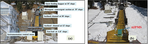
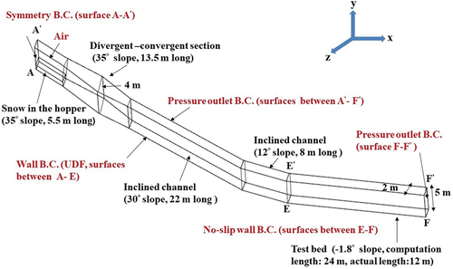
An avalanche impact pressure measurement system (AIPMS) was developed to measure the impact pressure of avalanches on a 61-m-long and 2-m-wide snow slide at Dhundhi, Himachal Pradesh, India. Dhundhi is located at an altitude of 3,030 m in the Pir Panjal range of Indian Himalaya. At this site, the average cumulative seasonal snowfall is about 11 m and the winter air temperature varies from a minimum of −15°C to a maximum of +10°C. The snow chute consists of five sections as shown in Figure 1a. The bottom surface of the chute is made of low-carbon steel sheets of thickness 12 mm. Each sheet is 2 m × 4 m for most sections of the chute. Transparent polycarbonate sheets are fitted in the side railing (1 m high) of the snow chute. Alternate colors are painted at 0.5-m intervals on the bottom surface of the chute for ease of measurement of the snow flow parameters. The angle of the hopper was kept fixed at 35°. The length of the hopper is 5.5 m and its maximum snow filling capacity, V, is 11 m³. At the end of the hopper, a 13.5-m-long diverging–converging channel inclined at 35° is provided to ensure fluidization of the snow. After this section, a 22-m-long channel inclined at 30° acts as an accelerating path for the snow that attains maximum velocity near the end of this channel. At the end of this section, an 8-m-long channel inclined at 12° is provided, which ensures a reduction in the momentum of snow flow. Finally, a 12-m-long test bed inclined at an angle of −1.8° is provided at the end, where the avalanche comes to a complete halt. The location of the AIPMS on the snow chute is shown in Figure 1b.

Figure 1. A view of the (a) snow chute at Dhundhi, Himachal Pradesh, India. (b) AIPMS on the test bed of the chute (at a distance of 0.9 m from the end of the 12° slope).

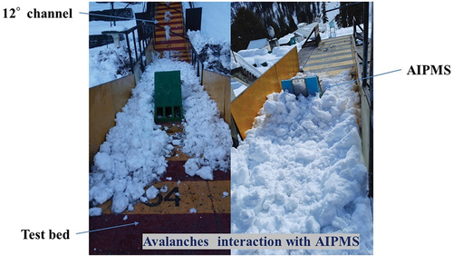
The AIPMS comprises four single-axis piezoelectric load cells fitted at an interval of 0.20 m on stainless steel plates of size 1 m × 0.25 m. Two plates each of 0.2 m width made from low-carbon steel were attached to the left and right sides of the steel plate. A schematic of the AIPMS is shown in Figure 2. The vertical load of the complete impact plate assembly is transferred to four reinforced concrete cement pillars through a 150-mm-thick low-carbon steel base frame. Further, the bending of the plate due to avalanche impact is resisted by a rigid low-carbon steel back support. Overall, the system is designed to measure a maximum 250 kPa avalanche impact pressure, P_m, with an accuracy of ±5.0 percent. To isolate the sensor assembly from the noise and vibrations from the snow chute body, a uniform gap of 10 mm was provided all around between the base frame and snow chute plates. The force sensors were calibrated in the laboratory by PCB Inc. Each load cell was capped with a circular-shaped steel shroud of area 314.28 mm². Neoprene washers were provided around each force sensor to prevent ingress of snow/moisture through the front plate of the impact assembly. In previous studies, impact pressure load cells with protruding surfaces were used (Jaedicke et al. 2008; Baroudi, Sovilla, and Thibert 2011; Sovilla et al. 2016). This arrangement of sensors may result in error in the pressure readings when large chunks of snow hit the sensor surface. In the present measurement system, to ensure that the force sensors measured avalanche impact force proportionate to its top surface area only, the top surfaces of the four force sensors were ground-flushed with the front plate of the assembly. The output of the four piezoelectric load cells was connected via four 20-m-long coaxial low-noise cables to a signal conditioner, which in turn was connected to a data acquisition system. Finally, the output of the data acquisition system was interfaced with a laptop for display, storage, and analysis of the data. The data sampling rate is 1,000 Hz. The complete assembly of the AIPMS is displayed in Figure 3. A closer view of the AIPMS and its interaction with the chute avalanches is shown in Figure 4.

Figure 2. Schematic of the AIPMS showing (a) its position at a distance of 0.9 m from the end of the 12° slope of the snow chute, (b) its front plate facing the avalanche, and (c) side view showing the back support detail.

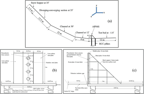
Figure 3. A view of the AIPMS installed on snow chute, Dhundhi, Himachal Pradesh, India.

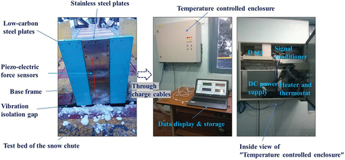
Figure 4. A view of the interaction of the snow avalanches with AIPMS at the snow chute, Dhundhi, Himachal Pradesh, India.

Model and simulations detail

Main governing equations

In the present work, avalanche flow modeling and its interaction with an instrumented obstacle was performed in the 3D domain. Both snow and air are considered incompressible in the model. The model mainly solves the multiphase equations for the snow and surrounding atmospheric air phases (Bovet et al. 2007). Here, phase means the unique state of matter such as solid or fluid. In the present case, both snow and air are taken as fluid phases. Brief details of the main flow governing equations are given in online appendix 1 (ANSYS Inc. 2015).

Discretization and numerical solution of the model

A control volume–based technique was used to convert the mass and momentum equations (A2) to (A3) (online appendix 1) to algebraic equations that can be solved numerically. This control volume technique consists of integrating the above transport equations about each control volume, yielding discrete equations that express the conservation law on a control volume basis. In the current work, a pressure-based transient solver was chosen, because a density-based solver is not compatible with multiphase flows. Pressure–velocity coupling was solved using the semi-implicit method for pressure-linked equations algorithm (Patankar 2009). For spatial discretization, a first-order upwind scheme was chosen in which the face value was set equal to the cell center value in the upstream cell. Because the mesh is hexahedral and aligned with the flow, selection of a first-order scheme is reasonable. For computation of the gradients, a least squares cell-based gradient approach was used in which the solution is assumed to vary linearly. A multifluid volume of fluid (VOF) model was used along with a Eulerian model for the interface sharpening between the snow and air phases (Hirt and Nichols 1981). For the explicit mode of computation of volume fraction of snow and air phases, a geometric reconstruction interpolation scheme was selected to enable a sharp interface between the phases. Further, the Geo-Reconstruct scheme ensures the time-accurate transient behavior of the VOF solution. For the transient part of the momentum equations, a first-order implicit formulation was selected.

Solver parameters for the simulations

The computation timestep ε for all simulations was uniformly taken as 0.001 second. The underrelaxation factors for the pressure, density, body forces, and momentum were taken as 0.3, 1.0, 1.0, and 0.7, respectively. The convergence criterion for the solution was set with a residual value of 0.001 for both continuity and momentum equations. The value of acceleration due to gravity $\vec{g}$ was taken as 9.81 m·s⁻². Then the equations were initialized, the snow phase was patched with a VOF value equal to 1.0, and the simulations were run. The solution for the various parameters (i.e., pressure, velocity, volume fraction, etc.) was automatically saved at regular intervals.

Domain, boundary conditions, and material properties

The 3D geometry of the snow chute was drawn in the ANSYS Workbench module by considering the total computation domain size as 73 m long, 2 m wide, and 5 m high as shown in Figure 5 (ANSYS Inc. 2015). It should be noted that the actual length of the snow chute is 61 m. The computation domain of the chute was considered longer than the actual size to contain the simulations beyond the run-out distance of 12 m. At the start of snow flow (A–A′), a symmetry boundary condition was applied; that is, a wall with zero shear stress. At the arbitrarily drawn top surface, which is open to the atmosphere, a pressure outlet boundary condition was applied. At the end section of the chute, a pressure outlet boundary condition was also applied. At the bottom surfaces of the snow chute except the test bed surface, a user-defined wall shear function was applied, details of which are provided next. At the test bed surface (E–F), a no-slip boundary condition was applied, because friction is maximum in the deceleration zone (Nishimura and Maeno 1989).

Figure 5. Boundary conditions for the 3D geometry of the snow chute at Dhundhi, Himachal Pradesh (Aggarwal and Kumar 2012).

Wall shear stress model

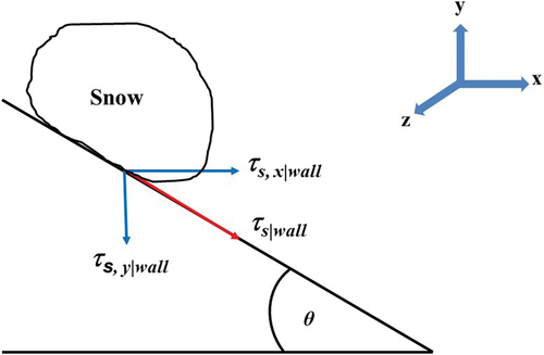
The no-slip boundary condition, in which the slip velocity is set to zero, has been widely and successfully used in many fluid flow simulations. However, a number of previous studies have proved that snow, as a granular material, moves with a slip velocity at the snow–ground interface (Bovet et al. 2007; Upadhyay, Kumar, and Chaudhary 2010; Domnik and Pudasaini 2012). An advanced model for the calculation of wall slip velocity was presented by Domnik and Pudasaini (2012). However, it was difficult to implement this model in the current code because it requires values of x- and y-components of the wall shear stress at the wall to replace the no-slip boundary condition. Therefore, in this article, a simple mathematical model accounting for wall slip in the x- and y-directions is presented. Taking the value of the wall shear stress in the z-direction as zero because the variation in avalanche flow parameters is predominantly in the x- and y-directions, total wall shear stress τ_s|wall (N·m⁻²) at the snow–chute bottom interface along the chute flow is given below (Figure 6):

(1) ${\tau }_{\mathit{s}|\mathrm{wall}}=\left(1-W_s\right){\eta }_s\left(\frac{\mathrm{\partial u}}{\mathrm{\partial y}}+\frac{\mathrm{\partial v}}{\mathrm{\partial x}}\right).$(1)

Figure 6. Wall shear stress components of snow on an inclined plane. τ_s|wall (N·m⁻²) stands for the total wall shear stress of snow, τ_s,x|wall (N·m⁻²) stands for the x-component of τ_s|wall, τ_{s, y|wall} (N·m⁻²) stands for the y-component of τ_s|wall, and θ (°) is the angle of the plane.

Here, W_s can be defined as the wall slip factor, whose value can vary from zero to one. The value of W_s = 0 implies minimum slip and maximum wall shear stress values. In case of a no-slip fluid wall condition, maximum wall shear stress is present. The Coulomb friction coefficient ξ can be computed as the ratio of the snow wall shear stress τ_s|wall and the snow hydrodynamic pressure p. Here, p =ρ_igh_s, where h_s is the simulated depth of the snow. Therefore, for a constant p value at a point, it can be deduced that maximum Coulomb friction exists whenever a maximum fluid wall shear stress condition is reached. Similarly, W_s = 1 corresponds to zero wall shear stress and can be termed as maximum slip or free-slip wall condition. In this case, Coulomb friction is also zero. Values of W_s between zero and one will determine the intermediate slip at the snow–chute bottom interface. Because the program code requires components of wall shear stress in x-, y-, and z-directions, resolving τ_s|wall into x- and y-components, the x-component of wall shear stress is given as

(2) ${\tau }_{\mathit{s},\mathit{x}|\mathrm{wall}}=\left(1-W_s\right)\mathit{\hspace{0.17em}}{\eta }_s\left(\frac{\mathrm{\partial u}}{\mathrm{\partial y}}+\frac{\mathrm{\partial v}}{\mathrm{\partial x}}\right)\mathit{cos\theta }\mathit{\hspace{0.17em}}.$(2)

Similarly, the y-component of the wall shear stress is given as

(3) ${\tau }_{\mathrm{s},\mathrm{y}|\mathrm{wall}}=-\left(1-W_s\right)\mathit{\hspace{0.17em}}{\eta }_{\mathrm{s}}\left(\frac{\mathrm{\partial }\mathit{u}}{\mathrm{\partial y}}+\frac{\mathrm{\partial v}}{\mathrm{\partial x}}\right)\sin \mathit{\theta }\mathit{\hspace{0.17em}}.$(3)

Here, θ is the angle of the slope. In the current work, for all model simulations, the value of W_s is taken as 0.25. With this value, the average value of the simulated dynamic Coulomb coefficient of friction between the snow chute steel surface and the snow ξ was estimated as 0.12. The simulated friction coefficient value is in agreement with the measurements by Aggarwal (2019), who obtained an average measured value of 0.11 for the dynamic Coulomb coefficient of friction between the snow chute steel surface and snow.

Physical properties of snow and air

The properties of air were taken as constant with a dynamic viscosity µ_a as 1.7894 × 10⁻⁵ N·s·m⁻² and density ρ_a as1.225 kg·m⁻³. Snow, which is a highly complex and dynamically changing material, was assumed to be a bi-viscous Bingham fluid. The constitutive equation of an ideal Bingham fluid is made up of two parts. First, if the shear stress intensity τ (N·m⁻²) is below a yield stress value τ₀ (N·m⁻²), no deformation takes place and the material behaves as a rigid solid. Second, if τ is above this value, deformation takes place and is proportional to the amount that τ exceeds τ₀ (Figure 7).

Figure 7. Flow rheology of snow as a bi-viscous Bingham fluid. τ₀ (N·m⁻²) stands for the yield strength of snow, ${\eta }_0$ (N·s·m⁻²) stands for the dynamic viscosity of snow in the locked portion of the flow, k (N·s·m⁻²) stands for the dynamic viscosity of snow after the yield region, and ${\dot{\gamma }}_0$ (s⁻¹) stands for the shear strain rate of snow in the locked portion of the flow.

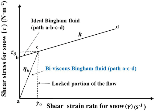
This model is difficult to implement because of sharp discontinuity at τ = τ₀. To rectify this anomaly, in this article, the bi-viscous Bingham fluid model was adopted from Dent and Lang (1983), which allows small deformations to take place according to a linear viscous flow law in the locked portion of the flow as shown by a dotted line in Figure 7. The dynamic viscosity ${\eta }_0$ used in this region is assumed as 10⁴ N·s·m⁻². This value is taken significantly high so that the resulting deformation can be neglected relative to the deformation outside this region (Oda et al. 2011). Following the work of Dent and Lang (1983), Alexandrou et al. (2003), and Oda et al. (2011), the effective Newtonian viscosity of snow, ${\eta }_{\mathrm{s}}$, for a bi-viscous Bingham fluid can be written as

(4) ${\eta }_{\mathrm{s}}=\frac{{\tau }_0}{\dot{\gamma }}+\mathit{k}\left(1-\frac{{\dot{\gamma }}_0}{\dot{\gamma }}\right),$(4)

where $\mathit{\gamma }$ (s⁻¹) is the shear strain rate after the yield region. k (N·s·m⁻²) is the dynamic viscosity coefficient of snow after the yield region. In the present work, the value of k was taken as 0.02 N·s·m⁻² for all simulations (Domnik and Pudasaini 2012). This value is justified because snow flows like a Newtonian fluid with quite low viscosity after the yield region. Here, ${\dot{\gamma }}_0$ (s⁻¹) is the strain rate in the locked flow regime, which is computed as

(5) ${\dot{\gamma }}_0=\frac{{\tau }_0}{{\eta }_0}\mathit{\hspace{0.17em}}.$(5)

The yield strength of snow, τ₀, is the function of hydrodynamic pressure p, cohesion strength c, and internal friction angle of snow φ, as written below (Oda et al. 2011):

(6) ${\tau }_0=\mathit{c}+\mathit{p}\tan \mathit{\phi }.$(6)

In the current work, cohesion c between snow grains is neglected. Substituting Equation (5)(5) ${\dot{\gamma }}_0=\frac{{\tau }_0}{{\eta }_0}\mathit{\hspace{0.17em}}.$(5) and Equation (6)(6) ${\tau }_0=\mathit{c}+\mathit{p}\tan \mathit{\phi }.$(6) into Equation (4)(4) ${\eta }_{\mathrm{s}}=\frac{{\tau }_0}{\dot{\gamma }}+\mathit{k}\left(1-\frac{{\dot{\gamma }}_0}{\dot{\gamma }}\right),$(4) , ${\eta }_{\mathrm{s}}$ can be rewritten as

(7) ${\eta }_{\mathrm{s}}=\frac{\mathit{p}\tan \phi }{\dot{\gamma }}+\mathit{k}\left(1-\frac{{\dot{\gamma }}_0}{\dot{\gamma }}\right).$(7)

$\mathit{\gamma }$ $\dot{\gamma }$ is related to the second invariant of the rate of the deformation tensor, $\overline{\stackrel{‾}{D}}$, as

(8) $\dot{\gamma }=\sqrt{\frac{1}{2}\mathit{\hspace{0.17em}}\overline{\stackrel{‾}{D}}:\overline{\stackrel{‾}{D}}\mathit{\hspace{0.17em}}}.$(8)

Here, $\overline{\overline{D}}=\nabla {\overrightarrow{v}}_{\mathit{s}}+\nabla {\overrightarrow{v}}_{\mathit{s}}^{\mathit{T}}$.

On simplification and algebraic manipulation, Equation (8)(8) $\dot{\gamma }=\sqrt{\frac{1}{2}\mathit{\hspace{0.17em}}\overline{\stackrel{‾}{D}}:\overline{\stackrel{‾}{D}}\mathit{\hspace{0.17em}}}.$(8) reduces to

(9) $\mathit{\hspace{0.17em}}{\dot{\gamma }}^2=2{\left(\frac{\mathrm{\partial u}}{\mathrm{\partial x}}\right)}^2+2{\left(\frac{\mathrm{\partial v}}{\mathrm{\partial y}}\right)}^2+\frac{\mathrm{\partial u}}{\mathrm{\partial y}}\left(\frac{\mathrm{\partial u}}{\mathrm{\partial y}}+\frac{\mathrm{\partial v}}{\mathrm{\partial x}}\right)+\frac{\mathrm{\partial v}}{\mathrm{\partial x}}\left(\frac{\mathrm{\partial v}}{\mathrm{\partial x}}+\frac{\mathrm{\partial u}}{\mathrm{\partial y}}\right)$(9)

where u and v are the velocities in the x- and y-directions, respectively. A user-defined function was written for the above viscosity model and hooked to the main program code (Equation (7)(7) ${\eta }_{\mathrm{s}}=\frac{\mathit{p}\tan \phi }{\dot{\gamma }}+\mathit{k}\left(1-\frac{{\dot{\gamma }}_0}{\dot{\gamma }}\right).$(7) ).

Recently, based on a large number of measurements, Aggarwal (2022) published a correlation between the density of snow ρ_i (kg·m⁻³) and the angle of repose of snow β (°). Equation (10)(10) $\mathit{\beta }=-13.24\mathit{ln}\left({\rho }_i\right)+117.69\mathit{\hspace{0.17em}}.$(10) developed in this work was used to estimate the angle of repose of snow for different densities of snow noted in the experiments:

(10) $\mathit{\beta }=-13.24\mathit{ln}\left({\rho }_i\right)+117.69\mathit{\hspace{0.17em}}.$(10)

For granular cohesionless snow, the angle of repose of snow, β, is essentially the same as its internal friction angle φ (Al-Hashemi and Al-Amoudi 2018). With this assumption, the internal friction angle of snow φ was estimated.

Mesh size dependence

The simulations were run using 48 GB RAM and two Intel Xenon CPU [email protected] GHz processors (each processor had six cores). The program code was enabled to utilize the ten cores of the workstation in the parallel computing mode. One of the simulations (15 March 2021; experiment E2) was selected to determine the optimum mesh size for the simulations. First, a hex mesh of size 0.025 m was chosen for the mesh generation, which could not be generated due to dynamic memory allocation error. Then the mesh size was increased to 0.05 m, 0.1 m, etc. Next, keeping the computation timestep ε and all other parameters identical, the simulations were run for the different mesh sizes. For reference, comparison between the simulated snow velocity v_s contours for the three mesh sizes at a flow timestep t =1.5 s is given in Figures 8a-c. Complete information on effects of different mesh sizes is given in Table 2. From Table 2, it is clear that with an increase in mesh size, there is decrease in the computation time but a simultaneous increase in the deviation in the simulated maximum snow velocity v_s,max values with respect to the mesh size of 0.05 m. Further, it can be seen that there is a significant deviation between the computation flow time for the 0.05-m mesh size and others but the deviation between the v_s,max values and the deformation pattern for 0.05- and 0.1-m mesh sizes is not very significant. Therefore, as a trade-off between accuracy and computation time, a mesh size of 0.1 m was chosen for all simulations reported in this article.

Figure 8. Contours of snow velocity v_S at a timestep t = 1.5 seconds, after the release of 11 m³ of snow of density ρ_i = 582 kg·m⁻³ from the hopper of the snow chute, Dhundhi, Himachal Pradesh, India, for the varying mesh sizes of (a) 0.05 m, (b) 0.1 m, and (c) 0.2 m (15 March 2021; experiment E2).

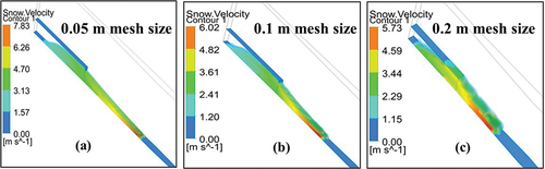
Table 2. Effect of the mesh size on the model simulations.

Mesh size (m)	Maximum aspect ratio	Minimum orthogonal quality	Number of cells	Time taken to complete 1.5-second simulation (hours)	Estimated time taken to complete the full simulation (hours)	Simulated max. snow velocity vs,max at t = 1.5 seconds (m· s^−1)
0.025	Memory allocation error while generating the mesh
0.050	3.3220	0.8106	5,792,000	60.39	322.09	7.83
0.10	3.3205	0.8110	724,000	1.54	8.22	6.02
0.20	3.3169	0.8118	90,750	0.60	3.20	5.73

Results and discussion

As shown in Table 3, a total of seven experiments were performed during the period 2020 to 2021 on the AIPMS to measure avalanche impact pressure, P_m, values. For the experiments, undisturbed snow was manually filled in the hopper from the surrounding area. Minor compaction of the snow occurred during the experiments owing to shoveling of snow into the hopper. Before opening the gate of the hopper, snow temperature T_s(°C) and density ρ_i (kg·m⁻³) were noted at the bottom, middle, and top portions of the hopper. These values of T_s and ρ_i were averaged before use in the computations.

Table 3. Summary of the experiments for the measurement of avalanche impact pressure P_m at the snow chute, Dhundhi, Himachal Pradesh, India.

Date of experiment	Volume of snow in the hopper, V (m^3)	Average density of snow in the hopper, ρi (kg·m^−3)	Average density of snow near AIPMS after hitting, ρf (kg ·m^−3)	Types of snow grains	ISCG^a code	Liquid water content in the snow	Average temperature of snow, Ts (°C)	Natural/sieved snow
14 February 2020	11	325	445	Rounded grains	RGlr	M	−1.0	Natural
17 February 2020	11	415	550	Melt forms	MFcl	M	−0.5	Natural
23 February 2020	11	445	545	Melt forms	MFcl	M	−0.5	Natural
15 March 2021 (E1)	11	578	635	Melt forms	MFcl	M	0.2	Natural
15 March 2021 (E2)	11	582	640	Melt forms	MFcl	M	0.2	Natural
18 March 2021	11	565	602	Melt forms	MFcl	M	−0.3	Natural
19 March 2021	11	542	576	Melt forms	MFcl	M	0.4	Natural

Note: ^aThe International Classification for Seasonal Snow on the Ground (Fierz et al. 2009).

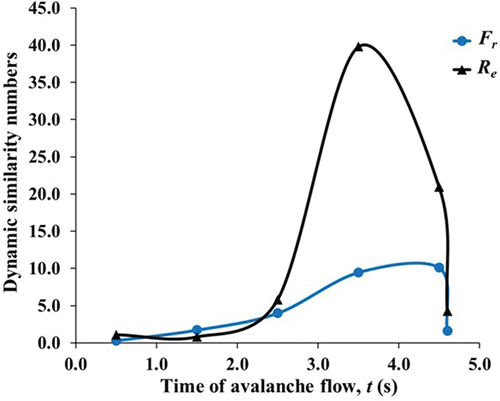
The phenomenon of snow avalanches is gravity driven. Dimensional analysis indicates that the law of similitude requires the Froude number $F_r=v_s/v_s\sqrt{\mathit{g}{h}_s}-\sqrt{\mathit{g}{h}_s}$ of the flow to be invariant under transformations to the laboratory scale. The F_r exhibited by the flow as shown in Figure 9 was in the range 8 to 10, which almost overlaps with the range of F_r exhibited by the real-scale avalanches, thereby ensureing a dynamic similarity between the experimental runs and natural snow avalanches (Sheikh, Verma, and Kumar 2008). Lang and Dent (1980) showed that small-scale modeling of snow avalanches is feasible for the geometric, kinematic, and dynamic similarity based upon the numerical equivalence of the Froude number F_r between the prototype and model avalanches. The authors obtained a Froude number value of 9.6 for the prototype avalanche and 11.2 for the small-scale avalanche. However, this similarity of F_r between the real- and small-scale avalanches may not hold for the complete spectrum of the avalanches and does not prove that the similarity is due to the same underlying effects (Sovilla, Schaer et al. 2008). In the current work, as shown in Figure 9, the Reynolds number, R_e, of the avalanche flow varied from 20 to 39. Therefore, the avalanche in the chute channel (and simulated by the presented numerical model) is a fast laminar flow.

Figure 9. Variation of simulated Reynolds number R_e and Froude number F_r of the flowing snow shown as a function of time t, just after the snow is released from the hopper of the snow chute, Dhundhi, Himachal Pradesh, India, for the demonstration of the dynamic behavior of the chute avalanches versus real avalanches.

In Figure 10, the flow of simulated avalanche mass and its interaction with AIPMS at various flow timesteps t is shown. Contours of snow velocity v_s are shown in Figure 11a for a timestep t =5.2 s. It can be seen from Figure 11a that the frontal velocity of the avalanche flow becomes zero the moment it hits the instrumented structure and most of its dynamic pressure P_d is converted to the hydrodynamic pressure p. The contours of the snow total pressure P_s are shown in Figure 11b. P_s is the sum of P_d and p; that is, $P_s=1/12-{\rho }_i{v}_s^2+\mathit{p}$. It is clarified here that snow total pressure is the same as the simulated avalanche impact pressure. The observed flow of the avalanche mass at various timesteps t during the experiment conducted on 17 February 2020 is shown in Figure 12. On comparing the simulated avalanche snow depths h_s with experimentally observed snow depths h_e at the specific points marked in Figures 10 and 12, it was found that both values were on the same order. Figures 13 and 14 show a comparison between the instantaneous measured P_m and simulated avalanche impact pressures P_s at 0.2 m depth and 0.6 depth of the AIPMS. In most of the experiments reported in this work, snow did not touch the force sensor located at 0.8 m depth of the AIPMS and so only extreme variation of pressures at 0.2 and 0.6 m depths is reported. In all of these experiments, the avalanche could flow from the sides of the AIPMS as shown in Figures 1 and 4. It can be seen that there were significant deviations between the P_m and P_s values as depicted by root mean square error (RMSE), ranging from 5.26 to 18.93. In a few cases, there was also a time lag between the P_m and P_s values. In almost all cases reported, there were fluctuations in the P_m values for a short duration, whereas P_s values remain nearly constant for a longer duration of time. The main reason for these deviations was the dominance of granular solid behavior of snow in the observed snow chute avalanches in comparison to the dominant fluid behavior in the simulated chute avalanches. Because moist snow was used in the experiments, it is also possible that in some cases large chunks of nonfluidized snow may have hit the impact sensors, resulting in large pressure values. Further, compressibility of snow is another possible reason for the much larger P_m values than the P_s ones (Eglit, Kulibaba, and Naaim 2007). A a large snow mass deposits in front of the impact pressure sensors, exerting higher impact pressures as compared to the simulatations, in which a large avalanche mass passes around the AIPMS structure (Caccamo et al. 2011; Faug, Caccamo, and Chanut 2012). Another reason for high fluctuations in the measured pressure values is the high sampling rate of 1,000 Hz at which the data were acquired. To assess the reasons for the deviations between the P_m and P_s values, a comparison was drawn between the peak measured pressure P_m,max values and the corresponding peak simulated pressure values P_s,max values at 0.2 m depth as shown in Table 4. Because P_m,max values were observed at the bottom-most part of the AIPMS, only values at 0.2-m depth are shown in Table 4. On quantitative analysis, it can be seen that ratio R_p between P_m,max and P_s,max values steadily increased with an increase in the initial density of snow, ρ_i, which was expected because with an increase in ρ_i, the solid behavior of the snow increases, which was only partly accounted for in the simulations. The average value of this ratio R_p was 2.94, which means that P_m,max values are roughly three times higher than the P_s,max values. It is obvious that the present simulations consider the incompressible snow density effects in the results and thus are able to capture only approximate dynamic behavior of the avalanches. However, in the measurements, snow microscopic properties like grain cohesion, formation of network of grain chains, snow block formation due to moisture, and compressibility of snow interact in a complex manner. Therefore, there was also a time lag between the P_s,max and P_m,max values. Despite all of these limitations, we propose using the ratio R_p for the further approximate analysis of the results.

Figure 10. Simulation results of experiment on 17 February 2020 for avalanche flow mass and its interaction with AIPMS at various timesteps t of the flow.

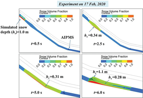
Figure 11. At a timestep t =5.2 s, simulated (a) snow velocity v_s and (b) snow total pressure (impact pressure) P_s (17 February 2020).

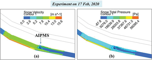
Figure 12. Observation of the avalanche flow and its depth at the significant points on the snow chute at various flow timesteps t during the experiment carried out on 17 February 2020.

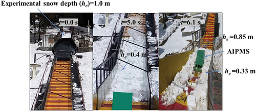
Figure 13. Simulated versus measured avalanche impact pressures at (a) 0.2-m and (b) 0.6-m depth from the snow chute test bed surface (14 February 2020, 17 February 2020, and 23 February 2020).

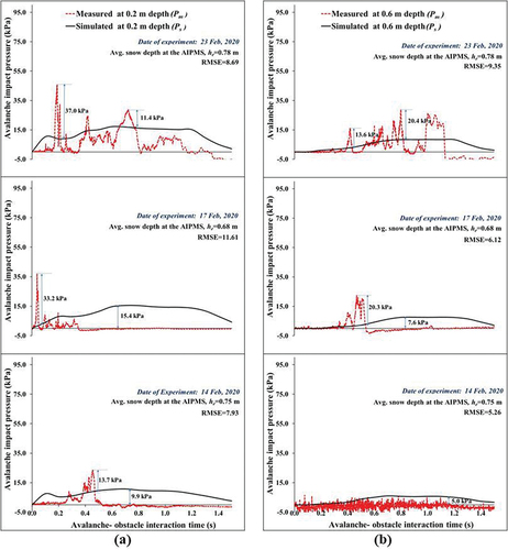
Figure 14. Simulated versus measured avalanche impact pressures at (a) 0.2-m depth and (b) 0.6-m depth from the snow chute test bed surface (15 March 2021, experiment E1; 18 March 2021; and 19 March 2021).

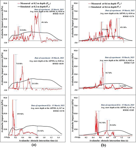
Table 4. Ratio R_p of the peak values of the measured avalanche impact pressures P_m,max and simulated avalanche impact pressures P_s,max.

Sr. no.	Average density of snow before impact, ρi (kg· m^−3)	Peak value of the simulated impact pressure, Ps,max (kPa)	Peak value of the measured impact pressure, Pm,max (kPa)	$\mathrm{Ratio}{R}_p=\frac{\mathit{P}{\mathit{ }}_{\mathit{m},\mathit{max}}}{\mathit{P}{ }_{\mathit{s},\mathit{max}}}$
1.	325	10.77	23.60	2.19
2.	415	15.45	37.20	2.41
3.	445	17.23	46.00	2.67
4.	542	22.59	71.90	3.18
5.	565	24.20	84.90	3.51
6.	578	24.57	90.26	3.67

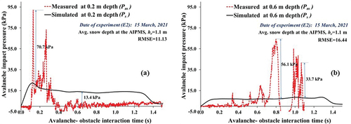
In Figure 15, the avalanche flow interaction with AIPMS is shown when the flow is completely blocked from both sides (15 March 2021; experiment E2). For this case, a comparison between the P_m and P_s values is shown in Figure 16. In this case, it can be seen that P_m values are similar to the case when the flow was open from the sides. The peak P_s,max value is also similar to the case when the flow was open from the sides of the AIPMS. However, the P_s values remain on the higher side for a much longer time on the structure. This is due to the blocking of the snow. The main mechanism for higher P_m values in case of high-density moist snow avalanches is the large-sized blocks of snow hitting the structure. Thus, in case of high-density avalanches, the confinement or unconfinement of the flow does not seem to play significant role in affecting the impact pressure values (Figure 16).

Figure 15. Measurement of the avalanche impact pressures P_m by AIPMS after complete blocking of the avalanche flow from the sides with barriers (15 March 2021, experiment E2).

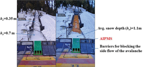
Figure 16. Simulated versus measured avalanche impact pressures after complete blocking of flow from the sides with the barriers at (a) 0.2-m depth and (b) 0.6-m depth from the snow chute test bed surface (15 March 2021, experiment E2).

Estimation of the fluid drag coefficient C_d and the effective drag coefficient $C_d^{\prime }$

The fluid drag coefficient C_d for the snow and obstacle was estimated from the following equation (Som and Biswas 2008):

(11) $C_{\mathit{d}\mathit{\hspace{0.17em}}}=\frac{F_d}{\frac{1}{2}\mathit{\hspace{0.17em}}{\rho }_{\mathit{i}\mathit{\hspace{0.17em}}}{A}_{\mathit{p}\mathit{\hspace{0.17em}}}{v}_{sf}^2}.$(11)

Here, F_d (N) is the drag force computed on the frontal projected area A_p of the AIPMS, which is computed as the summation of pressure force over the obstacle faces; that is, $F_{\mathit{d}}=\sum _{\mathit{i}=1}^n{p}_{\mathit{i}}{A}_i$. In the present case, the value of A_p is computed as 0.65 m², and v_sf (m·s⁻¹) is the average free-stream snow velocity; that is, the velocity far away from the obstacle. It can be seen from Equation (11)(11) $C_{\mathit{d}\mathit{\hspace{0.17em}}}=\frac{F_d}{\frac{1}{2}\mathit{\hspace{0.17em}}{\rho }_{\mathit{i}\mathit{\hspace{0.17em}}}{A}_{\mathit{p}\mathit{\hspace{0.17em}}}{v}_{sf}^2}.$(11) that the value of v_sf should be known in advance for the estimation of C_d for the varying value of the drag force F_d. Therefore, to estimate v_sf, snow velocity v_s was noted at a flow time interval t = 0.1 s during the avalanche–AIPMS interaction process at an 0.8-m distance from the center of the AIPMS in the z-direction at a depth of 0.4 m from the snow chute surface and the values obtained were averaged. Then the simulation was rerun for the avalanche–AIPMS interaction process by feeding the required value of v_sf, obtained from the initial simulation in Equation (11)(11) $C_{\mathit{d}\mathit{\hspace{0.17em}}}=\frac{F_d}{\frac{1}{2}\mathit{\hspace{0.17em}}{\rho }_{\mathit{i}\mathit{\hspace{0.17em}}}{A}_{\mathit{p}\mathit{\hspace{0.17em}}}{v}_{sf}^2}.$(11) and results for the drag coefficient C_d obtained, as shown in Figures 17a-b. From this figure, it is clear that initially the values of C_d increased with flow time as F_d increased on the obstacle, remained constant for some time, and finally decreased toward zero. It can be further observed that the maximum value of C_d was almost double in case of ρ_i =325 kg·m⁻³ compared to ρ_i = 578 kg·m⁻³. Further, the average value of C_d was estimated as 1.35 for ρ_i = 578 kg·m⁻³ and 2.90 for ρ_i = 325 kg·m⁻³. This result shows that in case of slower-moving avalanches, the value of C_d is higher than that for fast-moving avalanches. In the present case, the average value of C_d considering both the extreme cases is ≈2.13. However, as noted, there was a strong deviation between the P_s and the P_m values. This means that C_d is not sufficient to account for the deviations between the two values. The concept of C_d is borrowed from the fluid mechanics theories. However, snow in the form of an avalanche has both fluid and solid granular properties, which jointly affect the values of the avalanche impact pressure on the obstacles. To take into account the solid, granular, and compressibility effects of snow, we propose that peak avalanche impact pressure P_i for a dense flow of avalanche on any structure in the avalanche path can be estimated from the following equation:

(12) $P_i=\frac{1}{2}\mathit{\hspace{0.17em}}{C}_d^{\prime }{\rho }_i\mathit{\hspace{0.17em}}{v}_{sf}^2$(12)

Figure 17. Variation of simulated fluid drag coefficient C_d and the corresponding effective drag coefficient $C_d^{\prime }$ during the avalanche flow–obstacle interaction process for experiments conducted on (a) 15 March 2021 (experiment E1, ρ_i = 578 kg·m⁻³) and (b) 14 February 2020 (ρ_i = 325 kg·m⁻³).

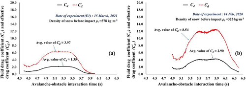
$C_d^{\prime }$ is the effective drag coefficient, which can be considered ~R_p C_d.

Alternatively, P_i can be estimated as $P_i=R_p{P}_{\mathit{s},\mathit{max}}$. Values of $C_d^{\prime }$ are also plotted in Figures 17a and 17b. It can be observed that, essentially, the variation trend of C_d and $C_d^{\prime }$ values remains the same. These results are in agreement with the works of Naaim et al. (2008) and Sovilla, Schaer et al. (2008), who obtained lower values of $C_d^{\prime }$ with increasing F_r. Further, the network of chain forces formed inside the dead zone might lead to enhancement of drag coefficients in low-velocity regimes (Faug, Caccamo, and Chanut 2012). Our deductions are also in agreement with the recent work of Kyburz et al. (2022), who considered the effective drag coefficient $C_d^{\prime }$ as the product of an obstacle geometry factor and a flow regime factor. In the flow regime factor, the authors considered solid, granular, and fluid properties of the snow. However, most previous research has used $C_d^{\prime }$ values for estimating avalanche impact pressures without modeling the actual structure–avalanche interaction process. In the present case, average $C_d^{\prime }$ values varied from nearly 3.97 to 8.54. This range of values is in agreement with the deductions of Salway (1978), who, based on limited field measurements, obtain drag coefficient values in the range of ≈4 to 12. Our results are also in concordance with Sovilla et al. (2016), who accounted for the huge impact pressure values by fitting large C_d and ζ values for the dynamic pressure component and the hydrodynamic pressure component, respectively.

Comparison of current model with the other models

The peak pressures obtained in the current simulations and measurements were compared with existing models to understand the scatter in the different models. We emphasize the use of peak avalanche impact pressure values for the design of safe avalanche control structures, in agreement with the observations of Eglit, Kulibaba, and Naaim (2007). A comparison between the output of present proposed model P_i and a few prominent models for the estimation of peak avalanche impact pressures is shown in Figure 18. The numerical values for the model comparisons are given in Table A1 in online appendix 2. It should be noted that in all of the abovementioned models (Voellmy 1955; Furukawa 1957; Sovilla et al. 2016), the velocity of the block of snow, v_s, was estimated from the Voellmy-Salm model as 8.52 m·s⁻¹. For details of the model computation, the reader can refer to Verma et al. (2004). Further, for the impact pressure calculation in the Voellmy model, a drag coefficient C_d value of 2.13 was used.

Figure 18. Comparison of deviations between the output of the proposed model P_i and other well-known models for the estimation of peak avalanche impact pressures on the obstacles. Deviations for the above models were calculated with reference to the peak measured avalanche impact pressures P_m,max in the current experiments.

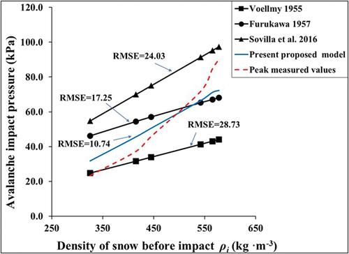
From the results, it is clear that there are significant deviations between P_m,max and P_s,max values estimated by various empirical models. This demonstrates that the hydraulics-based models can give only rough estimates for the avalanche impact pressure values. However, there is minimum RMSE ≈ 10.74 between the output of the present proposed model’s P_i and P_m,max values, which indicates that the proposed model has better capability than existing models. To further improve the direct agreement between the model and measurements, snow microstructural properties like porosity, cohesion, moisture content, etc., along with the compressibility of snow need to be incorporated in future models.

Conclusions

One locally developed experimental facility was used to measure the transient variation in avalanche impact pressures. To obtain a broad understanding of the subject, measured impact pressures were compared with the simulated values obtained through a 3D Navier-Stokes equations–based model. Most existing studies have used 2D models for the simulation of avalanche flow parameters. However, the present 3D model captured the realistic avalanche flow–structure interaction process with minimal assumptions. The deviations between the measured and simulated avalanche impact pressures for the dense flow of avalanches was accounted for. The RMSE between the present proposed model and the measured data was found a minimum (i.e., nearly 10.74) compared to existing prominent models for the estimation of avalanche impact pressure. Further, it was found that the fluid drag coefficient C_d alone is not sufficient to simulate the avalanche impact pressure on an obstacle in the avalanche’s path. However, the proposed effective drag coefficient $C_d^{\prime }$ was found to vary in the range of 3.97 to 8.54, which takes into account the solid, granular, and compressible properties of the snow and can better account for the deviations between the simulated and measured avalanche impact pressures. The present model can be easily extended for the simulation of avalanche impact pressures and related parameters in real mountain terrain. Therefore, the present study can provide useful inputs for improving the design guidelines for the middle zone and run-out zone avalanche control structures in mountainous areas. However, there is scope for further improvement. If snow is modeled as a granular multiphase material with cohesive, compressible properties in place of a continuum incompressible fluid, the model results can be greatly improved.

Acknowledgments

The authors are grateful to the Director, Defence Geoinformatics Research Establishment (DGRE), Chandigarh, for his kind support and motivation in carrying out this task. Technical support of Shri Rakesh Kumar and Shri Ashwani Kumar in carrying out the field experiments is duly acknowledged here. Finally, the authors are grateful to IIT Ropar, Punjab, for the use of other facilities.

Disclosure statement

No potential conflict of interest was reported by the authors.

Supplementary material

Supplemental data for this article can be accessed online at https://doi.org/10.1080/15230430.2024.2302836

Additional information

Funding

This research received no specific grant from any funding agency in the public, commercial, or not-for-profit sectors.

References

- Aggarwal, R. K., 2019. New database for the estimation of dynamic coefficient of friction of snow. International Symposium on Snow Avalanches & Mitigation strategies (SAMS): 7–20 July, Chandigarh, India.
- Aggarwal, R. K. 2022. New experimental investigation into the angle of repose of snow. Journal of Cold Regions Engineering 36, no. 2: 06022002. doi:10.1061/(ASCE)CR1943-54950000276.
- Aggarwal, R. K., and A. Kumar. 2012. 2-D computational fluid dynamics model for avalanche flow interaction with an obstacle for snow chute at Dhundhi. International Symposium on Cryosphere and Climate Change (ISCCC): 2-4 April, Manali, India.
- Alexandrou, A. N., P. L. Mennb, G. Georgiou, and V. Entov. 2003. Flow instabilities of Herschel–Bulkley fluids. Journal of Non-Newtonian Fluid Mechanics 116: 19–32. doi:10.1016/S0377-0257(03)00113-7.
- Al-Hashemi, H. M., and O. Al-Amoudi. 2018. A review on the angle of repose of granular materials. Powder Technology 330: 397–417. doi:10.1016/j.powtec.2018.02.003.
- ANSYS Inc. 2015. User manual of ANSYS Fluent 15.0 software. Southpointe 275, Technology Drive, Canonsburg, USA.
- Baroudi, D., B. Sovilla, and E. Thibert. 2011. Effects of flow regime and sensor geometry on snow avalanche impact-pressure measurements. Journal of Glaciology 57, no. 202: 277–88. doi:10.3189/002214311796405988.
- Baroudi, D., and E. Thibert. 2009. An instrumented structure to measure avalanche impact pressure: Error analysis from Monte Carlo simulations. Cold Regions Science and Technology 59, no. 2–3: 242–50. doi:10.1016/j.coldregions.2009.05.010.
- Bovet, E., B. Chiaia, V. de Biagi, and B. Frigo. 2011. Pressure of snow avalanches against buildings. Applied Mechanics and Materials 82: 392–7. doi:10.4028/www.scientific.net/AMM.82.392.
- Bovet, E., B. Chiaia, and L. Preziosi. 2010. A new model for snow avalanche dynamics based on non-Newtonian fluids. Meccanica 45, no. 6: 753–65. doi:10.1007/s11012-009-9278-z.
- Bovet, E., B. Chiaia, L. Preziosi, and F. Barpi. 2007. The level set method applied to avalanches. Excerpt from the Proceedings of the COMSOL Users Conference: 23-24 October, Grenoble, France.
- Caccamo, P., T. Faug, H. Bellot, and F. Naaim-Bouvet. 2011. Experiments on a dry granular avalanche impacting an obstacle: Dead zone, granular jump and induced forces. WIT Transactions on the Built Environment 115: 53–62. doi:10.2495/FSI110061.
- Christen, M., J. Kowalski, and P. Bartelt. 2010. RAMMS: Numerical simulation of dense snow avalanches in three-dimensional terrain. Cold Regions Science and Technology 63, no. 1–2: 1–14. doi:10.1016/j.coldregions.2010.04.005.
- de Biagi, V., B. Chiaia, and B. Frigo. 2015. Impact of snow avalanche on buildings: Forces estimation from structural back-analyses. Engineering Structures 92, no. 1: 15–28. doi:10.1016/j.engstruct.2015.03.004.
- Dent, J. D., and T. E. Lang. 1983. A biviscous modified Bingham model of snow avalanche motion. Annals of Glaciology 4: 42–6. doi:10.3189/S0260305500005218.
- Domnik, B., and S. P. Pudasaini. 2012. Full two-dimensional rapid chute flows of simple viscoplastic granular materials with a pressure-dependent dynamic slip-velocity and their numerical simulations. Journal of Non-Newtonian Fluid Mechanics 173–174: 72–86. doi:10.1016/j.jnnfm.2012.03.001.
- Eglit, M. E., V. S. Kulibaba, and M. Naaim. 2007. Impact of a snow avalanche against an obstacle: Formation of shock waves. Cold Regions Science and Technology 50, no. 1–3: 86–96. doi:10.1016/j.coldregions.2007.06.005.
- Faug, T., P. Caccamo, and B. Chanut. 2012. A scaling law for impact force of a granular avalanche flowing past a wall. Geophysical Research Letters 39, no. 23: L23401(1–5). doi:10.1029/2012GL054112.
- Faug, T., B. Chanut, R. Beguin, M. Naaim, E. Thibert, and D. Baroudi. 2010. A simple analytical model for pressure on obstacles induced by snow avalanches. Annals of Glaciology 51, no. 54: 1–8. doi:10.3189/172756410791386481.
- Fierz, C., R. L. Armstrong, Y. Durand, P. Etchevers, E. Greene, D. M. McClung, K. Nishimura, P. K. Satyawali, and S. A. Sokratov. 2009. The international classification for seasonal snow on the ground. In IHP-VII Technical Documents in Hydrology N°83, IACS Contribution N°1. Paris: UNESCO-IHP.
- Frigo, B., P. Bartelt, B. Chiaia, I. Chiambretti, and M. Maggioni. 2020. Reverse dynamical investigation of the catastrophic wood-snow avalanche of 18 January 2017 at Rigopiano, Gran Sasso National Park, Italy. International Journal of Disaster Risk Science 12, no. 1: 40–55. doi: 10.1007/s13753-020-00306-6.
- Furukawa, I. 1957. Impact of avalanche. Journal of the Japanese Society of Snow and Ice 19 no, 5: 140–1. doi:10.5331/seppyo.19.140.
- Hauksson, S., M. Pagliardi, M. Barbolini, and T. Johannesson. 2007. Laboratory measurements of impact forces of supercritical granular flow against mast-like obstacles. Cold Regions Science and Technology 49, no. 1: 54–63. doi:10.1016/j.coldregions.2007.01.007.
- Hirt, C. W., and B. D. Nichols. 1981. Volume of Fluid (VOF) method for the dynamics of free boundaries. Journal of Computational Physics 39, no. 1: 201–25. doi:10.1016/0021-9991(81)90145-5.
- Jaedicke, C., M. A. Kern, P. Gauer, M. A. Baillifard, and K. Platzer. 2008. Chute experiments on slushflow dynamics. Cold Regions Science and Technology 51, no. 2–3: 156–67. doi:10.1016/j.coldregions.2007.03.011.
- Khapayev, S. A. 1978. Dynamics of avalanche natural complexes: An example from the high-mountain Teberda State Reserve, Caucasus Mountains, USSR. Arctic and Alpine Research 10, no. 2: 335–44. doi:10.2307/1550765.
- Kyburz, M. L., B. Sovilla, J. Gaume, and C. Ancey. 2022. Physics-based estimates of drag coefficients for the impact pressure calculation of dense snow avalanches. Engineering Structures 254, no. 1–17: 113478. doi:10.1016/j.engstruct.2021.113478.
- Lang, T. E., and J. D. Dent. 1980. Scale modeling of snow-avalanche impact on structures. Journal of Glaciology 26, no. 94: 189–96. doi:10.3189/S0022143000010728.
- Maggioni, M., M. Barbero, F. Barpi, M. Borri-Brunetto, V. de Biagi, M. Freppaz, B. Frigo, O. Pallara, and B. Chiaia. 2019. Snow avalanche impact measurements at the Seehore Test Site in Aosta Valley (NW Italian Alps). Geosciences 9, no. 471: 1–20. doi:10.3390/geosciences9110471.
- McClung, D. M., and P. Schaerer. 1999. The avalanche handbook. The Mountaineers, Seattle, Washington, USA.
- McClung, D. M., and P. A. Schaerer. 1985. Characteristics of flowing snow and avalanche impact pressures. Annals of Glaciology 6: 9–14. doi:10.3189/1985AoG6-1-9-14.
- Mead, L. B., H. Nakamura, T. E. Lang, and J. D. Dent. 1986. Comparison of experimental and computer modeling of snow-block impact on structures. Journal of Glaciology 32, no. 112: 321–4. doi:10.3189/S0022143000011989.
- Naaim, M., T. Faug, E. Thibert, N. Eckert, G. Chambon, F. Naaim, and H. Bellot. 2008. Snow avalanche pressure on obstacles. International Snow Science Workshop, 21–27 September, Whistler, B.C., Canada.
- Nakamura, T. 1987. A newly designed chute for snow avalanche experiments. International Association of Hydrological Sciences (IAHS) Publication 162: 441–51.
- Nishimura, K., and N. Maeno. 1989. Contribution of viscous forces to avalanche dynamics. Annals of Glaciology 13: 202–6. doi:10.3189/S0260305500007898.
- Oda, K., S. Moriguchi, I. Kamiishi, A. Yashima, K. Sawada, and A. Sato. 2011. Simulation of a snow avalanche model test using computational fluid dynamics. Annals of Glaciology 52, no. 58: 57–64. doi:10.3189/172756411797252284.
- Patankar, S. V. 2009. Numerical heat transfer and fluid flow. New York, USA: Taylor & Francis Group, CRC press.
- Pedersen, R. R., J. D. Dent, and T. E. Lang. 1979. Forces on structures impacted and enveloped by avalanches. Journal of Glaciology 22, no. 88: 529–34. doi:10.3189/S0022143000014507.
- Salway, A. A. 1978. A seismic and pressure transducer system for monitoring velocities and impact pressures of snow avalanches. Arctic and Alpine Research 10, no. 4: 769–74. doi:10.1080/00040851.1978.12004014.
- Sheikh, A. H., S. C. Verma, and A. Kumar. 2008. Interaction of retarding structures with simulated avalanches in snow chute. Current Science 94(7): 916–21. http://www.jstor.org/stable/24101748.
- Som, S. K., and G. Biswas. 2008. Introduction to fluid mechanics and fluid machines. Revised second ed. New Delhi, India: Tata McGraw-Hill Publishing Company Ltd.
- Sovilla, B., T. Faug, A. Kohler, D. Baroudi, J. Fischer, and E. Thibert. 2016. Gravitational wet avalanche pressure on pylon-like structures. Cold Regions Science and Technology 126: 66–75. doi:10.1016/j.coldregions.2016.03.002.
- Sovilla, B., M. Kyburz, C. Ligneau, J. T. Fischer, and M. Schaer. 2020. Spatial and temporal variability of snow avalanche impact pressure and its importance for structural design. 22nd EGU General Assembly Conference Abstracts Paper No. 813. doi:10.5194/egusphere-egu2020-8133
- Sovilla, B., M. Schaer, M. Kern, and P. Bartelt. 2008. Impact pressures and flow regimes in dense snow avalanches observed at the Vall’ee de la Sionne Test Site. Journal of Geophysical Research 113, no. F1: 1–14. doi:10.1029/2006JF000688.
- Sovilla, B., M. Schaer, and L. Rammer. 2008. Measurements and analysis of full-scale avalanche impact pressure at the Vallée de la Sionne test site. Cold Regions Science and Technology 51, no. 2–3: 122–37. doi:10.1016/j.coldregions.2007.05.006.
- Thibert, E., D. Baroudi, A. Limam, and P. Berthet-Rambaud. 2008. Avalanche impact pressure on an instrumented structure. Cold Regions Science and Technology 54, no. 3: 206–15. doi:10.1016/j.coldregions.2008.01.005.
- Thibert, E., T. Faug, H. Bellot, and D. Baroudi. 2013. Avalanche impact pressure on a plate-like obstacle. International Snow Science Workshop, 7-11 October, Grenoble-Chamonix, France.
- Upadhyay, A., A. Kumar, and A. Chaudhary. 2010. Velocity measurements of wet snow avalanche on the Dhundi snow chute. Annals of Glaciology 51, no. 54: 139–45. doi:10.3189/172756410791386580.
- Verma, S. C., A. Kumar, G. R. Panesar, A. K. Shukla, and P. Mathur. 2004. An experimental study of snow avalanche friction parameters using snow chute. International Symposium on Snow Monitoring and Avalanches (ISSMA), Manali, India, 12-16 April.
- Voellmy, A. 1955. Ueber die Zerstoerunskraft von Lawinen Schweizerische Bauzeitung. Jahrg 73: 159–65. 212-217, 246-249, 280-285 [English translation: On the destructive force of avalanches, Translated by R.E. Tate, U.S. Department of Agriculture Forest Service, Alta Avalanche Study Center, Wasatch National Forest, Translation No. 2, 1964].