Hybrid Grey Wolf Optimizer Based Optimal Capacitor Placement in Radial Distribution Systems

Abstract

The problem of optimal capacitor placement (OCP), or the determination of both the optimal bus locations and sizes in radial distribution systems (RDS) has been solved in this article using a new metaheuristic algorithm named as the hybrid grey wolf optimizer (HGWO). The grey wolf optimizer (GWO) is hybridized with the addition of mutation and crossover, to create the hybrid grey wolf optimizer (HGWO). The enhanced performance of the HGWO has been proved by comparison of the solutions and the convergence curves of GWO and HGWO. The objective of the OCP problem—a discrete, non-convex optimization problem—is minimization of the cost of capacitor installations and total real power loss. The proposed HGWO approach has been applied to solve the IEEE 34-, 69-, 119 bus RDSs and a practical 22-bus RDS. Comparisons of the results obtained against those reported in the literature show that the HGWO performs very well, and hence is a highly suitable optimization approach for solving OCP problems.

Keywords:

• metaheuristic algorithm
• loss minimization
• voltage improvement
• capacitor placement
• radial distribution systems
• grey wolf optimizer

1. Introduction

Capacitors are mainly installed in electrical power distribution systems to provide the benefits such as reduced power loss, improved voltage profile, improved power factor and increased loading capacity. The capacitors have to be placed at optimal locations in optimal sizes for achieving these benefits. Optimal capacitor placement (OCP) is a combinatorial optimization problem with an objective function that is non-differentiable owing to discrete bus locations and discrete sizes of capacitors.

A review and comparison of OCP in distribution systems is presented in [1]. Expectedly, the earliest methods applied to the problem are the conventional or gradient-based optimization methods, for radial distribution systems (RDS). Some of these are dynamic programming [2], nonlinear programming (NLP) [3], mixed integer programming [4,5] and mixed integer NLP [6].

Another category of methods used to solve the OCP are analytical methods together with a metaheuristic algorithm. The analytical part of such methods are sensitivity, power loss index and loss sensitivity. Examples of sensitivity based, metaheuristic methods are [7] which uses the artificial bee colony (ABC) metaheuristic, [8] using the fuzzy real coded genetic algorithm (FRCGA), [9] using the ant colony optimization, [10] using the harmony search-particle article bee colony (HSA-PABC), [11] using the gravitational search algorithm (GSA), [12], and [13] using the bacterial foraging optimization algorithm (BFOA), and [14] using discrete particle swarm optimization (Discrete PSO). An example of the analytical, power loss index based method is [15] using the flower pollination algorithm (FPA). Another analytical based method is [16] which uses loss sensitivity factor and FPA. Another sensitivity based, heuristic method is contained in [17], and yet another direct search method can be found in [18].

There are also methods that use some metaheuristic algorithm alone, instead of the combination of analytical and metaheuristic. Examples of such an approach are [19] using bat and cuckoo search, [20] using fuzzy based approach, [21] using TLBO, [22] using cuckoo search, [23] using PSO, [24] using CODEC, [25] using improved harmony search (IHS), [26] using modified monkey search, [27] using Inclusion and interchange, and [28] using IMDE algorithm.

The contribution of this article is to use the enhanced metaheuristic algorithm of hybrid grey wolf optimizer (HGWO) to solve both the siting and sizing sub-problems of the OCP as a single step procedure, instead of the two step procedure employed by some of the references above. The enhancement of the basic grey wolf optimizer by hybridizing it with other metaheuristic operators produces superior results, as demonstrated in this article.

This article is organized as follows: Section 2 presents the problem formulation of the OCP problem. Sections 3 and 4 provide an overview of the GWO and HGWO, and Section 5 provides the step by step procedure of the HGWO implementation for the OCP problem. Section 6 contains the different test cases, simulation results and discussion, and the final Section 7 provides the concluding comments.

2. Problem Formulation

Consider the N bus radial distribution system (RDS) whose one-line diagram is shown in Figure 1. The real power or $I^{2}R$ loss in the line section between buses j and j + 1 is given by (1) $$P_{{}_{j,\mathrm{ }j+1}}^{\text{Loss}}=\frac{P_{j,j+1}^2+Q_{j,j+1}^2}{{\left|V_j\right|}^2}{R}_{j,j+1}.$$(1)

Figure 1. One-line diagram of a RDS with shunt capacitor $Q_c.$

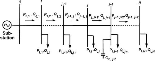
The sum of the losses in the line sections of the feeders, or the total power loss of the feeder, is given by (2) $$P^{\mathrm{T},\text{Loss}}=\sum _{j=0}^{N-1}\frac{P_{j,j+1}^2+Q_{j,j+1}^2}{{\left|V_j\right|}^2}{R}_{j,j+1}$$(2) where $R_{j,j+1}$ is the resistance of the line segment between the buses j and j + 1,$Q_{j,j+1},P_{j,j+1}$ are the reactive and real power flows between the buses j and j + 1, in kVAr and kW, V_j is the voltage at bus j.

2.1. Objective Function

The objective of the optimal capacitor location and sizing (OCLS) problem is to determine the optimal size and location of the capacitors to minimize the costs of capacitor investment, system power loss or energy loss. Hence the cost function that is to be minimized can be defined as [4, 6, 16] (3) $$\min F=\min \left(\text{total}\mathrm{ }\text{cost}\right)=K_P{P}^{T,\text{loss}}+\sum _{j=1}^n{K}_j^c{Q}_j^c+K_{\mathrm{e}}{E}_{\text{loss}}$$(3) where K_P is the equivalent annual cost per unit of power loss in $/(kW-year), j = 1,2,…, n are the indices of buses selected for compensation, $K_j^c$ is the annual cost per unit of reactive power injected at bus j in $/(kVAR-year), $Q_j^c$ is the capacitor size in kVAR, placed at bus j, K_e is the cost of energy loss per kWh, and E_loss is the energy loss in kWh.

2.2. Constraints

The inequality constraints of the problem are given by

1. The variation in the voltage at each bus should be well within the pre-defined permissible limits: (4) $$V_{j,\min }\le V_j\le V_{j,\max }$$(4)

2. Capacitors are commercially available only in discrete sizes. If there are L number of discrete sizes, the capacitor sizes belong to the set $\{Q_0^c,2Q_0^c,\dots ,L{Q}_0^c\},$ where $Q_0^c$ is the minimum size, and $L{Q}_0^c$ is the maximum size of the capacitors available.

3. The other constraints, which are nonlinear equality ones, are the set of power flow equations given by [4, 23,24] (Figure 1): (5) $$P_{j+1,j+2}=P_{j,j+1}-P_{j,j+1}^{\text{Loss}}-P_{\mathrm{L},j+1}$$(5) (6) $$Q_{j+1,j+2}=Q_{j,j+1}-Q_{j,j+1}^{\text{Loss}}-Q_{\mathrm{L},j+1}+Q_{\mathrm{c},j+1}$$(6) (7) $${\left|V_{j+1}\right|}^2={\left|V_j\right|}^2-2\left(R_{j,j+1}{P}_{j,j+1}+X_{j,j+1}{Q}_{j,j+1}\right)+\left(R_{j,j+1}^2+X_{j,j+1}^2\right)\left(\frac{P_{j,j+1}^2+Q_{j,j+1}^2}{{\left|V_j\right|}^2}\right)$$(7)

where $Q_{\mathrm{L},j+1}$ and $P_{\mathrm{L},j+1}$ are the reactive and real power loads at bus j + 1.

3. Grey Wolf Optimizer Algorithm

The GWO algorithm is a recently proposed optimization technique. It is considered as a population-based stochastic algorithm that estimates that global optimum of a given problem using a set of candidate solutions. This makes GWO able to avoid local solutions better than the conventional and gradient-based optimization algorithms. The main inspiration of GWO is the social interaction in a pack of grey wolves for hunting. As discussed in the seminal paper of this algorithm [29], grey wolves have a rigid social hierarchy that balances the power and leadership in the pack. Figure 2(a) illustrates different types of wolves and their leadership position in the pack.

Figure 2. Hierarchy of a pack of grey wolves [29].

To simulate the behavior of grey wolves, the following mathematical models have been proposed [29]: (8) $${\overrightarrow{X}}_1={\overrightarrow{X}}^{\alpha }-\mathrm{ }{\overrightarrow{A}}_1\otimes {\overrightarrow{D}}_{\alpha },{\overrightarrow{X}}_2={\overrightarrow{X}}^{\beta }-\mathrm{ }{\overrightarrow{A}}_2\otimes {\overrightarrow{D}}_{\beta },{\overrightarrow{X}}_3={\overrightarrow{X}}^{\delta }-\mathrm{ }{\overrightarrow{A}}_3\otimes {\overrightarrow{D}}_{\delta }$$(8) (9) $$\overrightarrow{X}\mathrm{(}t+1\mathrm{)}=\frac{{\overrightarrow{X}}_1+{\overrightarrow{X}}_2+{\overrightarrow{X}}_3}{3}$$(9) where ${\overrightarrow{X}}^{\alpha },$ ${\overrightarrow{X}}^{\beta }$ and ${\overrightarrow{X}}^{\delta }$ are the positions of the alpha, beta and delta wolves respectively, in the search space, $\overrightarrow{A}$ is a vector of values that impacts the movement, $\overrightarrow{D}$ is the distance, and $\otimes$ denotes to component-wise multiplication.

The parameters $\overrightarrow{A},$ $\overrightarrow{D},$ and $\overrightarrow{X}$ are calculated as follows: (10) $$\overrightarrow{D}=\left|\overrightarrow{C}\otimes {\overrightarrow{X}}^p\mathrm{(}t\mathrm{)}-\overrightarrow{X}\mathrm{(}t\mathrm{)}\right|$$(10) (11) $$\overrightarrow{C}=2{\overrightarrow{r}}_1$$(11) (12) $$\overrightarrow{X}\mathrm{(}t+1\mathrm{)}={\overrightarrow{X}}^p\mathrm{(}t\mathrm{)}-\mathrm{ }\overrightarrow{A}\otimes \overrightarrow{D}$$(12) (13) $$\overrightarrow{A}=a\mathrm{(}2{\overrightarrow{r}}_2-1\mathrm{)}$$(13) (14) $${\overrightarrow{D}}_{\alpha }=\left|{\overrightarrow{C}}_1\otimes {\overrightarrow{X}}^{\alpha }-\overrightarrow{X}\right|,{\overrightarrow{D}}_{\beta }=\left|{\overrightarrow{C}}_2\otimes {\overrightarrow{X}}^{\beta }-\overrightarrow{X}\right|{\overrightarrow{D}}_{\delta }=\left|{\overrightarrow{C}}_3\otimes {\overrightarrow{X}}^{\delta }-\overrightarrow{X}\right|$$(14) where $\overrightarrow{X}$ is the position of a wolf, t is the iteration counter, ${\overrightarrow{X}}^p$ is the position of prey, a decreases from 2 to 0 proportional to the number of iterations, ${\overrightarrow{r}}_1,$${\overrightarrow{r}}_2$ are vectors of random numbers extracted from a uniform distribution.

4. The Hybrid Grey Wolf Optimizer

The discrete values of the capacitor sizes and bus numbers make the OCP problem inherently discrete. Additionally, the nonlinear power balance equality constraint makes it non-convex. [30,31] introduced a hybrid GWO with evolutionary operators, to improve the search capability in such solution spaces that are non-convex. These are outlined below.

4.1. Crossover

The binomial or uniform crossover is used here. On applying crossover, the ith component of the jth wolf is given by (15) $$X_i^j=\mathrm{ }\{\begin{array}{l}{X}_{i\mathrm{ }}^r\mathit{\text{ if }}{\text{ rand}}_i^j<C_r\\ X_i^j \mathit{else}\end{array} i=1\text{ to }D,\mathrm{ }j=1\text{ to }{N}_w$$(15) where D is the size of the solution vector, N_w is the number of wolves or solutions, $r=1\text{to}{N}_w,r\ne j,$ chosen randomly, and ${\text{rand}}_i^j\in \left[0,1\right]$ is randomly generated ∀ i, j.

In this article, a dynamically varying value of the crossover probability $C_r$ was used. This is given by [32] (16) $$C_r=\frac{1}{5}\times {\widehat{F}}^{j,\text{best}}$$(16) (17) $${\widehat{F}}^{j,\text{best}}=\frac{F^j-F^{\text{best}}}{F^{\text{worst}}-F^{\text{best}}} j=1 \text{to} N_{\mathrm{w}}$$(17) where the worst and best values of fitness in the current generation or iteration of the wolf pack are identified as $F^{\text{worst}}$ and $F^{\text{best}}$ respectively, and $F^j$ is the fitness of the jth wolf. (16(16) $$C_r=\frac{1}{5}\times {\widehat{F}}^{j,\text{best}}$$(16) ) and (17(17) $${\widehat{F}}^{j,\text{best}}=\frac{F^j-F^{\text{best}}}{F^{\text{worst}}-F^{\text{best}}} j=1 \text{to} N_{\mathrm{w}}$$(17) ) ensure that the crossover rate or probability is directly proportional to the relative fitness of the vector and that the best wolf vector remains unchanged.

4.2. Mutation

Given some mutation rate or mutation probability µ, the ith component of the jth wolf after mutation is given by [30]: (18) $$x_i^j=\{\begin{array}{l}{x}^{\mathrm{gBest},\mathrm{ }i}+r_r(x_i^p-x_i^q) {\text{if rand}}_i^j<\mu \\ x_i^j \mathit{else}\end{array} i=1\mathrm{ }\text{to}D,j=1\mathrm{ }\text{to}\mathrm{ }{N}_w$$(18) (19) $$\mu =\frac{1}{20}\times {\widehat{F}}^{i,\text{best}}$$(19) where $p,q=1\text{to}{N}_w\text{are randomly}\mathrm{ }\text{generated},p\ne q\ne j,$ and $r_r, \text{and} {\text{rand}}_i^j\in \left[0,1\right]$ are also randomly generated ∀ i, j. $x^{{}_{\text{gBest},i}}$ is the ith component of the global best solution (or wolf), across the iterations, up to the current iteration. This global best wolf is compared with the best wolf in the pack of the current iteration. If the global best wolf is better than the best wolf, it continues to be the global best wolf. Else, it is replaced by the best wolf. Equations (17)(17) $${\widehat{F}}^{j,\text{best}}=\frac{F^j-F^{\text{best}}}{F^{\text{worst}}-F^{\text{best}}} j=1 \text{to} N_{\mathrm{w}}$$(17) and (19)(19) $$\mu =\frac{1}{20}\times {\widehat{F}}^{i,\text{best}}$$(19) mean that the mutation rate or mutation probability µ is 1/20 for the worst wolf and 0 for the best wolf of the current generation.

5. HGWO Implementation for the OCP Problem

The losses can be reduced and the voltage profile improved by placement of capacitors at appropriate locations. The locations and sizes of the capacitors are the control variables of the problem. A wolf or solution vector comprises these two types of control variables. Load flow study based on [33] is executed for each solution, to find the bus voltages and system losses. The fitness of each solution is the loss obtained.

The stepwise procedure for solving the OCP optimization problem using HGWO is as follows:

• Step 0: The population size N_w, number of iterations, number of locations for capacitors to be installed nc, size of capacitors Q in kVAR are chosen.

N_w number of feasible solution vectors, or wolves, satisfying the constraints in Section 2.2. are generated. These form the initial population [9] (20) $$\mathit{P}=\left[\begin{array}{c}{P}^1\\ P^2\\ ⋮\\ P^{N_w}\end{array}\right]=\left[\begin{array}{cccccccc}{l}_1^1& l_2^1& \cdots & l_n^1& Q_1^{c1}& Q_2^{c1}& \cdots & Q_n^{c1}\\ l_1^1& l_2^2& \cdots & l_n^2& Q_1^{c2}& Q_2^{c2}& \cdots & Q_n^{c2}\\ ⋮& \cdots & & & ⋮& \dots & & ⋮\\ l_1^{N_w}& l_2^{N_w}& \cdots & l_n^{N_w}& Q_1^{c{N}_w}& Q_2^{c{N}_w}& \cdots & Q_n^{c{N}_w}\end{array}\right]$$(20) where j = 1 to n is the bus number or location, $Q_j^{c1}$ is the capacitor size at location l, in kVAR.

• Step 1: The power loss in the distribution system for each wolf is determined by running the load flow for each wolf. The fitness of each wolf is evaluated using the objective or fitness function (3). The global best solution P^gBest, and the α, β and δ wolves are identified. P^gBest = P^α, in the very first iteration.

• Step 2: ${\overrightarrow{D}}_{\alpha },{\overrightarrow{D}}_{\beta }\text{and}{\overrightarrow{D}}_{\delta }$ are computed by applying the encircling operator (10):

(21) $${\overrightarrow{D}}_{\alpha }=\left|{\overrightarrow{C}}_1\otimes {\overrightarrow{P}}^{\alpha }-{\overrightarrow{P}}^j\right|,{\overrightarrow{D}}_{\beta }=\left|{\overrightarrow{C}}_2\otimes {\overrightarrow{P}}^{{}_{\beta }}-{\overrightarrow{P}}^j\right|,{\overrightarrow{D}}_{\delta }=\left|{\overrightarrow{C}}_3\otimes {\overrightarrow{P}}^{{}_{\delta }}-{\overrightarrow{P}}^j\right|$$(21)

$\overrightarrow{P_1},$ $\overrightarrow{P_2}$ and $\overrightarrow{P_3}$ are computed by applying the hunting operator (12). First the distances are calculated using (21). Using these distances, (22) $${\overrightarrow{P}}_1={\overrightarrow{P}}^{\alpha }-\mathrm{ }{\overrightarrow{A}}_1\otimes {\overrightarrow{D}}_{\alpha },{\overrightarrow{P}}_2={\overrightarrow{P}}^{\beta }-\mathrm{ }{\overrightarrow{A}}_2\otimes {\overrightarrow{D}}_{\beta },{\overrightarrow{P}}_3={\overrightarrow{P}}^{\delta }-\mathrm{ }{\overrightarrow{A}}_1\otimes {\overrightarrow{D}}_{\delta }$$(22) The next generation population, $\mathit{P}\mathrm{(}t+1\mathrm{)},$ consisting of N_w number of wolves or solutions is computed next. The individual wolf of the population is calculated as (23) $${\overrightarrow{P}}^i\mathrm{(}t+1\mathrm{)}=\frac{{\overrightarrow{P}}_1+{\overrightarrow{P}}_2+{\overrightarrow{P}}_3}{3}$$(23)

• Step 3: The operators of crossover (15) and mutation (18) are applied, with $P_i^j$ replacing $X_i^j.$

• Step 4: The components of the new solution are rounded off to their nearest discrete values, given in Table 1.

• Step 5: Check if the termination criterion is satisfied. Stop, if yes. If not, repeat steps 1 to 4.

TABLE 1. Assumed capacitor sizes and cost/(kVAR-year).

j	1	2	3	4	5
Capacitor size, Qc (kVAR)	150	300	450	600	750
Cost ($/kVAR-year)	0.500	0.350	0.253	0.220	0.276
j	6	7	8	9	10
Capacitor size, Qc (kVAR)	900	1050	1200	1350	1500
Cost ($/kVAR-year)	0.183	0.228	0.170	0.207	0.201

6. Test Cases, Results and Discussion

The proposed HGWO approach is applied to four test cases comprising IEEE 34-, 69-, 119-bus RDSs, and a practical 22-bus RDS. The size of the population or pack or trial solutions is fixed at 40. The maximum number of iterations iter_max is used as the stopping criterion. iter_max is increased as the size of the problem increases. Accordingly, iter_max is 200 for 22- and 34-bus RDSs, and 250 for 69-bus RDS and 400 for 119-bus RDS. The bus voltage limits are taken as V_min=0.9 p.u. and V_max=1.1 p.u. [4, 17,18, 21]. Table 1 shows the sizes of the capacitors that are limited to discrete values, and their associated costs, for the first three test cases. The cost of real power loss assumed to be 168 $/(kW-year) as in [20], and the energy loss component given by $K_{\mathrm{e}}{E}_{\text{loss}}$ in (3) is not considered for the first three cases. The simulation is carried out using MATLAB® software. The personal computer used was of 3 GHz, 64 bit, with i7 processor and 6 GB RAM. The results obtained on these cases are compared with those reported in the literature. Also included in this article are the statistical analysis of the results obtained by using the HGWO method of this article. The best, worst, mean total cost and the standard deviation for each of the test cases over fifty independent trial runs are part of the results.

6.1 34-Bus RDS

The one-line diagram of the 34-bus RDS is shown in Figure 3 [20]. The system has 33 distribution lines and 34 buses, and a total reactive and real power demand of 2,873.5 kVAR and 4,636.5 kW, respectively.

Figure 3. One-line diagram of the 34-bus RDS.

The real power loss and minimum voltage for the uncompensated case—determined by running the load flow—are 221.73 kW and 0.9416 p.u., respectively. To show the validity and effectiveness of the proposed HGWO method, the results obtained are compared against those obtained by other recent methods in the literature (Table 2). The HGWO method yields a power loss of 160.47 kW, the least of all methods with the exception of SAMHBMO. Increasing the number of capacitor locations beyond three can further reduce the losses, for the same total kVAR, which is the case in SAMHBMO. (i) MINLP method [6] reports a power loss of 157.53 kW with six capacitor locations, capacitor sizes in multiples of hundred kVAR, and a total installed capacitance of 2,800 kVAR. The HGWO method with six capacitor locations (at buses 6, 4, 25, 8, 21 and 11) and capacitor sizes in multiples of one hundred and fifty (450, 450, 600, 300, 600, 450 kVAR, total = 2,850 kVAR) yields a power loss of 158.51 kW (not a part of Table 2), and (ii) Fuzzy based approach [20] gives a power loss of 162 kW, for nine locations, for a total installed capacity of 3,450 kVAR. The HGWO method with nine locations gives a loss of 158.57 kW for the locations 10, 5, 12, 25, 6, 8, 3, 2 and 21, for capacitor values of 150, 300, 150, 600, 450, 450, 150, 300 and 600 kVAR respectively, a total of 3,150 kVAR. These comparisons show the better performance of HGWO with other methods. The table also shows the comparisons of total kVAR of the installed capacitor sizes, costs of the capacitors, cost of kW loss, total cost, net savings, and percentage savings. This savings is highest of all for the HGWO, with the exception of SAMHBMO. Also included are the statistical analysis of the results by using the HGWO method of this article. The best, worst, mean total cost and the standard deviation for each of the test cases over fifty independent trial runs are part of the results. It may be noted that such an analysis is a first for this test case, since none of the other results has this analysis for this test case.

TABLE 2. Simulation results and comparison for the 34-bus RDS.

Description	Base Case	GA [34]	ACO [9]	ET [35]	MMS [26]	SAMHBMO [36]	HGWO
Total loss(kW)	221.73	164.96	164.508	161.33	160.92	159.709	160.47
Vmin (p.u)	0.9416	0.9478	0.9501	0.9506	0.9506	0.9501	0.9505
CLocation (Bus no.)	–	5, 9, 12, 22, 26	9, 19, 25	8, 18, 25	8, 12, 18, 21, 24, 25, 28	9, 16, 20, 23	8, 18, 23
CSize (kVAR)	–	300, 300, 300, 600, 300	450, 450, 1050	1050, 750, 750	150, 450, 450, 600, 150, 450, 300	600, 600, 600, 600	750, 900, 750
Total kVAR	–	1,800	1,950	2,550	2,550	2,400	2,400
Cost of capacitor ($/(kVAR-year))		552.00	467.1	653.54	728.55	528	578.7
Cost of kW loss ($/year)	37,250.64	27,713.28	27,637.344	27,103.44	27,034.56	26,831.11	26,958.96
Total cost		28,265.28	28,104.44	27,756.84	27,763.11	27,359.11	27,537.66
Net savings ($/year)		8,985.36	9,146.20	9,493.8	9,487.53	9,890.43	9,712.98
Savings (%)		24.12	24.55	25.49	25.47	26.55	26.08
Worst cost ($/year)	--	NA	NA	NA	NA	NA	27,603.00
Best cost ($/year)	--	NA	NA	NA	NA	NA	27,537.66
Mean cost ($/year)	--	NA	NA	NA	NA	NA	27,538.50
Std. deviation	--	NA	NA	NA	NA	NA	30.1568

NA = not available.

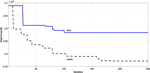
Figure 4 shows the voltage profile of the 34-bus RDS without and with capacitor compensation. A good improvement in the voltage profile may be noted at the buses where the voltages are very low without capacitors. The convergence curves of minimum fitness values of the GWO and HGWO for the 34-bus RDS is shown in Figure 5. The improved performance of the HGWO over the GWO is clearly noticeable.

Figure 4. Voltage profile of the 34-bus RDS without and with capacitor compensation.

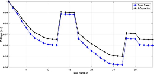
Figure 5. Typical convergence curves of the GWO and HGWO for the 34-bus RDS.

6.2 69-Bus RDS

The one-line diagram of the 69-bus system is shown in Figure 6 [37]. It has 68 distribution lines and 69 buses. The rated load of the system is 3,801.4 kW and 2,693.6 kVAR [37]. The real power loss and minimum voltage for the uncompensated case—determined from the load flow—are 225 kW and 0.9092 p.u., respectively. The validity and effectiveness of the proposed HGWO method is tested by comparison of the results produced against the other recently reported results. The optimal capacitor sizes and locations obtained by using the HGWO method and those obtained by other methods are shown in Table 3. It is observed from the table that, the HGWO method gives a power loss of 145.22 kW, which is the least of all values reported, and equals the value by inclusion and interchange of variables (IIV) method, and a minimum voltage of 0.9308 p.u. The table also shows the comparisons of the total kVAR of the capacitor sizes installed, cost of kW loss, total cost, net savings and percentage savings. Also included are the statistical analysis of the results by using the HGWO method of this article. The best, worst, mean total cost and the standard deviation for each of the test cases over fifty independent trial runs are part of the results. It may be noted that such analyses are either not available, or not applicable for comparison with the analysis in this article.

Figure 6. One-line diagram of the 69-bus RDS.

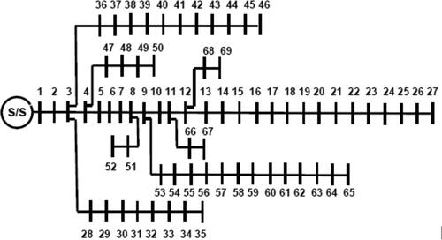
TABLE 3. Simulation results and comparison for the 69-bus RDS.

Description	Base Case	Heuristic method [17]	DSA [18]	TLBO [21]	GSA [11]	IIV [27]	HGWO
Total loss (kW)	225	148.48	147.00	146.35	145.9	145.22	145.22
Vmin (p.u)	0.9092	0.9305	0.9317	0.9313	0.9511	0.9308	0.9308
CLocation (Bus no.)	–	8, 58, 60	61, 15, 60	12, 61, 64	26,13,15	11, 17, 61	11, 17, 61
CSize (kVAR)	–	600, 150, 1050	900, 450, 450	600, 1050,150	150, 150, 1050	300, 300, 1200	300,300,1200
Total kVAR	–	1800	1800	1800	1350	1800	1800
Cost of capacitor ($/(kVAR-year))	–	446.4	392.4	446.4	389.4	414	414
Cost of kW loss ($/year)	37,800	24,944.64	24,696	24,586.8	24,511.20	24,396.96	24,396.96
Total cost		25,391.04	25,088.4	25,033.2	24,900.6	24,810.96	24,810.96
Net savings ($/year)		12,408.96	12,711.6	12,766.8	12,899.4	12,989.04	12,989.04
Savings (%)		32.83	33.63	33.77	34.13	34.36	34.36
Worst cost ($/year)	--	NA	NA	NA**	NA	NA	25,253.00
Best cost ($/year)	--	NA	NA	NA**	NA	NA	24,810.96
Mean cost ($/year)	--	NA	NA	NA**	NA	NA	25,014.0
Std. deviation	--	NA	NA	NA**	NA	NA	121.611

NA = not available. NA**= not applicable.

Figure 7 shows the voltage profile improvement of the 69-bus system after the addition of capacitors for compensation. The convergence curves of minimum fitness values of the HGWO and GWO for the 69-bus RDS is also shown in Figure 8. The improved performance of the HGWO over the GWO is clearly noticeable.

Figure 7. Voltage profile of the 69-bus RDS without and with capacitor compensation.

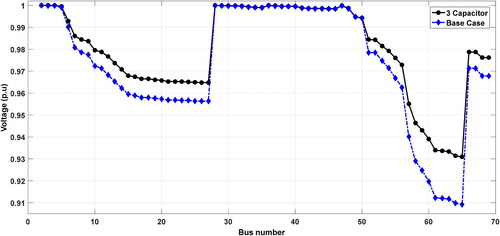
Figure 8. Typical convergence curves of the GWO and HGWO for the 69-bus RDS.

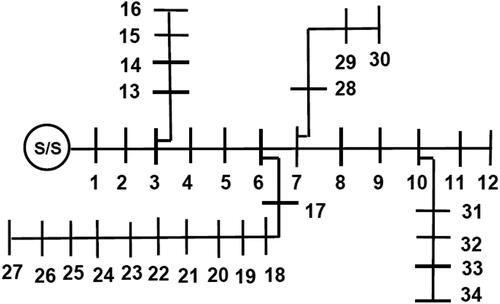
6.3 119-Bus RDS

The one-line diagram of the 119-bus system is shown in Figure 9. This test system comprises 119 buses and 117 lines. The total kVA demand of this system is 22,709.72 kW and 17,041.07 kVAR. The base values are 11 kV and 100 MVA. The line data and load are given in [38]. The uncompensated case gives a real power loss and minimum voltage of 1294.35 kW and 0.8688 p.u., respectively. The optimal capacitor sizes and locations obtained by using the HGWO method and the other methods are shown in Table 4. It is observed from the table that, the HGWO method gives a power loss of 836.97 kW, which is the least of all values reported, and a minimum voltage of 0.9089 p.u. The reduction in power loss is substantial, at 6 kW. Since the capacitor sizes in the other references are assumed to be either continuous, or discrete multiples of other sizes, the cost of capacitors are not considered for comparison. The table also compares the total kVAR of the capacitor sizes installed, cost of kW loss, total cost, net savings and percentage savings. The statistical analysis is also shown.

Figure 9. One-line diagram of the 119-bus RDS.

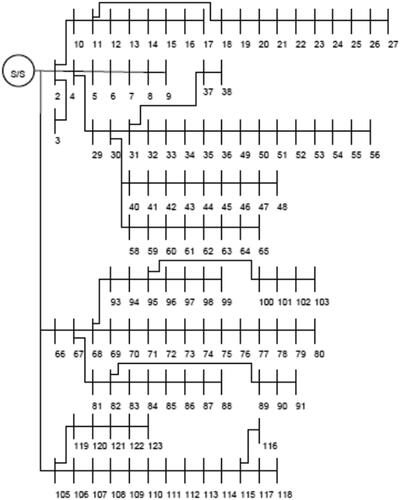
TABLE 4. Simulation results and comparison for the 119-bus RDS.

Description	Base Case	HSA-PABC [11]	Heuristic Approach [34]	ABC [7]	FPA [15]	Improved Harmony Search [25]	HGWO
Total loss (kW)	1,294.35	856.96	854.42	853.39	844.47	843.146	836.97
Vmin (p.u)	0.8688	0.9132	0.9107	0.9088	0.9002	0.9020	0.9089
CLocation (Bus no.)		99, 111, 111, 111, 86, 76, 108, 49, 71, 50	C at 15 locations	32, 35, 40, 50, 70, 73, 79, 105, 106, 109, 110	39, 43, 70, 74, 86, 91, 107, 109, 118	39,43,70, 74, 86, 91,107, 109,118	41,49,51,59,73, 78,96,106,110
CSize (kVAR)		1000, 1300, 1500, 550, 1350, 1450, 1350, 1500	9750 at 15 locations	850,1050,1300, 800, 550, 1300,1200,700 250,800,1200	1500, 600, 500, 1050, 900, 1500, 700, 500,1050	1500,1000, 1000, 1000, 900,1500 850,850,1200	1050,900,1050,1050, 1500,1500,1200, 1500, 1350
Total kVAR		10,000	9,750	10,000	8,300	9,800	11,100
Cost of capacitor ($/(kVAR-year))		NA	NA	NA	NA	NA	2,270.85
Cost of kW loss ($/year)	217,450.8	143,969.28	143,374.56	143,369.52	141,870.96	141,648.53	140,610.96
Total cost		NA	NA	NA	NA	NA	142,881.81
Net savings ($/year)		NA	NA	NA	NA	NA	74,568.99
Savings (%)		NA	NA	NA	NA	NA	34.29
Worst cost ($/year)	--	NA	NA	NA	NA	NA	151,014.96
Best cost ($/year)		NA	NA	NA	NA	NA	142,881.81
Mean cost ($/year)	--	NA	NA	NA	NA	NA	147,703.68
Std. deviation	--	NA	NA	NA	NA	NA	1,791.75

NA = not applicable

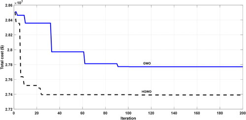
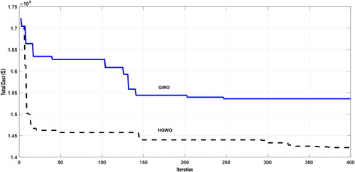
Figure 10 shows the voltage profile improvement of the 119-bus system after the addition of capacitor compensation. The convergence curves of minimum fitness values of the HGWO and GWO for the 119-bus RDS is also shown in Figure 11. The improved performance of the HGWO over the GWO is clearly noticeable.

Figure 10. Voltage profile of the 119-bus RDS without and with capacitor compensation.

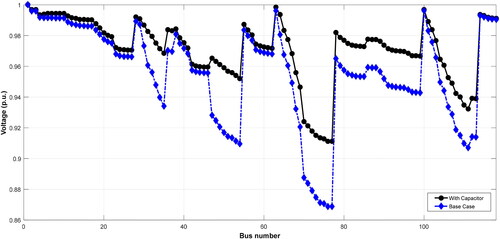
Figure 11. Sample convergence curves of the HGWO and GWO for the 119-bus RDS.

6.4. 22-Bus Practical RDS

Since the load on a distribution system is not constant and varies through the year, the OCP problem has to be studied for different load levels. Hence a practical, 22-bus RDS from Eastern part of India is considered. This test system comprises 22 buses and 21 lines [18]. For this case, the energy loss component given by $K_{\mathrm{e}}{E}_{\text{loss}}$ in (3) is considered, and the power loss component given by $K_P{P}^{T,\text{loss}}$ is not considered, unlike for the first three cases. The load variation is grouped under three different levels. These levels and their durations are: light load of 50% for a duration of 2000 hours, nominal load of 100% for 5,260 hours, and peak load of 160% for 1500 hours. The objective is to minimize the total cost of energy loss and the cost of the capacitors. The base voltage is 11 kV, real and reactive power loads are 662.311 kW and 657.4 kVAR, respectively. The base case power loss for these three load levels are 4.31 kW, 17.67 kW and 46.59 kW respectively. The cost of energy is assumed as 0.06 USD/kWh, and the cost of capacitor as 3.0 USD/kVAR.

Table 5 shows the results obtained by using the HGWO method for the power loss, minimum bus voltages, capacitor locations, and their sizes for the three levels of peak, nominal and light loads. Also shown are the total optimal kVAR, cost of capacitor, and cost of energy loss obtained by using the HGWO. The results by other methods are also shown. The total cost by the HGWO method is the least of all with the exception of that by the CBO.

TABLE 5. Simulation results and comparison for the 22-bus practical RDS.

Description	DSA [18]	CBO [39]	TLBO [21]	HGWO
Total Loss(kW) Ppeak / Pnom. / Plight	24.89 / 9.66 / 2.39	32.93 / 9.78 / 2.59	24.43 / 9.31 / 2.39	24.19 / 9.37 / 2.37
Vmin (p.u)	0.9701 / 0.9824 / 0.9909	0.9621 / 0.9816 / 0.9924	0.9712 / 0.9822 / 0.9903	0.9702 / 0.9811 / 0.9915
CLocation(Bus no.) CSize(kVAR) Cpeak / Cnom. / Clight	4 150 / 150 / 0 13 450 / 300 / 150 16 300 / 150 / 150 17 150 / 150 / 0	18 150 / 300 / 150 20 150 / 150 / 150	9 150 / 150 / 150 14 300 / 150 / 0 17 150 / 150 / 150 20 300 / 150 / 0	5 150 / 150 / 0 12 150 / 150 / 150 15 300 / 150 / 0 19 300 / 150 / 150
Total optimal kVAR	1050	450	900	900
Cost of capacitor ($)	3150	1350	2700	2700
Cost of energy loss ($)	5575.59	6360.82	5423.33	5418.67
Best total cost ($)	8725.59	7710.82	8123.33	8118.67
Worst total cost ($)	--	--	8158.51	8187.37
Mean total cost ($)	--	--	8134.65	8138.17
Std. deviation	--	--	0.02058	0.1075

7. Conclusion

A new metaheuristic algorithm, the HGWO, was used to solve the OCPS, a discrete, non-convex optimization problem. Examples considered are the IEEE 34-, 69-, 119-bus RDSs and the 22-bus practical RDS. In terms of optimality, the results compare well with the other best results in the literature. This suggests that the results obtained may be the global optima for the given problems and choices made.

Further improvement in the results is possible if the number of capacitor locations are increased, and capacitances are treated as continuously variable, as has been done in some references. However, the number of capacitor locations in this work were chosen to enable fair comparison with other reported results. A similar comment can be made about the choice of capacitor sizes.

Convex programming problems (CPPs) are best solved by gradient based, or classical methods. Problems like the optimal capacitor placement problem that are not CPPs are more easily solved by metaheuristic methods, since these are free from the requirement of convexity conditions. However, this capability is not always a given; it is very much algorithm dependent. This article shows that, the HGWO has the operators to search the solution space thoroughly.

Application of the HGWO algorithm to other intractable optimization problems in the area of power systems and other fields can be considered for future work

Acknowledgment

The first two authors thank VIT for providing “VIT SEED GRANT” for carrying out this research work.

Additional information

Notes on contributors

T. Jayabarathi

T. Jayabarathi obtained her bachelor’s degree in electrical engineering from Dharwar University, Dharwar, India, in 1985, Master’s degree in power systems from Annamalai University, India, and Ph.D. from College of Engineering, Guindy, Anna University, Chennai, India, in 2000. Currently, she is Professor (Higher Academic Grade), School of Electrical Engineering, Vellore Institute of Technology, Vellore, India. Her current research interests are in optimization, soft computing, and optimization in power systems.

T. Raghunathan

T. Raghunathan obtained his bachelor’s degree in electrical engineering from Bangalore University, Bangalore, India, in 1989, and Master’s degree in Control and Instrumentation Engineering from College of Engineering, Guindy, Anna University, Chennai, India, in 2000, and PhD from Indian Institute of Science, Bangalore, India, in 2012. Currently, he is Professor (Higher Academic Grade), School of Electrical Engineering, Vellore Institute of Technology, Vellore, India. He served as engineer with Coal India Limited, a public sector undertaking of the Government of India, from Dec. 1991 to Oct. 2000. From Aug. 1996, he was Executive Engineer (E&M), until Oct. 2000. From March 2002 to July 2004, he was Senior Lecturer with the electrical engineering dept., Vellore Institute of Technology, Vellore, India. His current research interests are in engineering optimization, soft computing, optimal control and optimization in power systems.

R. Sanjay

R. Sanjay received his bachelor’s degree in electrical and electronics engineering from Vellore Institute of Technology, India, in 2017. He is currently pursuing the Ph.D. degree with the Semiconductor Power Electronics Center (SPEC) at The University of Texas at Austin, TX, USA. His current research interests include solid state transformers, medium voltage AC/DC and AC/AC converters and renewable energy integrations.

Aditya Jha

Aditya Jha received B.Tech. degree in electrical and electronics engineering from Vellore Institute of Technology, Vellore, India, in 2018 and M. Tech. degree in power electronics & power systems from IIT Bombay in 2021. From 2021 started working in Systems & Control Engineering at Eaton eMobility, Pune. His areas of interest include microgrids, electric drives, and optimization algorithms for power systems.

S. Mirjalili

Seyedali Mirjalili is Professor and the founding director of Centre for Artificial Intelligence Research and Optimization, Torrens University Australia, and Adjunct Professor with Griffith University, Australia. He is an Associate Editor of several AI journals, including Neurocomputing, Applied Soft Computing, Advances in Engineering Software, Computers in Biology and Medicine, Healthcare Analytics, and Applied Intelligence. His interests are in optimization algorithms and machine learning.

S. Hari Charan Cherukuri

S. Hari Charan Cherukuri received his B.E. degree in electrical and electronics engineering from Anna University, Chennai, India, in 2011, M.Tech. degree in power systems from SASTRA University, Thanjavur, India, in 2014, and PhD degree from the Vellore Institute of Technology (VIT), Vellore, India in 2019. After completion of his PhD, he was with the Power Systems and Smart Grid Laboratory, Discipline of Electrical Engineering, IIT Gandhinagar as a Research Associate until July 2021. Currently he is working in Marelli India Pvt. Ltd. as a Deputy Manager – R & D in the electric power train division. His research interests include energy management in grid interactive micro grids, electric springs and demand side management, home energy management, and application of optimization techniques to power system problems.

References

- M. M. Aman, G. B. Jasmon, A. H. A. Bakar, H. Mokhlis and M. Karimi, “Optimum shunt capacitor placement in distribution system—a review and comparative study,” Renew. Sustain. Energy Rev., vol. 30, pp. 429–439, 2014. DOI: 10.1016/j.rser.2013.10.002.
- H. Dura, “Optimum number, location, and size of shunt capacitors in radial distribution feeders a dynamic programming approach,” IEEE Trans. Power App. Syst., vol. PAS-87, no. 9, pp. 1769–1774, 1968. DOI: 10.1109/TPAS.1968.291982.
- J. H. Grainger and S. H. Lee, “Optimum size and location of shunt capacitors for reduction of losses on distribution feeders,” IEEE Trans. Power App. Syst., vol. PAS-100, no. 3, pp. 1105–1118, 1981. DOI: 10.1109/TPAS.1981.316577.
- M. E. Baran and F. F. Wu, “Optimal sizing of capacitors placed on a radial distribution system,” IEEE Trans. Power Delivery, vol. 4, no. 1, pp. 735–743, 1989. DOI: 10.1109/61.19266.
- H. M. Khodr, F. G. Olsina, P. M. De Oliveira-De Jesus and J. M. Yusta, “Maximum savings approach for location and sizing of capacitors in distribution systems,” Electric Power Syst. Res., vol. 78, no. 7, pp. 1192–1203, 2008. DOI: 10.1016/j.epsr.2007.10.002.
- S. Nojavan, M. Jalali and K. Zare, “Optimal allocation of capacitors in radial/mesh distribution systems using mixed integer nonlinear programming approach,” Electric Power Syst. Res., vol. 107, pp. 119–124, 2014. DOI: 10.1016/j.epsr.2013.09.019.
- A. A. El-Fergany and A. Y. Abdelaziz, “Artificial bee colony algorithm to allocate fixed and switched static shunt capacitors in radial distribution networks,” Electric Power Component. Syst., vol. 42, no. 5, pp. 427–438, 2014. DOI: 10.1080/15325008.2013.856965.
- A. R. Abul’Wafa, “Optimal capacitor placement for enhancing voltage stability in distribution systems using analytical algorithm and fuzzy-real coded GA,” Int. J. Elect. Power Energy Syst., vol. 55, pp. 246–252, 2014. DOI: 10.1016/j.ijepes.2013.09.014.
- A. A. El-Ela, R. A. El-Sehiemy, A. M. Kinawy and M. T. Mouwafi, “Optimal capacitor placement in distribution systems for power loss reduction and voltage profile improvement,” IET Generat. Trans. Distribut., vol. 10, no. 5, pp. 1209–1221, 2016. DOI: 10.1049/iet-gtd.2015.0799.
- K. Muthukumar and S. Jayalalitha, “Multiobjective hybrid evolutionary approach for optimal planning of shunt capacitors in radial distribution systems with load models,” Ain Shams Eng. J., vol. 9, no. 4, pp. 1975–1988, 2018. DOI: http://doi.org/10.1016/j.asej.2017.02.002.
- Y. M. Shuaib, M. S. Kalavathi and C. C. A. Rajan, “Optimal capacitor placement in radial distribution system using gravitational search algorithm,” Int. J. Elect. Power Energy Syst., vol. 64, pp. 384–397, 2015.
- K. R. Devabalaji, K. Ravi and D. P. Kothari, “Optimal location and sizing of capacitor placement in radial distribution system using Bacterial Foraging Optimization Algorithm,” Int. J. Elect. Power Energy Syst., vol. 71, pp. 383–390, 2015. DOI: 10.1016/j.ijepes.2015.03.008.
- M. A. Imran and M. Kowsalya, “Optimal distributed generation and capacitor placement in power distribution networks for power loss minimization,” Advances in Electrical Engineering (ICAEE), 2014 International Conference on, 2014. IEEE.
- A. Elsheikh, Y. Helmy, Y. Abouelseoud and A. Elsherif, “Optimal capacitor placement and sizing in radial electric power systems,” Alexandria Eng. J., vol. 53, no. 4, pp. 809–816, 2014. DOI: 10.1016/j.aej.2014.09.012.
- A. Y. Abdelaziz, E. S. Ali and S. M. Abd Elazim, “Optimal sizing and locations of capacitors in radial distribution systems via flower pollination optimization algorithm and power loss index,” Eng. Sci. Technol. Int. J., vol. 19, no. 1, pp. 610–618, 2016. DOI: 10.1016/j.jestch.2015.09.002.
- A. Y. Abdelaziz, E. S. Ali and S. M. Abd Elazim, “Flower pollination algorithm and loss sensitivity factors for optimal sizing and placement of capacitors in radial distribution systems,” Int. J. Electric Power Energy Syst., vol. 78, pp. 207–214, 2016. DOI: 10.1016/j.ijepes.2015.11.059.
- A. Hamouda, N. Lakehal and K. Zehar, “Heuristic method for reactive energy management in distribution feeders,” Energy Convers. Manage., vol. 51, no. 3, pp. 518–523, 2010. DOI: 10.1016/j.enconman.2009.10.016.
- Raju, M. Ramalinga, K. V. S. Ramachandra Murthy and K. Ravindra, “Direct search algorithm for capacitive compensation in radial distribution systems,” Int. J. Elect. Power Energy Syst., vol. 42, no. 1, pp. 24–30, 2012. DOI: 10.1016/j.ijepes.2012.03.006.
- S. K. Injeti, V. K. Thunuguntla and M. Shareef, “Optimal allocation of capacitor banks in radial distribution systems for minimization of real power loss and maximization of network savings using bio-inspired optimization algorithms,” Int. J. Elect. Power Energy Syst., vol. 69, pp. 441–455, 2015. DOI: 10.1016/j.ijepes.2015.01.040.
- H. A. Ramadan, M. A. Wahab, A. H. M. El-Sayed and M. M. Hamada, “A fuzzy-based approach for optimal allocation and sizing of capacitor banks,” Electric Power Syst. Res., vol. 106, pp. 232–240, 2014. DOI: 10.1016/j.epsr.2013.08.019.
- S. Sultana and P. K. Roy, “Optimal capacitor placement in radial distribution systems using teaching learning based optimization,” Int. J. Elect. Power Energy Syst., vol. 54, pp. 387–398, 2014. DOI: 10.1016/j.ijepes.2013.07.011.
- A. El-Fergany and A. Y. Abdelaziz, “Capacitor allocations in radial distribution networks using cuckoo search algorithm,” IET Generat. Trans. Distribut., vol. 8, no. 2, pp. 223–232, 2014. DOI: 10.1049/iet-gtd.2013.0290.
- C. S. Lee, H. V. H. Ayala and L. d Santos Coelho, “Capacitor placement of distribution systems using particle swarm optimization approaches,” Int. J. Elect. Power Energy Syst., vol. 64, pp. 839–851, 2015. DOI: 10.1016/j.ijepes.2014.07.069.
- J. P. Chiou and C. F. Chang, “Development of a novel algorithm for optimal capacitor placement in distribution systems,” Int. J. Elect. Power Energy Syst., vol. 73, pp. 684–690, 2015. DOI: 10.1016/j.ijepes.2015.06.003.
- E. S. Ali, S. A. Elazim and A. Y. Abdelaziz, “Improved Harmony Algorithm for optimal locations and sizing of capacitors in radial distribution systems,” Int. J. Elect. Power Energy Syst., vol. 79, pp. 275–284, 2016. DOI: 10.1016/j.ijepes.2016.01.015.
- F. G. Duque, L. W. de Oliveira, E. J. de Oliveira, A. L. Marcato and I. C. Silva, “Allocation of capacitor banks in distribution systems through a modified monkey search optimization technique,” Int. J. Elect. Power Energy Syst., vol. 73, pp. 420–432, 2015. DOI: 10.1016/j.ijepes.2015.05.034.
- I. P. Abril, “Algorithm of inclusion and interchange of variables for capacitors placement,” Electric Power Syst. Res., vol. 148, pp. 117–126, 2017.
- A. Khodabakhshian and M. H. Andishgar, “Simultaneous placement and sizing of DGs and shunt capacitors in distribution systems by using IMDE algorithm,” Int. J. Elect. Power Energy Syst., vol. 82, pp. 599–607, 2016. DOI: 10.1016/j.ijepes.2016.04.002.
- S. Mirjalili, S. M. Mirjalili and A. Lewis, “Grey wolf optimizer,” Adv. Eng. Softw., vol. 69, pp. 46–61, Mar2014. DOI: 10.1016/j.advengsoft.2013.12.007.
- T. Jayabarathi, T. Raghunathan, B. R. Adarsh and P. N. Suganthan, “Economic dispatch using hybrid grey wolf optimizer,” Energy, vol. 111, pp. 630–641, 2016. DOI: 10.1016/j.energy.2016.05.105.
- R. Sanjay, T. Jayabarathi, T. Raghunathan, V. Ramesh and N. Mithulananthan, “Optimal allocation of distributed generation using hybrid grey wolf optimizer,” IEEE Access, vol. 5, pp. 14807–14818, 2017. DOI: 10.1109/ACCESS.2017.2726586.
- A. H. Gandomi, A. H. and Alavi, Dec, “Krill herd: a new bio-inspired optimization algorithm,” Commun. Nonlinear Sci. Numer. Simul., vol. 17, no. 12, pp. 4831–4845, 2012. DOI: 10.1016/j.cnsns.2012.05.010.
- J.-H. Teng, “A direct approach for distribution system load flow solutions,” IEEE Trans. Power Delivery., vol. 18, no. 3, pp. 882–887, 2003.
- A. A. El-Fergany and A. Y. Abdelaziz, “Efficient heuristic-based approach for multi-objective capacitor allocation in radial distribution networks,” IET Generat. Trans. Distribut., vol. 8, no. 1, pp. 70–80, 2014. DOI: 10.1049/iet-gtd.2013.0213.
- A. Elmaouhab, M. Boudour and R. Gueddouche, “New evolutionary technique for optimization shunt capacitors in distribution networks,” J. Elect. Eng., vol. 62, no. 3, pp. 163–167, 2011. DOI: 10.2478/v10187-011-0027-x.
- A. Kavousi-Fard and T. Niknam, “Considering uncertainty in the multi-objective stochastic capacitor allocation problem using a novel self adaptive modification approach,” Electric Power Syst. Res., vol. 103, pp. 16–27, 2013. DOI: 10.1016/j.epsr.2013.04.010.
- J. S. Savier and D. Das, “Impact of network reconfiguration on loss allocation of radial distribution systems,” IEEE Trans. Power Delivery, vol. 22, no. 4, pp. 2473–2480, 2007. DOI: 10.1109/TPWRD.2007.905370.
- D. Zhang, Z. Fu and L. Zhang, “An improved TS algorithm for loss-minimum reconfiguration in large-scale distribution systems,” Electric Power Syst. Res., vol. 77, no. 5-6, pp. 685–694, 2007. DOI: 10.1016/j.epsr.2006.06.005.
- J. Vuletić and M. Todorovski, “Optimal capacitor placement in radial distribution systems using clustering based optimization,” Int. J. Elect. Power Energy Syst., vol. 62, pp. 229–236, 2014. DOI: 10.1016/j.ijepes.2014.05.001.