A mathematical model for cell cycle control: graded response or quantized response

ABSTRACT

Cell cycle is an important and complex biological system. A lot of efforts have been put in understanding cell cycle arrest for its vital role in clinical therapies. The cell-cycle-arrest outcomes upon stimulation are complicated. The response could be stringent or relaxed, and graded or quantized. A model fully addressing various cell-cycle-arrest outcomes is to be developed. Here, we developed a mathematical model of cell cycle control incorporating distinct characteristics of various cell-cycle-arrest outcomes. The model can simulate two typical properties of cell cycle arrest, quantized and graded. We also characterized the inheritable quiescence and refractory state, which were crucial in long-term response of the population. Then, we monitored cells respond to multiple stimulations, and the results indicated that cells responded to stimulations with small interval did not induce significantly sustained cell cycle arrest as the existence of refractory state. Our work will benefit fundamental research and make efforts to predicting outcomes of clinical therapeutics.

KEYWORDS:

• Mathematical model
• Cell cycle arrest
• Inheritable quiescence
• Refractory state
• Multiple stimulations

Introduction

Cell cycle regulation is crucial to maintain homeostasis. Communication between or within cells keeps the proliferation and death rate of a population in balance through cell signaling [1]. Loss of cell cycle control leads to hyperproliferation disorders, like cancer [2]. Cell cycle progression involves a complex sequence of molecular events, restrained by several checkpoint mechanisms. In response to stress or cytokines, checkpoints may trigger cell cycle arrest to provide a temporal delay in proliferation [3–5]. A lot of efforts have been put in understanding the complex molecular regulatory networks of cell cycle arrest for its vital role in clinical cancer therapy [6–8]. For clinical application, besides focusing on molecular-level dynamics, one is also interested in understanding the population behavior as a whole for effectiveness of drug delivery, such as how many cells respond and on what extent they are affected. Therefore, addressing cell cycle outcomes in a systematic perspective is necessary.

Mathematical modeling, describing and predicting the behavior of complex systems, makes it possible to address cell cycle through a computational approach. Mechanistic models have been proposed to capture the cell cycle-related genes and their regulatory networks, involving cyclin proteins, CDKs, and checkpoint mechanisms [9–11]. To access the effectiveness of drug delivery, the models addressing simple phenomenological description of cell cycle are more applicable for various cancer therapies [12]. To explain the overall system behaviors in clinical application, the descriptive models have been applied, representing the characteristics of observable cause–effect phenomena in cell cycle progression [12–14]. In previous works, the cell cycle has been modeled as a function of time by quantifying changes in cell number in each phase or intra-phase, and the cell cycle arrest has been simplified as elongation of phase duration [14,15]. However, the cell-cycle-arrest outcomes upon stress or stimulation are complicated. The response could be stringent or relaxed, and graded or quantized, depending on timing and extent of stimulations [16]. Thus, a model fully addressing various cell-cycle-arrest outcomes is to be developed, which would greatly benefit fundamental research and make efforts to predicting clinical outcomes of cancer therapeutics.

Heterogeneity within genetically identical populations has been well recognized [17]. Modeling the asynchronously proliferating cell populations requires filling the gap between single cell and population level. One approach is to consider a population from all discrete cycling individual cells. However, modeling each cell in the population to achieve population behavior is computational expensive [12,18]. The cell cycle duration of individual cells follows a distribution. If the balance was disturbed, the population would reestablish the steady-state distribution [7]. Therefore, an efficient and tangible approach is to simulate the passage of cells in time at a specific point within the cell cycle phase via a population function. Such a model describes the progressive distribution of the population as a function of time, known as population balance model (PBM). Traditional PBMs capture the regular cell cycle, but not the various cell-cycle-arrest outcomes upon stress or stimulation [14,15]. To address the population behavior in response to stress or cytostatic cytokines, a PBM incorporates cell-cycle-arrest outcomes should be established.

In this study, we developed a mathematical model of cell cycle control using a PBM to incorporate distinct characteristics of various cell-cycle-arrest outcomes.

Results

Development of a population balance model for cycling cells

An initial approach is to model cycling cells. The model is composed of three compartments: G (G1 phase), S (S phase), and M (G2/M) (Figure 1a). M phase is short relative to G2 phase, thus aggregating G2/M phase does not affect significantly the overall cell cycle progression [19]. Each compartment was divided into small bins: G1 phase was divided into n bins, S phase was divided into k bins, and G2/M phase was divided into m bins (Figure 1a). The lengths of the bins are the same. The cells in each bin have three fates: (1) transit to the first bin of next cell cycle phase; (2) move to the next bin; and (3) die and exit the cell cycle progression (Figure 1b). We made an assumption that the cell divides into two daughter cells upon completion of the M phase, neglecting some abnormal occasions that cells divide into more than two daughter cells. The daughter cells enter a new cell cycle in G1 phase immediately.

Figure 1. Population balance model for cycling cells. (a) The model is composed of three compartments: G (G1 phase), S (S phase), and M (G2 and M phase). Each compartment was divided into small bins: G1 phase was divided into n bins, S phase was divided into k bins and G2/M phase was divided into m bins. The lengths of the bins are the same (${\tau }_G={\tau }_S={\tau }_M$). (b) The cells in each bin have three fates: transit to the first bin of next cell cycle phase; move to the next bin; die and exit the cell cycle progression. The probabilities of three conditional fates could be estimated from experimental data (see Supplemental materials for further details). (c) Schematic showing the definition of time spent in the phase. (d) The fractions of cells in each bin are constant and follow a certain distribution at steady state. Lower plot: experimental data. A549 cells expressing PCNA cell cycle reporter were imaged using confocal microscopy every 30 min for 72 h. Cells were quantified for their cell cycle phase durations based PCNA-mCherry morphology. The data for distributions of time spent in the phase was achieved by analyzing cells at a quasi-steady state. Upper plot: simulated data. The parameters were estimated from the experiments by fitting lognormal distributions to the data of phase durations (${\mu }_G$= 2.08 h, ${\sigma }_G$= 0.60 h, ${\mu }_S$= 2.02 h, ${\sigma }_S$= 0.55 h, ${\mu }_M$= 1.40 h, ${\sigma }_M$= 0.53 h). G1, S, and G2/M phases were divided into 500, 613, and 561 bins, respectively. The probability of cell death was set as 0. The probabilities of the other two cell fates, transiting to the next cell cycle phase or moving to the next bin, were calculated based on the values of parameters.

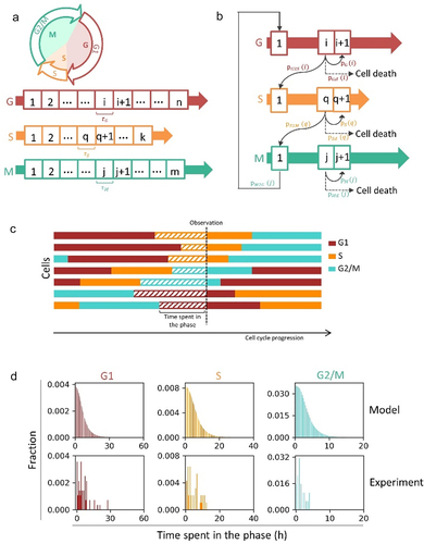
The cells in each bin were modeled by a PBM equation. For cells in each compartment, we modeled them by a set of ordinary differential equations, describing the cells moving in and out of each bin. Assuming the phase durations following lognormal distributions with phase-specific means and variances [12,20], the probabilities of the cells transiting to the first bin of next phase were calculated accordingly. The probability of cell death was simplified as a constant during cell cycle progression. This model captured the key features of heterogeneous proliferating cell, via a relative computational efficient approach (see supplemental materials for details).

Because of the heterogeneity of cell cycle durations, a population always approach to and finally reach a steady state, at which the fractions of cells in each bin are constant and follow a certain distribution. The distribution of steady state could be solved [14]. Here, for simplification, we cultured cells without cell death in silico for a long time (>30 days) until a quasi-steady state was achieved. Interestingly, we found that the cell number in the bin, which describes the number of cells that have spent specific time in the phase (Figure 1c), decreased progressively from the beginning to the end of one compartment (Figure 1d). We validated it using a published experimentally derived dataset [21]. We analyzed the cell cycle progression in the videos of A549 cells expressing a PCNA-mNeonGreen cell cycle reporter (Figure S1A) [21]. The parameters for modeling were estimated by fitting lognormal distributions to the data of phase durations (Figure S1B). Then the distributions of the time spent in the phase of cells at a quasi-steady state were calculated. The results of simulation were in agreement with experimental data (Figure 1d). This specific shape is mainly determined by two factors: one is the continuing noise introduced to the population by the cell division at the end of M phase (one cell divided into two cells); the other is the distribution of phase-transition probabilities.

Modeling quantized cell cycle arrest and graded cell cycle arrest

Next, we introduced cell cycle arrest into the model. Eukaryotic cell cycle duration was characterized as “quantized,” a concept borrowed from quantum physics [22,23]. The histogram of eukaryotic cell cycle durations was a discrete series of interspersed subpopulations (Figures 2a and 3a). The “graded” property of cell cycle arrest was also observed, in response to DNA damage [16]. The duration of cell cycle arrest correlated with the severity of DNA damage (Figures 2b and 3a). To show examples of quantized/graded cell cycle arrest, we used data of live-cell images from previous publication [24]. H358 cells expressing FUCCI biosensor proteins mVenus-hGeminin(1/110) and mCherry-hCdt1(30/120) were treated with 5 µg/ml cisplatin pulse or 1 µM dactolisib pulse for 2 h, then were imaged using confocal microscopy in every 20 min for 72 h. We quantified the cell cycle phase durations of the cells. The durations of G1 phase of cells in response to cisplatin treatment could be described as “quantized” (Figure 2c), while cells responded to dactolisib stimulation in a “graded” way (Figure 2d). Those two typical properties of cell cycle arrest could be characterized in our model. Specifically, permanent arrest could be induced. Cells did not transit within a certain period of time were categorized as permanent arrest. For instance, in a previous study, U2OS cells that did not transit to next cell cycle phase within 48 h were categorized as permanent arrest, although a very small number of transitions could potentially occur after 48 h [16]. In the model, we simulated cells with prolonged phase (longer than experimental duration) to mimic permanent arrest.

Figure 2. Population balance model for cell cycle arrest. (a) Schematic definitions of quantized cell cycle arrest. The histogram of cell cycle durations is a discrete series of interspersed subpopulations. Partial cells are affected by stimulation and the number of cells with prolonged phase increases when cells induced by increasing extent of stimulations. (b) Schematic definitions of graded cell cycle arrest. All cells are affected by stimulation and the cell cycle phase durations become longer when cells induced by increasing extent of stimulations. (c, d) Live-cell images of NCI-H358 cells expressing FUCCI biosensor proteins mVenus-hGeminin(1/110) and mCherry-hCdt1(30/120). Images were taken every 20 min for 72 h under control conditions, or treated with 5 µg/ml cisplatin pulse for 2 h, or treated with 1 µM dactolisib for 2 h. The durations of G1 phase of cells were analyzed. (e, f) Schematic showing the simulation of cell cycle arrest. The phase durations of arrested cells would be lengthened. The length of bins stays the same but the numbers of bins of G1, S, and G2/M phase would change. The probabilities of three conditional fates in one bin of arrested cells would be reassigned. Upon stimulation, cells in one bin would move to the corresponding bins of the affected groups with certain probabilities. After progressing through G’, S’, or M’ phase, cells would move back to the normal cell cycle.

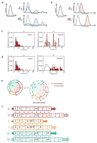
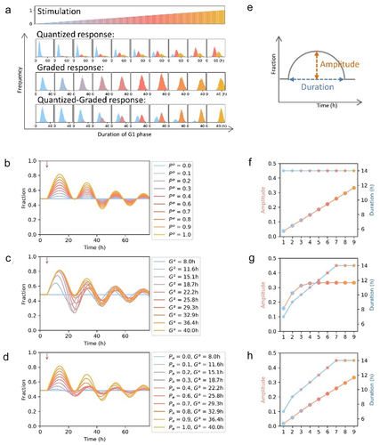
Figure 3. Modeling quantized cell cycle arrest and graded cell cycle arrest. (a) Schematic diagrams for cell cycle arrest at G1 phase induced by increasing extent of stimulations. 10,000 cells were simulated and the cell cycle phase durations were drawn from lognormal distributions (parameters: ${\mu }_G$= 6.15 min, ${\sigma }_G$= 0.22 min, ${\mu }_S$= 5.17 min, ${\sigma }_S$= 0.22 min, ${\mu }_M$= 6.27 min, ${\sigma }_M$= 0.22 min). The cells in G1 phase were affected upon stimulation, and the G1 phase durations of affected cells were drawn from lognormal distributions. Quantized cell cycle arrest: the G1 durations were quantized and fixed. Partial cells were arrested in G1 phase and the affected fraction was proportional to the severity of stimulation. Graded cell cycle arrest: all cells were arrested in G1 phase and the average duration of the G1 phase was adjusted according to the severity of stimulation. Quantized-graded cell cycle arrest: when cells induced by increasing extent of stimulations, the fraction of affected cells increased and the G1 phase durations of affected cells were lengthened. (b) Simulation results of quantized cell cycle arrest. For simplification, only one group of affected cells with fixed lengthened G1 phase durations were modeled in quantized response. The fractions of affected cells increased from 0 to 1. The parameters for the G1 phase of the affected cells: ${{\mu }_G}^{\prime }$= 7.07 min, ${{\sigma }_G}^{\prime }$= 0.22 min. (c) Simulation results of graded cell cycle arrest. The mean of elongated G1 phase durations increased from 8 h to 40 h (Std = 0.22*mean) and the parameters were calculated accordingly. (d) Simulation results of quantized-graded cell cycle arrest. The fractions of affected cells were from 0 to 1 and the mean of elongated G1 phase durations increased from 8 h to 40 h (Std = 0.22*mean), then the parameters were calculated accordingly. Red arrow: timing of stimulation. (e) Schematic definitions of amplitude and duration of the curves. (f–h) Amplitude and duration of quantized, graded, and quantized-graded cell cycle arrest in (b–d), respectively. Circles: amplitude; asterisks: duration. The circles and asterisks correspond to the curves with the same color.

To describe cell cycle arrest, we developed the model by introducing groups of arrested cells (affected groups), of which the cell cycle durations were different. The length of bins of affected groups stays the same but the numbers of bins in G1, S, and G2/M phase would change (Figure 2e). The probabilities of three conditional fates in one bin of arrested cells would be reassigned (see supplemental materials for further details). The stimulation, could be cytokines or stress, triggers a delay in cell cycle. In the model, cells in one bin could move to the corresponding bins of the affected groups with certain probabilities (Figure 2e). After progressing through one G’, S’, or M’ phase, the cell would move back to the normal cell cycle.

We were curious about the population behavior when either quantized cell cycle arrest or graded cell cycle arrest was induced. We show cells arrested in G1 phase as an example (Figure 3a). The cell cycle phase durations were drawn from lognormal distributions. Upon stimulation, cells in G1 phase would be affected and their G1 phase durations were lengthened. We modeled cells responding to increasing severity of stimulation in a quantized, graded, or quantized-graded way. Quantized response: the G1 durations were quantized and fixed. Partial cells were arrested in G1 phase and the affected fraction was proportional to the severity of stimulation. Graded response: all cells were arrested in G1 phase and the average duration of the G1 phase of arrested cells was adjusted according to the severity of stimulation. Quantized-graded response: when cells induced by increasing extent of stimulations, the fraction of affected cells increased and the G1 phase durations of affected cells were lengthened.

We modeled 10,000 cells responding to increasing severity of stimulations in quantized, graded, or quantized-graded way and monitored them for 72 h. For simplification, only one group of affected cells with fixed lengthened G1 phase durations was modeled in quantized response (parameters: ${{\mu }_G}^{\prime }$= 7.07 min, ${{\sigma }_G}^{\prime }$= 0.22 min).

The fraction of cells in G1 phase fluctuated wildly when the graded cell cycle arrest was induced, while the quantized cell cycle arrest resulting in a more organized fluctuation (Figure 3b-–d). We compared the amplitude and duration of the curves describing the fraction of cells in G1 phase (amplitude: the largest difference between the fraction of cells in G1 phase of affected groups and that of control group; duration: the period during which the fraction of cells in G1 phase of affected groups is larger than that of control group; Figure 3e). The amplitudes of the quantized responding groups increased gradually and the durations were constant (Figure 3f). While the amplitudes of the graded responding groups saturated soon and the durations gradually reached the maximum (Figure 3g). Both the amplitudes and durations of the quantized-graded responding groups gradually increased (Figure 3h).

The molecular mechanisms of quantized and graded cell cycle arrest are different. Quantized cell cycle arrest was reported to be related to circadian oscillators [23], while DNA damage-induced cell cycle arrest responded in a graded or graded-quantized pattern [16]. Comparing the characteristics of the simulated data and experimental data could help develop hypotheses efficiently in exploring mechanism of novel cell-cycle-regulating components.

Modeling inheritable cell cycle arrest and experimental validation

Inheritable quiescence from mother cells to daughter cells was reported [25]. The molecular mechanism was that the CDK2 and p21 dynamics during a restriction window at the end of the cell cycle determined the cell fates in next cell cycle [26,27]. TGF-β-induced inheritable cell cycle arrest was observed. Cells in G1 phase are sensitive to TGF-β till reaching a “restriction point.” Cell completed the cell cycle but arrest during the subsequent G1 phase when TGF-β was added after the “restriction point” [28]. We modeled the inheritable cell cycle arrest: the cells in S and G2/M phase upon stimulation would be arrested in the following G1 phase after cell division (Figure 4a). Without inheritable cell cycle arrest, the fraction of cells in G1 phase fluctuated back to initial level in one cell cycle duration (Figure 3b-–d). Once inheritable cell cycle arrest was introduced to the model, the fraction of cells in G1 phase could be larger than initial level for more than two cell cycle duration (Figure 4b-–d).

Figure 4. Modeling inheritable cell cycle arrest. (a) Schematic showing inheritable cell cycle arrest. Immediate arrest was induced when cell stimulated at G1 phase, while cell completed the cell cycle and arrested during the subsequent G1 phase when stimulated at S, G2/M phase. (b) Simulation results of quantized cell cycle arrest. The fractions of affected cells were from 0 to 1. The parameters for the G1 phase of the affected cells: ${{\mu }_G}^{\prime }$= 7.07 min, ${{\sigma }_G}^{\prime }$= 0.22 min. (c) Simulation results of graded cell cycle arrest. The mean of elongated G1 phase durations were from 8 h to 40 h (Std = 0.22*mean) and the parameters were calculated accordingly. (d) Simulation results of quantized-graded cell cycle arrest. The fractions of affected cells were from 0 to 1 and the mean of elongated G1 phase durations were from 8 h to 40 h (Std = 0.22*mean). Red arrow: timing of stimulation.

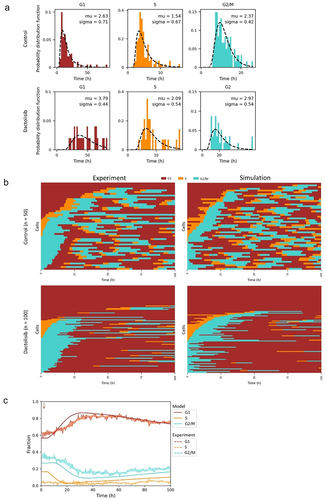
Next, we validated our model using an experimental dataset by Jordan et al. [24]. H358 cells expressing FUCCI were treated with 1 µM dactolisib for 2 h and monitored for 100 h using time-lapse microscopy. We analyzed the images and found an inheritable graded cell cycle arrest was induced. The durations of the cell cycle phases were fitted with lognormal distributions to estimate the parameters $\mu$ and $\sigma$ (Figure 5a). The cell cycle progression was simulated based on the fitted lognormal distribution parameters (Figure 5b). Then we calculated the fractions of cells in G1, S, and G2/M phase, and the results show that the model could capture the oscillatory properties of the experimental data (Figure 5c). We noticed that an increase of the fraction of cells in G1 phase was induced around 3 h after ligand exposure. The delay was considered in the model simulation. Notably, in the model, cells were at the steady state upon stimulation, at which the fractions of cells in each bin and in each cell cycle phase were constant. However, in real world, the cells might slightly deviate from the steady state. Thus, the simulation might not exactly match the experimental data but we still captured the properties and produced the oscillations.

Figure 5. Comparison of experimental data with simulation results. (a) H358 cells expressing FUCCI biosensor proteins mVenus-hGeminin(1/110) and mCherry-hCdt1(30/120) were monitored for 100 h using time-lapse microscopy under control conditions or treated with a dactolisib pulse (1 μM, 2 h). Asynchronously proliferation H358 cells were quantified for their cell cycle phase durations based on the fluorescence of FUCCI. The distributions of the cell cycle phases were fitted with lognormal distributions to estimate parameters (μ, σ). (b) Comparison of simulated cell cycle progression with experimental data. (c) The fractions of cells in G1, S, and G2/M phase after dactolisib treatment were calculated and compared with simulated data. Solid lines: model simulation; dash lines: experimental data. Red arrow: timing of stimulation.

Modeling multiple stimulations and long-term response

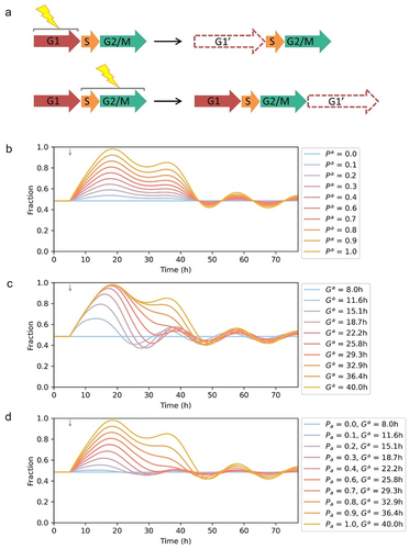
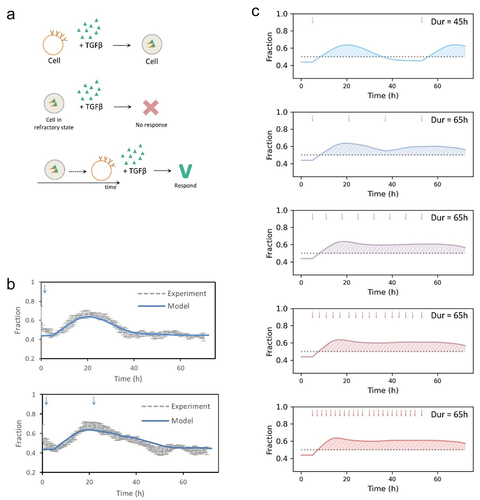
In clinical therapy, multiple treatments are applied and long-term response is crucial to drug resistance. It was known that quiescent cells resist further stress: a refractory state was triggered by a short exposure to TGF-β [29] and quiescent cells would resist DNA damage [30]. We could predict the response of cells to multiple stimulations accounting for refractory periods in our model. We modeled cells treated with TGF-β as an example (Figure 6a). After an initial TGF-β stimulation, cells would be refractory to a further acute stimulus because of the rapid depletion of receptors from the cell surface. Cells recovered from the refractory state and regained response competence to TGF-β in one cell cycle [29]. We modeled cells exposed to a single or double TGF-β stimulation and compared the results with a published experimental dataset [31]. Hacat cells expressing FUCCI biosensor protein mCherry-hGeminin(1/110) were treated with a TGF-β pulse at 0 h (50 pM, 3 h) or double-stimulated with pulses of 50 pM TGF-β at 0 h and 23 h, and were monitored for 72 h using time-lapse microscopy. The distributions of the cell cycle phases of cells under control condition or TGF-β treatments were fitted with lognormal distributions to estimate parameters (μ, σ). We simulated cells in response to a single or double TGF-β stimulation based on the fitted lognormal distribution parameters. The simulations were in agreement with experimental data (Figure 6b). We next modeled cells responding to multiple stimulations and predicted the long-term cell cycle progression (Figure 6c). Interestingly, as the existence of refractory state, cells responded to stimulations with small interval did not induce significantly sustained cell cycle arrest at G1 phase. The results indicated that the timing of stimulations should be considered in long-term treatment.

Figure 6. Modeling multiple stimulations and long-term response. (a) Schematic showing that TGF-β induces a refractory period in which cells are responsiveness to further ligand stimulation. The refractory state is produced because of the rapid depletion of receptors from the cell surface in response to TGF-β binding and their slow replenishment. (b) Comparison of simulated cells in response to a single or double TGF-β stimulation with experimental data. Hacat cells expressing FUCCI biosensor protein mCherry-hGeminin(1/110) were treated with a TGF-β pulse at 0 h (50 pM, 3 h) or double-stimulated with pulses of 50 pM TGF-β at 0 h and 23 h, and were monitored for 72 h using time-lapse microscopy. The parameters were estimated by fitting the distributions of cell cycle phases with lognormal distributions. Cells under control condition: $\tau$= 0.13 h, ${\mu }_G$= 2.07 h, ${\sigma }_G$= 0.22 h, ${\mu }_S$= 1.15 h, ${\sigma }_S$= 0.86 h, ${\mu }_M$= 2.31 h, ${\sigma }_M$= 0.20 h; cells were temporary arrested: ${{\mu }_G}^{\prime }$= 3.27 h, ${{\sigma }_G}^{\prime }$= 0.21 h; cells were permanent arrested: ${{\mu }_G}^{\prime \prime }$= 5.27 h, ${{\sigma }_G}^{\prime \prime }$= 0.22 h. Here we simulated cells with prolonged phase (longer than experimental duration) to mimic permanent arrest. The probability of cells to be temporary arrested upon stimulation: $p_G$=0.29, $p_S$=0.42, $p_M$=0.42; the probability of cells to be permanent arrested: ${p_G}^{\prime }$=0.11, ${p_S}^{\prime }$=0.01, $p_M$’ = 0.01. The time course of recovery from the refractory period was of the order of one cell cycle. Blue arrow: the timing of stimulation. (c) Simulations of cells in response to multiple TGF-β stimulations. The durations that the fraction of cell in G1 phase more than 50% are shown in shadow. Red arrow: timing of stimulation.

Cell cycle synchronization and desynchronization

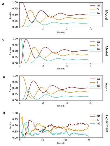
As a number of genes are periodically expressed in the cell cycle, the investigations on molecular events occurring during the cell cycle often require synchronization [32,33]. Several methods were applied to synchronize cultured cells, such as serum deprivation, contact inhibition, and inhibitors of DNA replication. [34,35]. It is important to know the rate of desynchronization after releasing cells from the block. We could estimate it by modeling. We modeled cell cycle synchronization by arresting all cells in the first bin of G1, S, or G2/M phase. After that, the cells were released and cultured for 72 h. Without any further interruptions, the cells would desynchronize and approach to steady state gradually (Figure 7a-–c). Notably, the cells would reach the same steady-state distribution no matter which initial distribution was. The parameters for modeling were estimated from an experimental dataset by Alvaro et al. [21], and the simulated results were compared with the experimental data (Figure 7c, Figure S1B). Cells were synchronized with thymidine and most of them were in early S phase prior to release. Both the experimental data and model output showed that cells desynchronized after two cell cycles. The model showed a good ability to fit to the experimental data. Our model could be applied to predict the rate of desynchronization in future studies.

Figure 7. Modeling synchronization and desynchronization. We modeled cell cycle synchronization by arresting all cells in the first bin of G1 phase (a), G2/M phase (b), or S phase (c) then releasing cells progressing at same rate as normal cell cycle progression. The parameters were estimated from the experiments by fitting lognormal distributions to the data of phase durations (${\mu }_G$= 2.08 h, ${\sigma }_G$= 0.60 h, ${\mu }_S$= 2.02 h, ${\sigma }_S$= 0.55 h, ${\mu }_M$= 1.40 h, ${\sigma }_M$= 0.53 h). G1, S and G2/M phases were divided into 500, 613, and 561 bins, respectively. The probabilities of cell death were set as 0. The probabilities of the other two cell fates, transiting to the next cell cycle phase or moving to the next bin, were calculated accordingly. (d) A549 cells expressing PCNA cell cycle reporter were synchronized with thymidine and released for 2 h to enrich for early S phase-target cells, then were imaged using confocal microscopy in every 30 min for 72 h.

Discussion

Cell cycle control is essential to normal activities for living organisms. In response to stress or stimulations, cells may arrest at a specific cell cycle stage. In clinical treatment, understanding the population cell cycle kinetics is key to cell-cycle-sensitive drug delivery or therapy application. In this study, we developed a mathematical model of cell cycle control and deconvoluted the population kinetics through a computational approach. The model provided a successfully representation of the cell cycle kinetics. We modeled three typical cell cycle arrest: quantized, graded, or quantized-graded response. Then we illustrated the effect of different response pattern on the dynamics of the population. Our model could describe inheritable quiescence and refractory state, which were crucial in long-term response of the population. Then, we monitored cells responding to multiple stimulations, which could be used to provide information for deciding intervals of experimental treatments. Our model addressed the population behavior in response to stress or cytostatic cytokines, being useful in studies or clinical therapies related to cell cycle arrest.

Our data showed that a population always approach to and finally reach a steady state, at which the fractions of cells in each bin are constant. Intuitively, one might assume a uniform distribution of cell numbers at each stage of the cell cycle. However, via model simulation, we found that the cell number in the bin decreased progressively from the beginning to the end of one compartment. The explanation to this counterintuitive result was that the probabilities of the cell, instead of the cell number, located at each stage of a cell cycle followed the uniform distribution. The population kept growing and cells divided into two at the end of the M phase, resulting in this special distribution of the cell numbers in each bin. The cell cycle phase durations were described as lognormal distributed [36,37]. Coincidentally, proteins were also lognormal distributed across the population [38,39]. One intuitive assumption would be that the level of one constantly accumulating protein dominantly governs the phase transition. A following question is which one dominantly determines the duration. As many proteins are involved in the cell phase duration regulation and their functions are redundant, unraveling their relationship and the molecular mechanism of cell cycle regulations is still needed to answer this question.

The molecular mechanisms of two typical properties of cell cycle arrest, quantized and graded, are different. The quantized response could be the result of a self-sustaining signaling activation system, toggling between “on” or “off” states achieved by positive feedback circuits or double-negative feedback circuits [40]. The Myc/Rb/E2F network was proposed to control the commitment decision of cell cycle and CDK2/p21 circuit was also reported to control the proliferation-to-quiescence decision [41]. It will be interesting to investigate and combine those two systems to better understand the cell cycle regulation. The graded response refers to the graded increased level of transcriptional activity determined by the number of occupied binding sites [42]. G1 cyclin/CDKs were demonstrated to control the timing in cell cycle progression [41]. Our model could simulate population behavior according to the specific properties of cell cycle arrest to predict long-term cellular response; conversely, it also provided an application to infer molecular mechanism efficiently from responding profiles at population level.

The cell cycle arrest regulation is complicate, involving different responding patterns, inheritable quiescence, multiple stimulations, and refractory state of cells. Our model could incorporate several influence factors and predict the long-term fluctuation of the number of cells in each cell cycle state, providing a powerful tool to uncover mechanisms for observations and offer suggestions on therapeutics.

Authors’ contributions

GW: conceptualization, implementation, investigation, image analysis, writing, editing, and revising the manuscript. YL: investigation, editing, and revising the manuscript. HX, HL, and YD: image analysis. All authors read and approved the final manuscript.

Ethics approval and consent to participate

Not applicable.

Consent for publication

Not applicable.

Data accessibility statement

The data that support the findings of this study are available from the corresponding author upon reasonable request.

Acknowledgments

The authors would like to acknowledge Dr. David R Croucher and Dr. Andrew Burgess for provision of the microscopy data of cells expressing a FUCCI or PCNA-mNeonGreen cell cycle reporter. This study was supported by National Key Clinical Specialty Construction Project (Clinical Pharmacy) and High Level Clinical Key Specialty (Clinical Pharmacy) in Guangdong Province. This study was also supported by the Construction Project of NMPA Key Laboratory for Technology Research and Evaluation of Pharmacovigilance.

Disclosure statement

No potential conflict of interest was reported by the author(s).

Supplementary material

Supplemental data for this article can be accessed here

Additional information

Funding

This study was supported by National Key Clinical Specialty Construction Project (Clinical Pharmacy) and High Level Clinical Key Specialty (Clinical Pharmacy) in Guangdong Province. This study was also supported by the Construction Project of NMPA Key Laboratory for Technology Research and Evaluation of Pharmacovigilance.

References

- Siegel PM, Massague J. Cytostatic and apoptotic actions of TGF-beta in homeostasis and cancer. Nat Rev Cancer. 2003;3(11):807–821.
- Hanahan D, Weinberg RA. Hallmarks of cancer: the next generation. Cell. 2011;144(5):646–674.
- Hustedt N, Durocher D. The control of DNA repair by the cell cycle. Nat Cell Biol. 2016;19(1):1–9.
- Engeland K. Cell cycle arrest through indirect transcriptional repression by p53: i have a DREAM. Cell Death Differ. 2018;25(1):114–132.
- Massague J. TGFbeta signalling in context. Nat Rev Mol Cell Biol. 2012;13(10):616–630.
- Strzyz P. Cell signalling: signalling to cell cycle arrest. Nat Rev Mol Cell Biol. 2016;17(9):536.
- Min M, Spencer SL. Spontaneously slow-cycling subpopulations of human cells originate from activation of stress-response pathways. PLoS Biol. 2019;17(3):e3000178.
- Gookin S, Min M, Phadke H, et al. A map of protein dynamics during cell-cycle progression and cell-cycle exit. PLoS Biol. 2017;15(9):e2003268.
- Gerard C, Goldbeter A. Temporal self-organization of the cyclin/Cdk network driving the mammalian cell cycle. Proc Natl Acad Sci U S A. 2009;106(51):21643–21648.
- Sible JC, Tyson JJ. Mathematical modeling as a tool for investigating cell cycle control networks. Methods. 2007;41(2):238–247.
- Barr AR, Heldt FS, Zhang T, et al. A dynamical framework for the all-or-none G1/S transition. Cell Syst. 2016;2(1):27–37.
- Altinok A, Levi F, Goldbeter A. A cell cycle automaton model for probing circadian patterns of anticancer drug delivery. Adv Drug Deliv Rev. 2007;59(9–10):1036–1053.
- Altinok A, Gonze D, Levi F, et al. An automaton model for the cell cycle. Interface Focus. 2011;1(1):36–47.
- Fuentes-Gari M, Misener R, Garcia-Munzer D, et al. A mathematical model of subpopulation kinetics for the deconvolution of leukaemia heterogeneity. J R Soc Interface. 2015;12(108):20150276.
- Fuentes-Garí M, Misener R, Georgiadis MC, et al. Selecting a differential equation cell cycle model for simulating leukemia treatment. Ind Eng Chem Res. 2015;54(36):8847–8859.
- Chao HX, Poovey CE, Privette AA, et al. Orchestration of DNA damage checkpoint dynamics across the human cell cycle. Cell Syst. 2017;5(5):445–459 e445.
- Bartlett TE, Muller S, Diaz A. Single-cell co-expression subnetwork analysis. Sci Rep. 2017;7(1):15066.
- Singhania R, Sramkoski RM, Jacobberger JW, et al. A hybrid model of mammalian cell cycle regulation. PLoS Comput Biol. 2011;7(2):e1001077.
- Crosby ME. Cell cycle: principles of control. Yale J Biol Med. 2007;80(3):141–142.
- Dowling MR, Kan A, Heinzel S, et al. Stretched cell cycle model for proliferating lymphocytes. Proceedings of the National Academy of Sciences of the United States of America 2014, 111( 17):6377–6382.
- Gonzalez Rajal A, Marzec KA, McCloy RA, et al. A non-genetic, cell cycle-dependent mechanism of platinum resistance in lung adenocarcinoma. Elife. 2021;10. DOI:https://doi.org/10.7554/eLife.65234.
- Klevecz RR. Quantized generation time in mammalian cells as an expression of the cellular clock. Proc Natl Acad Sci U S A. 1976;73(11):4012–4016.
- Arata Y, Takagi H. Quantitative studies for cell-division cycle control. Front Physiol. 2019;10:1022.
- Hastings JF, Gonzalez Rajal A, Latham SL, et al. Analysis of pulsed cisplatin signalling dynamics identifies effectors of resistance in lung adenocarcinoma. Elife. 2020;9. DOI:https://doi.org/10.7554/eLife.53367.
- Arora M, Moser J, Phadke H, et al. Endogenous replication stress in mother cells leads to quiescence of daughter cells. Cell Rep. 2017;19(7):1351–1364.
- Spencer SL, Cappell SD, Tsai FC, et al. The proliferation-quiescence decision is controlled by a bifurcation in CDK2 activity at mitotic exit. Cell. 2013;155(2):369–383.
- Moser J, Miller I, Carter D, et al. Control of the restriction point by Rb and p21. Proc Natl Acad Sci U S A. 2018;115(35):E8219–E8227.
- Donovan J, Slingerland J. Transforming growth factor-beta and breast cancer: cell cycle arrest by transforming growth factor-beta and its disruption in cancer. Breast Cancer Res. 2000;2(2):116–124.
- Vizan P, Miller DS, Gori I, et al. Controlling long-term signaling: receptor dynamics determine attenuation and refractory behavior of the TGF-beta pathway. Sci Signal. 2013;6(305):ra106.
- Brown JA, Yonekubo Y, Hanson N, et al. TGF-beta-induced quiescence mediates chemoresistance of tumor-propagating cells in squamous cell carcinoma. Cell Stem Cell. 2017;21(5):650–664 e658.
- Wu G. Single cell analysis reveals all-or-none G1 arrest decisions upon TGFβ stimulation. Berlin: Humboldt-Universität zu; 2019.
- Cho RJ, Huang M, Campbell MJ, et al. Transcriptional regulation and function during the human cell cycle. Nat Genet. 2001;27(1):48–54.
- Whitfield ML, Sherlock G, Saldanha AJ, et al. Identification of genes periodically expressed in the human cell cycle and their expression in tumors. Mol Biol Cell. 2002;13(6):1977–2000.
- Davis PK, Ho A, Dowdy SF. Biological methods for cell-cycle synchronization of mammalian cells. Biotechniques. 2001;30(6):1322–1326. 1328, 1330-1321.
- Kurose A, Tanaka T, Huang X, et al. Synchronization in the cell cycle by inhibitors of DNA replication induces histone H2AX phosphorylation: an indication of DNA damage. Cell Prolif. 2006;39(3):231–240.
- Liu D, Umbach DM, Peddada SD, et al. A random-periods model for expression of cell-cycle genes. Proc Natl Acad Sci U S A. 2004;101(19):7240–7245.
- Dowling MR, Kan A, Heinzel S, et al. Stretched cell cycle model for proliferating lymphocytes. Proc Natl Acad Sci U S A. 2014;111(17):6377–6382.
- Spencer SL, Gaudet S, Albeck JG, et al. Non-genetic origins of cell-to-cell variability in TRAIL-induced apoptosis. Nature. 2009;459(7245):428–432.
- Sigal A, Milo R, Cohen A, et al. Variability and memory of protein levels in human cells. Nature. 2006;444(7119):643–646.
- Ferrell JE Jr. Self-perpetuating states in signal transduction: positive feedback, double-negative feedback and bistability. Curr Opin Cell Biol. 2002;14(2):140–148.
- Dong P, Maddali MV, Srimani JK, et al. Division of labour between Myc and G1 cyclins in cell cycle commitment and pace control. Nat Commun. 2014;5(1). DOI:https://doi.org/10.1038/ncomms5750
- Kringstein AM, Rossi FM, Hofmann A, et al. Graded transcriptional response to different concentrations of a single transactivator. Proc Natl Acad Sci U S A. 1998;95(23):13670–13675.