On-demand driver vigilance enhancement without explicit drowsiness detection—Further analysis of the pilot study results

ABSTRACT

Objective: A new active safety concept that engages the driver's psychosensory pain-processing mechanism to automatically trigger vigilance enhancement on-demand was proposed in Chang (2012). This concept is based on the hypothesis that a human's pain threshold will decline as he or she becomes drowsy, consequently triggering the vigilance enhancer. The objective of this pilot study was to develop methods to test this hypothesis, the results of which could lead to further refinement of the hypothesis and methods, with the ultimate goal of developing new active safety concepts that exploit the driver's endogenous psychosensory pain-processing mechanisms. Preliminary results from a pilot study designed to test this hypothesis were presented in Chang (2016). This article presents further analysis of the pilot study data.

Methods: Perceived pain responses of six healthy male participants were measured when their vigilance would be under stress. A time-varying thermal grill illusion (TGI) of pain was created using a custom steering wheel with an array of Peltier elements held in the participant's palm. The participant's pain responses to the TGI stimulus were recorded while changes in his vigilance were monitored using pre- and post-session Psychomotor Vigilance Task (PVT) tests, in-session Percent Eyelid Closure (PERCLOS), and subjective Karolinska Sleepiness Scale (KSS) ratings. The probability of pain response versus TGI temperature stimulus and vigilance measures were then estimated using logistic regression analysis.

Results: The results indicate that the probability of pain response is correlated with the temperature stimuli and the vigilance state. The pain threshold tends to move up or down versus KSS depending on the participant for high-vigilance conditions, but tends to increase when the participant becomes increasing drowsy in low-vigilance conditions. These results were statistically significant for four of the six study participants.

Conclusions: This limited pilot study observed that one's pain threshold may or may not initially decrease as originally hypothesized depending on the participant, but then increases as one becomes drowsier. While not definitive, the methods and results of this study may help to refine our hypotheses and design future studies in pursuit of detector-free on-demand driver vigilance enhancement that exploits our body's endogenous alert mechanism.

KEYWORDS:

• Drowsiness
• Karolinska Sleepiness Scale
• Peltier
• thermal grill illusion
• vigilance

Introduction

Drowsy driving is a major hazard for our society. It has been estimated that more than 100,000 vehicular crashes per year in the United States involve drowsy driving (Tefft 2014). Therefore, some form of intervention is necessary when a driver shows signs of drowsiness.

Technologies developed thus far typically involve some type of drowsiness detection and intervention that is external to the driver. Drowsiness detection can be based on ocular or other measures. Interventions can include a reminder to take a rest break or an alert to wake up the driver. The effects of these interventions are usually temporary in nature. This detect-and-intervene paradigm can produce false alarms that lead to distrust and disengagement (e.g., Blanco et al. 2009), which does not promote driver acceptance. False negatives can also put road users in peril when drivers become accustomed to being awakened and their danger sensing capabilities atrophy.

This presents challenges and opportunities for researchers. We set out to investigate a new way to tackle this problem, inspired by the observation that sleep debt is such an acute stressor to our bodies that it demands a high-priority response in our behavior. Few factors come as close other than our body's internal temperature and pain sensation. For example, it is often difficult to fall asleep when we feel pain or our body aches. Can we then leverage our body's internal defense mechanisms to our benefit, so that we don't fall asleep when we are at the wheel? If the answer is yes, then this could lead to a new driver vigilance enhancement approach that is potentially superior or complimentary to external detect-and-intervene approaches because it relies on one's endogenous danger detection, and when activated and the resulting vigilance enhancement is attained, the response automatically subsides into the background (for full details see Chang 2012).

For this new approach to work we need to test an important hypothesis that our body's pain threshold will decline as we become drowsy. In the sleep medicine literature and the pain medicine literature we see hints that this threshold is at different set points when one is awake or asleep, and consequently one reacts to pain differently in those states. Our inspiration is to find out whether such changes in pain perception can be modeled with vigilance or drowsiness as an independent variable.

Objectives

The objectives of the pilot study and the analysis presented herein was to investigate the effects of low driver vigilance on the probability of perceiving pain resulting from a variable thermal grill illusion (TGI) (Green 2002; Lindstedt et al. 2011). The original hypothesis inspired by prior sleep research is that the human's pain threshold will decline, and therefore the probability of perceiving pain will increase, as he or she becomes drowsy, similar to hypersensitivity to pain observed in sleep-deprived patients (Onen et al. 2001).

Methods

This pilot study involved experimentally stimulating and recording perceived pain responses from six healthy adult males to a range of TGI events under a range of vigilance conditions, in order to estimate empirical models for the probability of pain perception in terms of sleepiness ratings and objective measures. These models can then be used to describe the effect of sleepiness on pain threshold.

Experimental approach

The experimental approach involved stimulating and recording perceived pain responses using the pain stimulus, test device, and experimental matrix summarized herein. The testing protocols used in this study were approved by the Dynamic Research, Inc. (DRI) Institutional Review Board (Department of Health and Human Services [DHHS] registration number IRB 00006962) before the participant testing was conducted. Additional information is in Appendix A (see online supplement) and Chang (2016).

Stimulus and test device

Changes in the perception of pain were the main outcome of interest in this study (in contrast to vigilance, which was the main input of interest). The illusion of pain was stimulated using a custom-designed “hand unit” resembling a fixed steering wheel incorporating a 3 × 5-element Peltier array located under the palm of the participant's right hand (Figure 1). The Peltier array was designed to produce time-varying warm and cold temperatures in adjacent elements in order to create an illusion of pain.

Figure 1. Prototype steering wheel with Peltier array and buttons to report the KSS rating (the button to report pain is not shown).

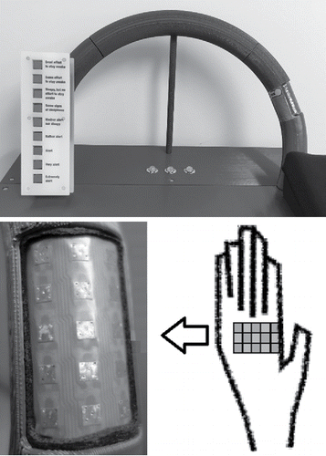
Perceived pain and subjective Karolinska Sleepiness Scale (KSS) ratings (Åkerstedt et al. 2014) were recorded using buttons located near the hand unit, as shown in Figure 1. The KSS ratings were reported by pressing one of nine buttons labeled with sleepiness rating adjectives, and the corresponding integer values 1 through 9 were recorded (Table A4; see online supplement). The vigilance of the participant was also monitored using a pre- and post-session Psychomotor Vigilance Task (PVT; Khitrov 2014) and a Percent Eyelid Closure (PERCLOS; Grace and Steward 2001) monitoring device placed in front of the participant to objectively measure eye closures during the test sessions. Video showing the nominal face and hand positions of the test participants were also recorded for diagnostic purposes.

Experimental matrix

The experimental matrix for the pilot study comprised six healthy adult male participants, each of whom was nominally tested on three separate days (evenings), with two back-to-back 45-min sessions per day (evening). Each participant had right hand preference, corresponding to the location of the Peltier array on the hand unit. During each session the participant was stimulated with a 5 second TGI event followed by a thermal “resting” period (when all Peltier elements would be set to palm temperature) of approximately 10 s. Each TGI event had a commanded warm and cold Peltier array temperature that was randomly independently sampled from a uniform distribution (e.g., Figure B2; see online supplement). The participant was instructed to press the pain button if he perceived pain during the TGI event. The participant was also prompted to press a KSS rating button every 5 min during the session. Each of the testing days was nominally separated from the next by one or more days to provide for rest. The back-to-back sessions were separated by a 15-min break. The experimental matrix and testing protocols are described in further detail in Appendix A (see online supplement) and Chang (2016).

Event data reduction and data screening

Data describing the individual TGI events were determined from the time domain data recorded for each session. This was accomplished by first identifying the start and stop time for each TGI event based on the difference between the maximum and minimum Peltier array temperature values (T_gap ⩾ 6°C). The resulting identified events for an example session are shown in Figure B1 (see online supplement).

Data for vigilance metrics and KSS ratings for each TGI event were also determined by interpolation or extrapolation to the event times (Figure B3; see online supplement). If the participant did not report a KSS rating within 10 s of being prompted (by a light-emitting diode [LED] according to the test instructions), then the video of the participant during this time interval was reviewed to determine why. If the participant appeared to be asleep then the KSS rating was assumed to be 10, which is an extension to the traditional KSS scale (Table A4; see online supplement); otherwise, the KSS rating was treated as a “missing value.” The most likely KSS rating at the time of each TGI event (KSS_ml) was then estimated by interpolating or extrapolating the numerical KSS ratings to the event times and then rounding the results to the nearest integer value. The integer values correspond to the rating-scale adjectives.

The participants were instructed to press a button if they perceived any pain with their hand that was in contact with the Peltier device. The participant may or may not perceive any pain and press the button, depending on the Peltier array temperatures used to create the TGI event (Green 2002), his or her vigilance, and perhaps other factors. The reported painful ratings were then matched to the corresponding TGI stimulus events. A “painful” database variable was assigned a value of 1 for each TGI stimulus event with a reported painful rating; otherwise, the variable was assigned a value of 0. TGI events with no reported pain were presumably below the pain threshold.

The database was then screened to exclude data from sessions with less than three reported KSS ratings because there were insufficient data to track any fluctuating changes in the participant's vigilance during the session. This exclusion only affected the data for participant 1917 (Table A2; see online supplement).

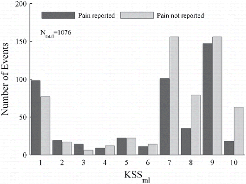
Figure 2 illustrates the number of events (1076) for participant 1232 versus KSS_ml. The numbers of events with and without reported pain for each KSS_ml value are indicated by a pair of vertical bars. The bar on the right side of each pair indicates the number of events with reported pain. The bar on the left indicates the number of events without reported pain.

Figure 2. Example number of events recorded and used in the analysis, by reported pain and KSS rating (participant 1232).

Candidate models and statistical analysis

It was assumed that the probability of a participant reporting pain in this pilot study was a function of the minimum and maximum Peltier temperatures during each TGI event, the participant's vigilance, and potentially other factors. For the purpose of this analysis it was assumed that the probability of reporting pain in each TGI event can be expressed by the following equation: (1) $$\begin{array}{c}\hfill P\left(\mathrm{reported}\mathrm{pain}\right)=P\left(\mathrm{y}=1\right)=\pi \left({\beta }_0+\sum _i{\beta }_i{x}_i\right)\end{array}$$(1) where (2) $$\begin{array}{c}\hfill \pi \left(q\right)\widehat{=}\frac{e^q}{1+e^q}\end{array}$$(2) (3) $$\begin{array}{c}\hfill x_1=T_{\mathrm{gap}}=T_{max}-T_{min}\\ \hfill x_2=T_{min}\\ \hfill x_3=KS{S}_{ml}\\ \hfill x_4=KS{S}_{ml}^2\\ \hfill x_5=Da{y}_1\\ \hfill ⋮\\ \hfill x_8=Da{y}_4\\ \hfill x_9=Sessio{n}_2\\ \hfill x_{10}=t_s\end{array}$$(3) and where

y = 1	=	if the participant reported pain during the event, otherwise y = 0;
π(q)	=	is the inverse of the logit function, which has a unique and continuous mapping between − ∞ < q < ∞ and 0 < π(q) < 1;
Dayj = 1	=	if the event occurred during the j th day of testing for the participant, otherwise Dayj = 0;
Session2 = 1	=	if the event occurred during the second session of the day for the participant, otherwise Session2 = 0; and
ts	=	is the time in hours since the start of the session.

The T_gap and T_min terms^{Figure 2}quantify the TGI stimulus event. The KSS_ml and KSS²_ml terms quantify the participant's vigilance at the time of the event, allowing for possible nonlinear trends. The Day_i terms allow for possible day-to-day differences in the participant's pain threshold due factors such as the amount and quality of sleep, meals and other activities prior to the test sessions, and longer term pain adaptation effects. The Session₂ and t_s terms allow for possible short-term pain adaptation and sensitization. Note that the Day_i, Session₂, and t_s terms represent the net combined effects of potential confounds, which may move the pain threshold in opposite directions and cancel each other out in these data.

PVT and PERCLOS are measures of driver vigilance that were also initially considered for the candidate models. The PVT data were not used because they were only recorded pre- and post-session, and therefore interpolation to the TGI event times would not track any fluctuating changes in driver vigilance during the session (e.g., Figure B3; see online supplement). The PERCLOS data were not used because there were intermittent time intervals where the camera did not detect the participant's eyes. A review of the video data indicated that these data dropouts were due to factors such as head motion and eyewear (Appendix A; see online supplement).

The values for β_i in Eq. (1(1) $$\begin{array}{c}\hfill P\left(\mathrm{reported}\mathrm{pain}\right)=P\left(\mathrm{y}=1\right)=\pi \left({\beta }_0+\sum _i{\beta }_i{x}_i\right)\end{array}$$(1) ) are unknown but can be estimated from the data for each participant using logistic regression analysis (Hosmer et al. 2013). The logistic regressions were accomplished using the Generalized Linear Model implemented in the MATLAB Statistics Toolbox “glmfit” routine, and assuming that y has a binominal distribution with a “logit” link function (Mathworks 2006).

Candidate models for each participant included all (e.g., 720) combinations of the terms in Eq. (3(3) $$\begin{array}{c}\hfill x_1=T_{\mathrm{gap}}=T_{max}-T_{min}\\ \hfill x_2=T_{min}\\ \hfill x_3=KS{S}_{ml}\\ \hfill x_4=KS{S}_{ml}^2\\ \hfill x_5=Da{y}_1\\ \hfill ⋮\\ \hfill x_8=Da{y}_4\\ \hfill x_9=Sessio{n}_2\\ \hfill x_{10}=t_s\end{array}$$(3) ) that meet the following criteria:

•	The model includes one or more of the KSSml terms because KSS is the main variable of interest.
•	The model does not include all of the Dayj terms because one of the Dayj terms is redundant.

The β_i values for the terms that are not in the candidate model are effectively equal to 0.

Logistic regressions were then accomplished for all of the candidate models using the data from each participant. The results for each candidate participant model include:

1.	The regression coefficients (bi), which are the maximum likelihood estimates of βi.
2.	The Wald standard errors ($s_{b_i}$) of bi.
3.	The deviance (4) $$\begin{array}{c}\hfill D=-2\sum _{k=1}^n\left(y_{k}ln\left({\widehat{y}}_k\right)+\left(1-y_k\right)ln\left(1-{\widehat{y}}_k\right)\right)\end{array}$$(4) where the estimated probability of reported pain is (5) $$\begin{array}{c}\hfill \widehat{P}\left(\mathrm{reported}\mathrm{pain}\right)=\widehat{y}=\pi \left(b_0+\sum _{i=1}^p{b}_i{x}_i\right)\end{array}$$(5)
4.	The Bayesian Information Criterion (BIC; Allison 1999), (6) $$\begin{array}{c}\hfill BIC=D+pln\left(n\right)\end{array}$$(6) where n is the number of observations (i.e., TGI events) and p is the number of terms in the model.

The 95% confidence intervals for the regression coefficients are $b_i\pm 1.96s_{b_i}$. The regression coefficients are considered to be statistically significant at the 0.05 level of probability if $|b_i|>1.96s_{b_i}$. The deviance is a measure of the model fit, which the logistic regression seeks to minimize.

The candidate model with the smallest BIC value for each participant was then selected as the “best” model. This model will tend to be parsimonious with a small but not necessarily the minimum possible deviance.

Results

We begin with the logistic regression model search results for participant 1232. The candidate model for this participant with the smallest BIC value had T_min, KSS_ml, KSS²_ml, Day₁, and Day₃ terms. The other candidate terms are not included in this model because the BIC value would increase, indicating possible overparameterization, which is undesirable. Likewise, models with fewer terms also had larger BIC values because the fit was not as good. The deviance and BIC values for this model are 1289.2 and 1331.0, respectively. These figures of merit are much better than, for comparison, the deviance and BIC values of 1464.5 and 1478.5, respectively, for a model with only T_gap (note that a model with only T_gap was also not considered further because it does not include KSS_ml, which is the main variable of interest).

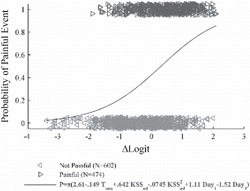
The graph in Figure 3 illustrates the fit of the minimum BIC model to the painful rating data for participant 1232. There were 602 not-painful and 474 painful events used in this analysis, as indicated in Figure 2. The vertical axis of this graph is the probability of a painful rating. The reported ratings are plotted with “◃” and “▹” symbols with the vertical coordinate at either 0 (no reported pain) or 1 (reported pain), respectively. The vertical coordinates of the symbols have been “jittered” by adding a uniformly distributed random number between −0.05 and 0.05 to better illustrate the data distribution (Hosmer et al. 2013). The horizontal axis of this graph is (7) $$\begin{array}{c}\hfill \Delta Logit=\sum _{i=1}^p{b}_i\left(x_i-{\bar{x}}_i\right)=\sum _{i=1}^p{b}_i\Delta x_i\end{array}$$(7)

Figure 3. Example minimum BIC logistic regression model fit (participant 1232).

where ${\bar{x}}_i$ is the mean value for x_i in the event data. Therefore, ΔLogit = 0 when $x_i={\bar{x}}_i$. The estimated probability of pain can then be expressed as $\widehat{y}=\pi \left(b_0^{*}+\Delta Logit\right)$, where $b_0^{*}=b_0+{\sum }_{i=1}^p{b}_i{\bar{x}}_i$. The solid curve is the estimated probability of reported pain based on these equations. Note that ΔLogit depends on the participant model, and b*₀ depends on the overall percentage of TGI events that the participant reported as painful. The range of the probability of pain predicted by this model over the domain of the data is greater than 0.8.

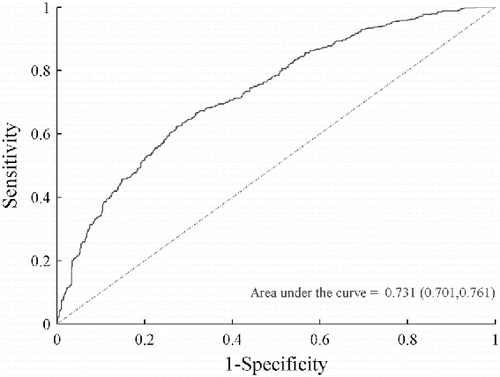
The Receiver Operating Characteristic (ROC) curve for this model is depicted in Figure 4. The diagonal reference line indicates the expected results for a model with no ability to discriminate between painful and not-painful ratings. The area under this reference line is 0.5. The curve located above the diagonal reference line indicates the ability of the minimum BIC model to discriminate between painful and not-painful ratings. The area under the ROC curve for this model is 0.731 (0.701, 0.761), which is statistically significantly greater than 0.5. Guidelines in Hosmer et al. (2013) consider this to be acceptable discrimination.

Figure 4. Receiver Operating Characteristic (ROC) curve for the example minimum BIC logistic regression model (participant 1232).

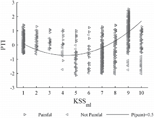
Figure 5 illustrates a scatter plot of event rating data versus KSS_ml, which is the main variable of interest. Not-painful and painful ratings for each TGI event are indicated by the “◃” and “▹” symbols. The horizontal and vertical coordinates for each rating are KSS_ml and PTI calculated according to following equation: (8) $$\begin{array}{c}\hfill PTI=\sum _{i\notin \left\{KS{S}_{\mathrm{ml}},KS{S}_{ml}^2\right\}}{b}_i\left(x_i-{\bar{x}}_i\right)=\sum _{i\notin \left\{KS{S}_{\mathrm{ml}},KS{S}_{ml}^2\right\}}{b}_i\Delta x_i\end{array}$$(8)

Figure 5. Example pain threshold trend versus KSS (participant 1232).

PTI is similar to ΔLogit but does not include the KSS_ml terms. PTI = 0 when T_min and the other control variables (e.g., Day_i) are equal to their respective mean database values.

The curve in Figure 5 is the PTI value where the estimated probability of reported pain is 0.5. By algebraic manipulation of Eqs. (2(2) $$\begin{array}{c}\hfill \pi \left(q\right)\widehat{=}\frac{e^q}{1+e^q}\end{array}$$(2) ), (3(3) $$\begin{array}{c}\hfill x_1=T_{\mathrm{gap}}=T_{max}-T_{min}\\ \hfill x_2=T_{min}\\ \hfill x_3=KS{S}_{ml}\\ \hfill x_4=KS{S}_{ml}^2\\ \hfill x_5=Da{y}_1\\ \hfill ⋮\\ \hfill x_8=Da{y}_4\\ \hfill x_9=Sessio{n}_2\\ \hfill x_{10}=t_s\end{array}$$(3) ), (5(5) $$\begin{array}{c}\hfill \widehat{P}\left(\mathrm{reported}\mathrm{pain}\right)=\widehat{y}=\pi \left(b_0+\sum _{i=1}^p{b}_i{x}_i\right)\end{array}$$(5) ), and (8(8) $$\begin{array}{c}\hfill PTI=\sum _{i\notin \left\{KS{S}_{\mathrm{ml}},KS{S}_{ml}^2\right\}}{b}_i\left(x_i-{\bar{x}}_i\right)=\sum _{i\notin \left\{KS{S}_{\mathrm{ml}},KS{S}_{ml}^2\right\}}{b}_i\Delta x_i\end{array}$$(8) ), it can be shown that the equation for this curve is (9) $$\begin{array}{c}\hfill PT{I}_{\widehat{y}=0.5}=-b_0-b_{3}KS{S}_{ml}-b_{4}KS{S}_{ml}^2\end{array}$$(9) where $PT{I}_{\widehat{y}=0.5}$ is defined such that (10) $$\begin{array}{ccc}\hfill \widehat{P}\left(\mathrm{reported}\mathrm{pain}\right)& =& \pi \left(b_0+PTI+b_{3}KS{S}_{ml}+b_{4}KS{S}_{ml}^2\right)\hfill \\ & & \left\{\begin{array}{ccc}\hfill >0.5& \hfill \mathrm{if}& \hfill PTI>PT{I}_{\widehat{y}=0.5}\\ \hfill =0.5& \hfill \mathrm{if}& \hfill PTI=PT{I}_{\widehat{y}=0.5}\\ \hfill <0.5& \hfill \mathrm{if}& \hfill PTI<PT{I}_{\widehat{y}=0.5}\end{array}\right.\hfill \end{array}$$(10)

An increase in $PT{I}_{\widehat{y}=0.5}$ corresponds to a decrease in the probability of pain for a given PTI value, which can be attributed an increase in the pain threshold. Therefore $PT{I}_{\widehat{y}=0.5}$ can be interpreted as surrogate measure of the pain threshold. These results indicate that the perceived pain threshold decreased when the vigilance of this participant changed from KSS = 1 (extremely alert) to KSS = 5 (not alert/sleepy), but then increased when he became more drowsy to KSS = 10 (asleep).

Results for the minimum BIC model for each participant are located in Appendix C (see online supplement). This includes graphical results similar to Figure 3, Figure 4, and Figure 5 for each of the participant models. Numerical results are listed in Table C1 (see online supplement). The areas under the ROC curves are all statistically significantly greater than 0.5 with values between 0.73 and 0.88, which according to Hosmer et al. (2013) indicates acceptable to excellent discrimination.

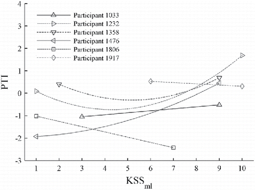
The estimated pain threshold results for all of the participants are summarized in Figure 6. The regression coefficients that describe these trends were statistically significant for all of the participants except participant 1917. The results for participant 1917 were not statistically significant due to the limited amount of KSS data for this participant, and are not further discussed herein. The $PT{I}_{\widehat{y}=0.5}$ values, which are based on different model coefficients for each participant, are generally consistent with the overall percentages of painful events reported by the individual participants. For example, participant 1232 reported pain in 44% (474/1076) of the events and has relatively high $PT{I}_{\widehat{y}=0.5}$ values, which tend to be clustered near KSS_ml= 1, 7, and 9. In contrast, participant 1806 reported pain in 77% (612/798) of the events and has relatively low $PT{I}_{\widehat{y}=0.5}$ values.

Figure 6. Summary of pain threshold versus KSS results based on all of the data.

Models for four of the six participants were also estimated using a subset of the data as a sensitivity analysis to potential confounding factors. This data excluded:

•	Alert and high-vigilance conditions, defined as KSSml < 5.
•	Asleep condition, defined herein as KSSml = 10.
•	Sessions where more than 15% of the events had Tgap ⩾ 20°C, which could overstimulate the participants. This criterion eliminated all of the data for participants 1806 and 1917 (see Table A2; see online supplement).

The results based on this subset of the data are located in Appendix D (see online supplement). The areas under the ROC curves for these models were also statistically significant and indicate acceptable to excellent discrimination.

Discussion

As noted in the preceding, the $PT{I}_{\widehat{y}=0.5}$ values for each participant, which are based on different model coefficients, reflect differences in the pain tolerances of the individual participants. The results of interest are how $PT{I}_{\widehat{y}=0.5}$ changes for each participant as KSS increases from 1 to 10.

The results for four of the six participants (excluding participants 1806 and 1917) in Figure 6 indicate that the pain threshold tends to increase when drowsiness increases from not alert/sleepy (KSS = 5) to asleep (KSS = 10). These results are consistent with the expectation that the pain threshold may increase if the participant is asleep (see Chang 2016, Figure 10); however, this increasing pain threshold trend occurs at much lower KSS values than expected. The results for participant 1806 do not support this trend because most of the data had KSS < 7 (see Figure C15; see online supplement). The results for participant 1917 were based on a limited amount of data.

The results in Figure 6 also indicate that the change in pain threshold for the high-vigilance condition (KSS < 5) differs among the participants. The results for participants 1232, 1358, and 1806 indicate that the pain threshold tends to decrease when the vigilance decreases from extremely alert (KSS = 1) to not alert/sleepy (KSS = 5), which is consistent with the original hypothesis. The results for the other two participants indicate that the pain threshold tends to increase as the vigilance decreases, which is different from the original hypothesis. The results for participant 1476 may be confounded by the data for an afternoon session in which he reported being extremely alert (KSS = 1), and there were very few events with reported KSS between 1 and 6 (see Figure C12; see online supplement). The lack of reported KSS < 3 data for participant 1033 may have contributed to the unexpected trend for this participant.

These results (Appendix C; see online supplement) also indicate that the probability of reporting pain for each TGI event was correlated with the Peltier temperatures. The probability of reporting pain was statistically significantly associated with a decrease in T_min for all of the participants. The T_gap term either dropped out of the model search or the coefficients were smaller in magnitude than the T_min term. This indicates that perceived pain was more strongly correlated with T_min than T_gap even though the minimum and maximum Peltier temperatures for each TGI event were independently varied in the experiment. This result may be due to a number of factors, such as (a) limitations of the “hand unit” to stimulate the TGI effect; (b) unintentional overstimulation of some of the participants with a large number of T_gap ⩾20°C events; and (c) the neural mechanisms of temperature perception. For example, there many have been an interaction between the relatively short (e.g., 5 s) TGI events and differences in the transportation lags of the warm temperature signals conducted by the C nerve fibers and the cold signals conducted by the Aδ fibers (Green 2002). There may also be differences in longer term cold and warm temperature effects as well (Lindstedt et al. 2011).

The t_s term was either negative or dropped out of the model search results for each of the five participants (Table C1; see online supplement). These results indicate that the probability of participants 1358 and 1806 reporting pain significantly decreased during the test sessions, suggesting possible short-term adaptation. The probability of the other participants reporting pain did not substantially vary within the test sessions (i.e., any net short-term adaptation and sensitization effects were relatively small). The Session₂ term dropped out of all of the participant models.

The model search results also indicate that the Day_j terms dropped out of the model searches for participants 1033 and 1806. Therefore, these results indicate that the probabilities of these two participants reporting pain were relatively stable or insensitive to possible day-to-day differences.

The results for the other participants indicate some day-to-day differences in the probability of reporting pain. This may be due to factors such as the amount and quality of sleep in the previous night, physiological adaptation, or desensitization over time.

The sensitivity results based on a subset of the data with KSS between 5 and 9 inclusive and excluding overstimulation (Appendix D; see online supplement) were similar to the low-vigilance results based on all of the data. This indicates that the general trends for the low vigilance condition were not sensitive to overstimulation (i.e., a larger number of events with T_gap ⩾ 20°C).

There are a number of limitations to the results of this pilot study besides the small number of test participants. One is that the participants were able to fall asleep without eliciting extreme efforts to stay awake as would occur in real-world driving. The results may also depend on the relatively short (e.g., 5 s) TGI event durations that were used. Finally, the stimuli may be “disturbing” the subjective vigilance states that we were trying to record, particularly in cases where a large percentage of stimuli have temperature gaps larger than 20°C.

In summary, our body's pain detection mechanisms remain elusive (Peirs and Seal 2016); however, this pilot study helps to gain some understanding of using this endogenous system to enhance our vigilance during times of drowsiness. The results of this study indicated that one's pain threshold may or may not initially decrease as hypothesized, depending on the participant, but then increases as one becomes drowsier. We also observed that this pain threshold movement may occur at a less drowsy condition than originally hypothesized. We are hopeful that the lessons learned in this pioneering study may help to motivate future studies in pursuit of this endogenous driver vigilance enhancer concept.

Acknowledgments

DRI staff member Reginald Cooper assisted in the participant testing.

References

- Åkerstedt T, Anund A, Axelsson J, Kecklund G. Subjective sleepiness is a sensitive indicator of insufficient sleep and impaired waking function. J Sleep Res. 2014;23(3):242–254.
- Allison PD. Logistic Regression Using SAS: Theory and Application. Cary, NC: SAS Institute, Inc.; 1999.
- Blanco M, Bocanegra JL, Morgan JF, et al. Assessment of a Drowsy Driver Warning System for Heavy-Vehicle Drivers: Final Report, Washington, DC: National Highway Traffic Safety Administration, U.S. Department of Transportation; 2009. DOT HS 811117.
- Chang S. On-demand driver vigilance enhancement without drowsiness detection. In: Proceedings of the FISITA 2012 World Automotive Congress, Beijing, China, November 27--30, 2012:477–487.
- Chang S. On-demand driver vigilance enhancement without explicit drowsiness detection—Insights from a pilot study. In: Proceedings of the FISITA 2016 World Automotive Congress, September 26–30, 2016; BEXCO, Busan, Korea.
- Grace R, Steward S. Drowsy driver monitor and warning system. In: Proceedings of the First International Driving Symposium on Human Factors in Driver Assessment, Training and Vehicle Design, Aspen, CO, August 14--17, 2001: 64–69.
- Green BG. Synthetic heat at mild temperatures. Somatosensory Motor Res. 2002;19(2):130–138.
- Hosmer Jr DW, Lemeshow S, Sturdivant RX. Applied Logistic Regression, 3rd ed. New York, NY: John Wiley & Sons; 2013.
- Lindstedt F, Johansson B, Martinsen S, Kosek E, Fransson P, Ingvar M. Evidence for thalamic involvement in the thermal grill illusion: An FMRI study. PLoS ONE. 2011;6(11):e27075.
- Khitrov MY, Laxminarayan S, Thorsley D, et al. PC-PVT: A platform for psychomotor vigilance task testing, analysis, and prediction. Behavior Research Methods. 2014;46(1):140–147. doi:10.3758/s13428-013-0339-9
- Mathworks. Statistics Toolbox for Use with MATLAB®—Users Guide. Natick, MA: The Mathworks; 2006.
- Onen SH, Alloui A, Gross A, Eschallier A, Dubray C. The effects of total sleep deprivation, selective sleep interruption and sleep recovery on pain tolerance thresholds in healthy subjects. J Sleep Res. 2001;10(1):35–42.
- Peirs C, Seal PR. Neural circuits for pain: Recent advances and current views. Science. 2016;354:578–584.
- Tefft BC. Prevalence of motor vehicle crashes involving drowsy drivers, United States, 2009–2013. AAA Foundation for Traffic Safety, Washington DC; 2014.