Safety assessment of automated vehicles: how to determine whether we have collected enough field data?

Abstract

Objective: The amount of collected field data from naturalistic driving studies is quickly increasing. The data are used for, among others, developing automated driving technologies (such as crash avoidance systems), studying driver interaction with such technologies, and gaining insights into the variety of scenarios in real-world traffic. Because data collection is time consuming and requires high investments and resources, questions like “Do we have enough data?,” “How much more information can we gain when obtaining more data?,” and “How far are we from obtaining completeness?” are highly relevant. In fact, deducing safety claims based on collected data—for example, through testing scenarios based on collected data—requires knowledge about the degree of completeness of the data used. We propose a method for quantifying the completeness of the so-called activities in a data set. This enables us to partly answer the aforementioned questions.

Method: In this article, the (traffic) data are interpreted as a sequence of different so-called scenarios that can be grouped into a finite set of scenario classes. The building blocks of scenarios are the activities. For every activity, there exists a parameterization that encodes all information in the data of each recorded activity. For each type of activity, we estimate a probability density function (pdf) of the associated parameters. Our proposed method quantifies the degree of completeness of a data set using the estimated pdfs.

Results: To illustrate the proposed method, 2 different case studies are presented. First, a case study with an artificial data set, of which the underlying pdfs are known, is carried out to illustrate that the proposed method correctly quantifies the completeness of the activities. Next, a case study with real-world data is performed to quantify the degree of completeness of the acquired data for which the true pdfs are unknown.

Conclusion: The presented case studies illustrate that the proposed method is able to quantify the degree of completeness of a small set of field data and can be used to deduce whether sufficient data have been collected for the purpose of the field study. Future work will focus on applying the proposed method to larger data sets. The proposed method will be used to evaluate the level of completeness of the data collection on Singaporean roads, aimed at defining relevant test cases for the autonomous vehicle road approval procedure that is being developed in Singapore.

Keywords:

• Completeness
• field data
• naturalistic driving data
• evaluations
• safety
• assessment

Introduction

The amount of collected field data from driving studies is increasing rapidly and these data are extensively used for the research, development, assessment, and evaluation of driving-related topics; for example, see Klauer et al. (2006), Williamson et al. (2011), Broggi et al. (2013), Sadigh et al. (2014), Zofka et al. (2015), Dingus et al. (2016), de Gelder and Paardekooper (2017), Pütz et al. (2017), Elrofai et al. (2018), Krajewski et al. (2018), and Ploeg et al. (2018). For any work that depends on data, it is important to know how complete the data are. As mentioned by various authors (Alvarez et al. 2017; Geyer et al. 2014; Stellet et al. 2015), especially when deducing safety claims based on collected data; for example, through testing scenarios based on collected data, we require knowledge about the degree of completeness of the data set used. Hence, questions like “Do we have enough data?” are highly relevant when our work and conclusions depend on the data. Furthermore, because the collection of data is time consuming and requires high investments and resources, we should ask ourselves, “How much more data do we need?” or “How much more information can we gain when obtaining more data?”

The aforementioned questions are already explored in other fields (Blair et al. 2004; Guest et al. 2006; Marks et al. 2018; Wang et al. 2017; Yang et al. 2012), but the question of how much data is enough regarding traffic-related applications is less frequently answered. Wang et al. (2017) appear to be the first in literature to point out and discuss issues concerning the amount of data needed to understand and model driver behaviors. They propose a statistical approach to determine how much naturalistic driving data is enough for understanding driving behaviors. For scenario-based assessments (Alvarez et al. 2017; Elrofai et al. 2018; Geyer et al. 2014; Ploeg et al. 2018; Stellet et al. 2015), however, the approach of Wang et al. (2017) might not be applicable, because they only consider individual measurements at consecutive time instants instead of considering the whole driving scenario. Hence, there is a need for a quantitative measure for the completeness of a data set that considers the different scenarios a vehicle encounters in real-world traffic.

We describe a method for quantifying the completeness of a data set. The data are interpreted as a sequence of different scenarios that can be grouped into a finite set of scenario classes. Activities, such as “braking” and “lane change,” form the building blocks of the scenarios (Elrofai et al. 2018). For every activity, we create a parameterization that encodes the information in the data of this activity. For each type of activity, we estimate a probability density function (pdf) of the associated parameters. Our proposed method approximates the degree of completeness of a data set using the expected error of the estimated pdf. The smaller this error, the higher the degree of completeness.

To illustrate the proposed method, 2 different case studies are presented. The first case study involves artificial data of which the underlying distributions are known. Because the underlying distributions are known, we can show that the proposed method correctly quantifies the degree of completeness. Next, a case study with real-world data is performed to quantify the degree of completeness of the acquired data for which the underlying distributions are unknown. Additionally, we show how we can estimate the required amount of data to meet a certain requirement.

The article is structured as follows. First, we describe the problem in more detail and a solution is then proposed. To illustrate the method, 2 case studies are presented. A discussion follows, after which a conclusion is presented.

Problem definition

The required amount of data depends on the use of the data (Wang et al. 2017). For example, when investigating (near)-accident scenarios from naturalistic driving data, more data might be required compared to studying nominal driving behavior, because of the low probability of having a (near)-accident scenario in naturalistic driving data. Therefore, in this article, the goal is to define a quantitative measure for the completeness of the data that can be used to determine whether the data are enough.

To define the problem of quantifying the completeness of the data, a few assumptions are made.

The data are interpreted as an endless sequence of scenarios, where scenarios might overlap in time (Elrofai et al. 2018). Several definitions of the term scenario in the context of traffic data have been proposed in the literature; for example, by Geyer et al. (2014), Ulbrich et al. (2015), and Elrofai et al. (2016; 2018). Because we want to differentiate between quantitative and qualitative descriptions, the definition of the term scenario is adopted from Elrofai et al. (2018) because it explicitly defines a scenario as a quantitative description:

A scenario is a quantitative description of the ego vehicle, its activities and/or goals, its dynamic environment (consisting of traffic environment and conditions) and its static environment. From the perspective of the ego vehicle, a scenario contains all relevant events. (p. 9)

Extracting scenarios from data received significant attention and the applied methods are very diverse. For example, Elrofai et al. (2016) use a model-based approach to detect scenarios in which the ego vehicle is changing lanes, whereas Kasper et al. (2012) use Bayesian networks to detect scenarios with lane changes by other vehicles around the ego vehicle. Xie et al. (2018) use a random forest classifier for extracting various scenarios and Paardekooper et al. (2019) employ rule-based algorithms for scenario extraction.

Similar to Elrofai et al. (2018, p. 9), we assume that a scenario consists of activities: “An activity is considered [to be] the smallest building block of the dynamic part of the scenario (maneuver of the ego vehicle and the dynamic environment).” An activity describes the time evolution of state variables. For example, an activity can be “braking,” where the activity describes the evolution of the speed over time. Furthermore, “the end of an activity marks the start of the next activity” (Elrofai et al. 2018, p. 9).

Though a scenario refers to a quantitative description, these scenarios can be abstracted by means of a qualitative description, referred to as scenario class; see also Elrofai et al. (2018) and Ploeg et al. (2018). An example of a scenario class could have the name “ego vehicle braking”; that is, this scenario qualitatively describes a scenario in which the ego vehicle brakes. An actual (real-world) scenario in which the ego vehicle is braking would fall into this scenario class. It is assumed that all scenarios can be categorized into these scenario classes. This assumption does not limit the applicability of this article, though it might require many scenario classes to describe all scenarios found in the data.

It is assumed that all scenarios that fall into a specific scenario class can be parameterized similarly. As a result, the specific activities that constitute the scenario are also parameterized similarly. As with the previous assumption, this does not limit the applicability of this article. However, it might constrain the variety of scenarios that fall into a scenario class.

Using these assumptions, we can describe the problem of quantifying the completeness of a data set into 3 subproblems:

• How to quantify the completeness regarding the scenario classes.

• How to quantify the completeness regarding all scenarios that fall into a specific scenario class.

• How to quantify the completeness regarding the activities.

The first step toward quantification of the completeness of the data is to assess the completeness of the activities. The next step is to quantify the completeness of the scenarios; that is, the combinations of activities. The final step is to quantify the completeness of the scenario classes. In this article, the first step—that is, the third subproblem—is addressed. Because of the different approach required for answering the first and second subproblems, those will be addressed in a forthcoming paper.

Method

In this section, we present how to quantify the completeness regarding the activities. As explained in the previous section, all scenarios that fall into a specific scenario class are parameterized similarly. Therefore, all similar types of activities are also parameterized similarly. For example, all activities labeled “braking” are parameterized similarly. In the remainder of this section, we assume that all activities that we are dealing with are a similar type of activity, such that they are parameterized similarly.

Let $n$ denote the number of activities such that we have $n$ parameter vectors that describe these activities, denoted by $X_i\in {\mathbb{R}}^d$ with $i\in \left\{1,\dots ,n\right\}$ and $d$ denoting the number of parameters for one activity. We will estimate the underlying distribution of $X_i.$ Let $f\left(\cdot \right)$ denote the true pdf and let $f\left(x\right)$ denote the probability density evaluated at $x.$ Similarly, let $\widehat{f}(\cdot ;n)$ denote the estimated pdf using $n$ parameter vectors.

To quantify the completeness of the collection of the $n$ activities, we use the estimated pdf $\widehat{f}(\cdot ;n).$ For example, suppose that $\widehat{f}(x;n)$ equals $f\left(x\right)$ for all $x\in {\mathbb{R}}^d.$ In this case, it would be reasonable to say that the $n$ activities give a complete view of the variety and distribution of the different activities that are labeled similarly. On the other hand, when $\widehat{f}(x;n)$ is very different from $f\left(x\right),$ it would be reasonable to say that the opposite is the case; that is, the $n$ activities do not give a complete view. One common measure for comparing the estimated pdf with the true pdf is the mean integrated squared error (MISE): (1) $${\mathrm{MISE}}_{\mathit{f}}\left(n\right)=\mathrm{E}\left[{\int }_{{\mathbb{R}}^{\mathrm{d}}}{\left(f\left(x\right)-\widehat{f}\left(x;n\right)\right)}^2\mathrm{ }\mathrm{d}x\right].$$(1)

The index $f$ indicates that the MISE is calculated with respect to the pdf $f\left(\cdot \right).$

A low MISE indicates a high degree of completeness, whereas a high MISE indicates a low degree of completeness, because the expected integrated squared error is high. Therefore, the MISE can be used to quantify the completeness of set of activities that are of a similar type. The problem is, however, that Eq. (1)(1) $${\mathrm{MISE}}_{\mathit{f}}\left(n\right)=\mathrm{E}\left[{\int }_{{\mathbb{R}}^{\mathrm{d}}}{\left(f\left(x\right)-\widehat{f}\left(x;n\right)\right)}^2\mathrm{ }\mathrm{d}x\right].$$(1) depends on the true pdf $f(\cdot ),$ which is unknown. Therefore, the MISE of Eq. (1)(1) $${\mathrm{MISE}}_{\mathit{f}}\left(n\right)=\mathrm{E}\left[{\int }_{{\mathbb{R}}^{\mathrm{d}}}{\left(f\left(x\right)-\widehat{f}\left(x;n\right)\right)}^2\mathrm{ }\mathrm{d}x\right].$$(1) cannot be evaluated.

In the remainder of this section, we will explain how the MISE of Eq. (1)(1) $${\mathrm{MISE}}_{\mathit{f}}\left(n\right)=\mathrm{E}\left[{\int }_{{\mathbb{R}}^{\mathrm{d}}}{\left(f\left(x\right)-\widehat{f}\left(x;n\right)\right)}^2\mathrm{ }\mathrm{d}x\right].$$(1) can be estimated when kernel density estimation (KDE) is employed. First, KDE will be explained. Next, a method is presented for estimating the MISE when assuming that the $d$ parameters are correlated. Finally, we show how the MISE can be approximated when some of the $d$ parameters are independent of each other.

Estimating the distribution using KDE

The shape of the probability densities is unknown beforehand. Furthermore, the shape of the estimated pdf might change as more data are acquired. Assuming a functional form of the pdf and fitting the parameters of the pdf to the data may therefore lead to inaccurate fits unless a lot of hand-tuning is applied. We employ a nonparametric approach using KDE (Parzen 1962; Rosenblatt 1956) because the shape of the pdf is automatically computed and KDE is highly flexible regarding the shape of the pdf.

In KDE, the estimated pdf is given by (2) $$\widehat{f}\left(x;n\right)=\frac{1}{n{h}^d}{\sum }_{i=1}^{n}K\left(\frac{x-X_i}{h}\right).$$(2)

Here, $K(\cdot )$ is an appropriate kernel function and $h$ denotes the bandwidth. The choice of the kernel $K\left(\cdot \right)$ is not as important as the choice of the bandwidth $h$ (Turlach 1993). We use a Gaussian kernel because it will simplify some of our calculations. The Gaussian kernel is given by (3) $$K\left(u\right)=\frac{1}{{\left(2\pi \right)}^{\frac{d}{2}}}\exp \left\{-\frac{1}{2}{‖u‖}^2\right\},$$(3)

where ${‖u‖}^2$ denotes the squared 2-norm of $u;$ that is, $u^{T}u.$

The bandwidth $h$ controls the amount of smoothing. For the kernel of Eq. (3)(3) $$K\left(u\right)=\frac{1}{{\left(2\pi \right)}^{\frac{d}{2}}}\exp \left\{-\frac{1}{2}{‖u‖}^2\right\},$$(3) , the same amount of smoothing is applied in every direction, although our method can easily be extended to a multidimensional bandwidth; see, for example, Scott and Sain (2005) and Chen (2017). There are many different ways of estimating the bandwidth, ranging from simple reference rules like Scott’s rule of thumb (Scott 2015) or Silverman’s rule of thumb (Silverman 1986) to more elaborate methods; see Turlach (1993), Chiu (1996), Jones et al. (1996), and Bashtannyk and Hyndman (2001) for reviews of different bandwidth selection methods.

Estimating the MISE for dependent parameters

As an approximation of the MISE of Eq. (1)(1) $${\mathrm{MISE}}_{\mathit{f}}\left(n\right)=\mathrm{E}\left[{\int }_{{\mathbb{R}}^{\mathrm{d}}}{\left(f\left(x\right)-\widehat{f}\left(x;n\right)\right)}^2\mathrm{ }\mathrm{d}x\right].$$(1) , the asymptotic mean integrated squared error (AMISE) is often used. With the KDE of Eq. (2)(2) $$\widehat{f}\left(x;n\right)=\frac{1}{n{h}^d}{\sum }_{i=1}^{n}K\left(\frac{x-X_i}{h}\right).$$(2) employed, the AMISE is defined as follows (Marron and Wand 1992): (4) $${\mathrm{AMISE}}_f\left(n\right)=\frac{h^4}{4}{\sigma }_K^4{\int }_{{\mathbb{R}}^d}{\left({\nabla }^{2}f\left(x\right)\right)}^2\mathrm{ }\mathrm{d}x+\frac{{\mu }_K}{n{h}^d}.$$(4)

Here, ${\sigma }_K$ and ${\mu }_K$ are constants that depend on the choice of the kernel $K\left(\cdot \right):$ (5) $${\sigma }_K={\int }_{{\mathbb{R}}^d}{‖u‖}^{2}K\left(u\right)\mathrm{ }\mathrm{d}u,$$(5) (6) $${\mu }_K={\int }_{{\mathbb{R}}^d}K{\left(u\right)}^2\mathrm{ }\mathrm{d}u.$$(6)

Because we use the Gaussian kernel of Eq. (3)(3) $$K\left(u\right)=\frac{1}{{\left(2\pi \right)}^{\frac{d}{2}}}\exp \left\{-\frac{1}{2}{‖u‖}^2\right\},$$(3) , we have ${\sigma }_K=1$ and ${\mu }_K={\left(2\sqrt{\pi }\right)}^{-d}.$ In Eq. (4)(4) $${\mathrm{AMISE}}_f\left(n\right)=\frac{h^4}{4}{\sigma }_K^4{\int }_{{\mathbb{R}}^d}{\left({\nabla }^{2}f\left(x\right)\right)}^2\mathrm{ }\mathrm{d}x+\frac{{\mu }_K}{n{h}^d}.$$(4) , ${\nabla }^2\mathrm{f}\left(x\right)$ denotes the Laplacian of $f\left(x\right);$ that is, (7) $${\nabla }^{2}f\left(x\right)={\sum }_{l=1}^d\frac{{\partial }^{2}f\left(x\right)}{\partial x_l^2}.$$(7)

Note that the Laplacian equals the trace of the Hessian. Assuming that $h\to 0$ and $n{h}^d\to \infty$ as $n\to \infty ,$ the AMISE only differs from the MISE by higher-order terms under some mild conditions¹ (Silverman 1986).

The influence of the bandwidth $h$ is demonstrated in an illustrative way by the AMISE of Eq. (4)(4) $${\mathrm{AMISE}}_f\left(n\right)=\frac{h^4}{4}{\sigma }_K^4{\int }_{{\mathbb{R}}^d}{\left({\nabla }^{2}f\left(x\right)\right)}^2\mathrm{ }\mathrm{d}x+\frac{{\mu }_K}{n{h}^d}.$$(4) . The first term of the AMISE of Eq. (4)(4) $${\mathrm{AMISE}}_f\left(n\right)=\frac{h^4}{4}{\sigma }_K^4{\int }_{{\mathbb{R}}^d}{\left({\nabla }^{2}f\left(x\right)\right)}^2\mathrm{ }\mathrm{d}x+\frac{{\mu }_K}{n{h}^d}.$$(4) corresponds to the asymptotic bias introduced by smoothing the pdf. Therefore, this term approaches zero when $h\to 0.$ However, when $h\to 0,$ the variance goes to infinity, as can be seen by the second term of the AMISE, which corresponds to the asymptotic variance.

As with the MISE, we cannot evaluate the AMISE because it depends on the true pdf $f\left(\cdot \right).$ As suggested by Chen (2017) and Calonico et al. (2018), we can estimate the quantity ${\nabla }^{2}f\left(x\right)$ by ${\nabla }^2\widehat{f}(x;n),$ with $\widehat{f}(x;n)$ defined in Eq. (2)(2) $$\widehat{f}\left(x;n\right)=\frac{1}{n{h}^d}{\sum }_{i=1}^{n}K\left(\frac{x-X_i}{h}\right).$$(2) . Substituting $\widehat{f}(x;n)$ for $f\left(x\right)$ in Eq. (4)(4) $${\mathrm{AMISE}}_f\left(n\right)=\frac{h^4}{4}{\sigma }_K^4{\int }_{{\mathbb{R}}^d}{\left({\nabla }^{2}f\left(x\right)\right)}^2\mathrm{ }\mathrm{d}x+\frac{{\mu }_K}{n{h}^d}.$$(4) gives the measure that we will use to quantify the completeness: (8) $$J_f\left(n\right)=\frac{h^4}{4}{\sigma }_K^4{\int }_{{\mathbb{R}}^d}{\left({\nabla }^2\widehat{f}\left(x;n\right)\right)}^2\mathrm{ }\mathrm{d}x+\frac{{\mu }_K}{n{h}^d}.$$(8)

In summary, the measure Eq. (8)(8) $$J_f\left(n\right)=\frac{h^4}{4}{\sigma }_K^4{\int }_{{\mathbb{R}}^d}{\left({\nabla }^2\widehat{f}\left(x;n\right)\right)}^2\mathrm{ }\mathrm{d}x+\frac{{\mu }_K}{n{h}^d}.$$(8) is an estimation of the MISE of Eq. (1)(1) $${\mathrm{MISE}}_{\mathit{f}}\left(n\right)=\mathrm{E}\left[{\int }_{{\mathbb{R}}^{\mathrm{d}}}{\left(f\left(x\right)-\widehat{f}\left(x;n\right)\right)}^2\mathrm{ }\mathrm{d}x\right].$$(1) given that the pdf is estimated using the KDE of Eq. (2)(2) $$\widehat{f}\left(x;n\right)=\frac{1}{n{h}^d}{\sum }_{i=1}^{n}K\left(\frac{x-X_i}{h}\right).$$(2) . Because the MISE cannot be directly evaluated, the asymptotic MISE is used with the estimated pdf substituted for the real pdf.

Estimating the MISE for independent parameters

As explained previously, KDE is employed because the KDE is highly flexible regarding the shape of the pdf. However, when a large number of parameters are used—that is, for large values of $d$—the KDE becomes unreliable due to the curse of dimensionality (Scott 2015). One way to overcome this is to assume that certain parameters are independent. In that case, the joint distribution is modeled not using only one multivariate KDE but using a combinations of KDEs.

Without loss of generality, consider the parameter vector $x$ that can be decomposed into two parts: (9) $$x=\left[\begin{array}{c}y\\ z\end{array}\right],$$(9)

such that $y\in {\mathbb{R}}^{d_y}$ and $z\in {\mathbb{R}}^{d_z}$ with $d_y+d_z=d.$ If the parameter vectors $y$ and $z$ are independent, the probability density of $x$ equals (10) $$f\left(x\right)=g\left(y\right)h\left(z\right),$$(10) where $g\left(\cdot \right)$ and $h\left(\cdot \right)$ are pdfs. Because $y$ and $z$ have a lower dimensionality than $x,$ the estimated pdfs of $g(\cdot )$ and $h\left(\cdot \right)$ will be more reliable. However, we cannot use the measure of Eq. (8)(8) $$J_f\left(n\right)=\frac{h^4}{4}{\sigma }_K^4{\int }_{{\mathbb{R}}^d}{\left({\nabla }^2\widehat{f}\left(x;n\right)\right)}^2\mathrm{ }\mathrm{d}x+\frac{{\mu }_K}{n{h}^d}.$$(8) to quantify the completeness. Therefore, we will show in this section how $J_f\left(n\right)$ can be computed in case the real distribution is assumed to take the form of Eq. (10)(10) $$f\left(x\right)=g\left(y\right)h\left(z\right),$$(10) .

The first step is to estimate $g\left(\cdot \right)$ and $h\left(\cdot \right)$ using $\widehat{g}\left(\cdot ;n\right)$ and $\widehat{h}(\cdot ;n),$ respectively, where $\widehat{g}\left(\cdot ;n\right)$ and $\widehat{h}(\cdot ;n)$ are also estimated using KDE; see Eq. (2)(2) $$\widehat{f}\left(x;n\right)=\frac{1}{n{h}^d}{\sum }_{i=1}^{n}K\left(\frac{x-X_i}{h}\right).$$(2) . Note that the bandwidths of $\widehat{g}\left(\cdot ;n\right)$ and $\widehat{h}(\cdot ;n)$ are generally different. Now let the MISE of $g\left(\cdot \right)$ and $h\left(\cdot \right)$ be defined similar to the MISE of $f(\cdot )$ in Eq. (1)(1) $${\mathrm{MISE}}_{\mathit{f}}\left(n\right)=\mathrm{E}\left[{\int }_{{\mathbb{R}}^{\mathrm{d}}}{\left(f\left(x\right)-\widehat{f}\left(x;n\right)\right)}^2\mathrm{ }\mathrm{d}x\right].$$(1) . It can be shown² that if Eq. (10)(10) $$f\left(x\right)=g\left(y\right)h\left(z\right),$$(10) holds, then the MISE of $f\left(x\right)$ approximately equals (11) $${\mathrm{MISE}}_f\left(n\right)\approx {\mathrm{MISE}}_g\left(n\right){\int }_{{\mathbb{R}}^{d_z}}h{\left(z\right)}^2\mathrm{ }\mathrm{d}z+{\mathrm{MISE}}_h\left(n\right){\int }_{{\mathbb{R}}^{d_y}}g{\left(y\right)}^2\mathrm{ }\mathrm{d}y+{\mathrm{MISE}}_g\left(n\right)\cdot {\mathrm{MISE}}_h\left(n\right).$$(11)

We can estimate the MISE of $g\left(\cdot \right)$ and $h\left(\cdot \right)$ in a manner similar to that for the MISE of $f\left(\cdot \right)$ in Eq. (8)(8) $$J_f\left(n\right)=\frac{h^4}{4}{\sigma }_K^4{\int }_{{\mathbb{R}}^d}{\left({\nabla }^2\widehat{f}\left(x;n\right)\right)}^2\mathrm{ }\mathrm{d}x+\frac{{\mu }_K}{n{h}^d}.$$(8) , such that we obtain $J_g\left(n\right)$ and $J_h\left(n\right).$ Because we cannot evaluate the integrals of Eq. (11)(11) $${\mathrm{MISE}}_f\left(n\right)\approx {\mathrm{MISE}}_g\left(n\right){\int }_{{\mathbb{R}}^{d_z}}h{\left(z\right)}^2\mathrm{ }\mathrm{d}z+{\mathrm{MISE}}_h\left(n\right){\int }_{{\mathbb{R}}^{d_y}}g{\left(y\right)}^2\mathrm{ }\mathrm{d}y+{\mathrm{MISE}}_g\left(n\right)\cdot {\mathrm{MISE}}_h\left(n\right).$$(11) , we estimate them by substituting the estimated pdfs. As a result, we have (12) $$J_f\left(n\right)=J_g\left(n\right){\int }_{{\mathbb{R}}^{d_z}}\widehat{h}{\left(z;n\right)}^2\mathrm{ }\mathrm{d}z+J_h\left(n\right){\int }_{{\mathbb{R}}^{d_y}}\widehat{g}{\left(y;n\right)}^2\mathrm{ }\mathrm{d}y+J_g\left(n\right)\cdot J_h\left(n\right).$$(12)

In this section, we assumed that the parameters $x$ can be split into 2 partitions that are independent. It is straightforward to extend the result of Eq. (12)(12) $$J_f\left(n\right)=J_g\left(n\right){\int }_{{\mathbb{R}}^{d_z}}\widehat{h}{\left(z;n\right)}^2\mathrm{ }\mathrm{d}z+J_h\left(n\right){\int }_{{\mathbb{R}}^{d_y}}\widehat{g}{\left(y;n\right)}^2\mathrm{ }\mathrm{d}y+J_g\left(n\right)\cdot J_h\left(n\right).$$(12) in case the parameters $x$ can be split into 3 or more partitions.

Examples

In this section, the proposed method is illustrated by means of 2 examples. The first example applies the method with data generated from a known distribution. Because the distribution is known, the real MISE can be accurately approximated and compared with the results from Eqs. (8)(8) $$J_f\left(n\right)=\frac{h^4}{4}{\sigma }_K^4{\int }_{{\mathbb{R}}^d}{\left({\nabla }^2\widehat{f}\left(x;n\right)\right)}^2\mathrm{ }\mathrm{d}x+\frac{{\mu }_K}{n{h}^d}.$$(8) and (12)(12) $$J_f\left(n\right)=J_g\left(n\right){\int }_{{\mathbb{R}}^{d_z}}\widehat{h}{\left(z;n\right)}^2\mathrm{ }\mathrm{d}z+J_h\left(n\right){\int }_{{\mathbb{R}}^{d_y}}\widehat{g}{\left(y;n\right)}^2\mathrm{ }\mathrm{d}y+J_g\left(n\right)\cdot J_h\left(n\right).$$(12) . The second example illustrates the proposed method for a data set containing naturalistic driving data.

Example with known underlying distribution

In this example, the data samples $Y_i$ with $i\in \{1,\dots ,n\}$ are independently and identically distributed random variables that are distributed according to the pdf $g\left(\cdot \right).$ Each data sample $Y_i$ corresponds to a scalar; that is, $d_y=1.$ Similarly, the data samples $Z_i$ with $i\in \left\{1,\dots ,n\right\}$ are independently and identically distributed random variables that are distributed according to the pdf $h\left(\cdot \right).$ The data samples are combined, similar to Eq. (9)(9) $$x=\left[\begin{array}{c}y\\ z\end{array}\right],$$(9) , such that the likelihood of $X_i$ is $f\left(X_i\right)=g\left(Y_i\right)h\left(Z_i\right).$

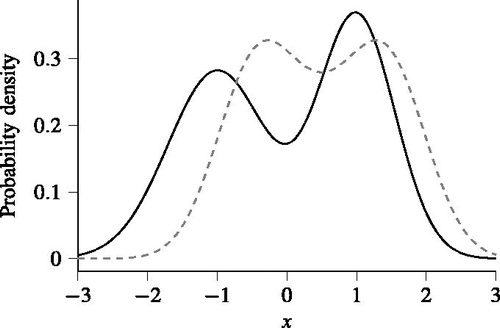
Figure 1 shows the distributions $g\left(\cdot \right)$ (black solid line) and $h\left(\cdot \right)$ (gray dashed line). Both distributions are Gaussian mixtures; that is, both pdfs equal the sum of multiple weighted Gaussian distributions. The pdf $g\left(\cdot \right)$ corresponds to the average of 2 Gaussian distributions with means of $-1$ and $1$ and standard deviations of $0.5$ and $0.3,$ respectively. The pdf $h\left(\cdot \right)$ corresponds to the average of 3 Gaussian distributions with means of $-0.5,$ $0.5,$ and $1.5,$ and standard deviations of $0.3,$ $0.5,$ and $0.3,$ respectively.

Figure 1. The true pdfs $g\left(\cdot \right)$ (black solid line) and $h(\cdot )$ (gray dashed line) that are used to illustrate the quantification of the completeness.

The expectation $\mathrm{E}[\cdot ]$ of Eq. (1)(1) $${\mathrm{MISE}}_{\mathit{f}}\left(n\right)=\mathrm{E}\left[{\int }_{{\mathbb{R}}^{\mathrm{d}}}{\left(f\left(x\right)-\widehat{f}\left(x;n\right)\right)}^2\mathrm{ }\mathrm{d}x\right].$$(1) is estimated by repeating the estimation of the pdf 200 times, such that the real MISE is approximated: (13) $${\mathrm{MISE}}_f\left(n\right)\approx \frac{1}{m}{\sum }_{j=1}^m{\int }_{{\mathbb{R}}^d}{\left(f\left(x\right)-{\widehat{f}}_j\left(x;n\right)\right)}^2\mathrm{ }\mathrm{d}x,$$(13) where ${\widehat{f}}_j(x;n)$ is the $j$th estimate and $m=200.$

All 3 pdfs are estimated using Eq. (2)(2) $$\widehat{f}\left(x;n\right)=\frac{1}{n{h}^d}{\sum }_{i=1}^{n}K\left(\frac{x-X_i}{h}\right).$$(2) . We use leave-one-out cross-validation to compute the bandwidth $h$ (see also Duin 1976) because this minimizes the Kullback-Leibler divergence between the real pdf $f(\cdot )$ and the estimated pdf $\widehat{f}(\cdot ;n)$ (Turlach 1993; Zambom and Dias 2013). Note that although the estimation of the pdfs is repeated 200 times to accurately approximate the MISE using Eq. 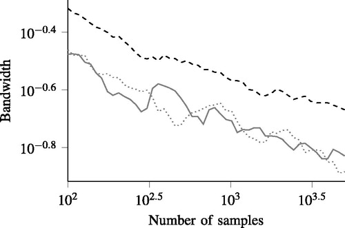(13)(13) $${\mathrm{MISE}}_f\left(n\right)\approx \frac{1}{m}{\sum }_{j=1}^m{\int }_{{\mathbb{R}}^d}{\left(f\left(x\right)-{\widehat{f}}_j\left(x;n\right)\right)}^2\mathrm{ }\mathrm{d}x,$$(13) , the bandwidth is only determined once for a specific number of samples. All of the 199 other times, the same bandwidths are adopted. The resulting bandwidths are shown in Figure 2. The bandwidth of $\widehat{f}(\cdot ;n)$ (black dashed line) is significantly larger than the bandwidths of $\widehat{g}(\cdot ;n)$ (gray solid line) and $\widehat{h}(\cdot ;n)$ (gray dotted line). This result is not surprising: Because $\widehat{f}(\cdot ;n)$ represents a bivariate distribution, it requires more data to have a similar bandwidth compared with a univariate distribution (Scott and Sain 2005).

Figure 2. The bandwidths of $\widehat{f}(\cdot ;n)$ (black dashed line), $\widehat{g}(\cdot ;n)$ (gray solid line), and $\widehat{h}(\cdot ;n)$ (gray dotted line) for the example with artificial data. The bandwidths are computed using leave-one-out cross-validation for different numbers of samples $n.$

Figure 3 shows the results of this example. The black lines show the real MISEs, approximated using Eq. (13)(13) $${\mathrm{MISE}}_f\left(n\right)\approx \frac{1}{m}{\sum }_{j=1}^m{\int }_{{\mathbb{R}}^d}{\left(f\left(x\right)-{\widehat{f}}_j\left(x;n\right)\right)}^2\mathrm{ }\mathrm{d}x,$$(13) , where the black solid line represents the MISE when $f(\cdot )$ is directly estimated and the black dashed line represents the MISE when Eq. (10)(10) $$f\left(x\right)=g\left(y\right)h\left(z\right),$$(10) is used. The MISE is significantly lower when it is correctly assumed that the 2 parameters are independent. One way to look at this is that the degree of freedom of $f\left(\cdot \right)$ is reduced when assuming that the 2 parameters are independent and this lower degree of freedom leads to a more certain estimate. Hence, the MISE is lower.

Figure 3. The real MISEs (black lines) of the example of with the artificial data, approximated using Eq. (13)(13) $${\mathrm{MISE}}_f\left(n\right)\approx \frac{1}{m}{\sum }_{j=1}^m{\int }_{{\mathbb{R}}^d}{\left(f\left(x\right)-{\widehat{f}}_j\left(x;n\right)\right)}^2\mathrm{ }\mathrm{d}x,$$(13) , and the measures that are used to quantify the completeness (gray lines). The solid lines show the result of estimating a bivariate pdf, so here Eq. (8)(8) $$J_f\left(n\right)=\frac{h^4}{4}{\sigma }_K^4{\int }_{{\mathbb{R}}^d}{\left({\nabla }^2\widehat{f}\left(x;n\right)\right)}^2\mathrm{ }\mathrm{d}x+\frac{{\mu }_K}{n{h}^d}.$$(8) is used to quantify the completeness. The dashed lines show the result of estimating 2 univariate pdfs and combining them according to Eq. (10)(10) $$f\left(x\right)=g\left(y\right)h\left(z\right),$$(10) to create a bivariate pdf, so Eq. (12)(12) $$J_f\left(n\right)=J_g\left(n\right){\int }_{{\mathbb{R}}^{d_z}}\widehat{h}{\left(z;n\right)}^2\mathrm{ }\mathrm{d}z+J_h\left(n\right){\int }_{{\mathbb{R}}^{d_y}}\widehat{g}{\left(y;n\right)}^2\mathrm{ }\mathrm{d}y+J_g\left(n\right)\cdot J_h\left(n\right).$$(12) is used to quantify the completeness. The gray areas show the interval $\left[\mu -3\sigma ,\mu +3\sigma \right],$ where $\mu$ and $\sigma$ denote the mean and standard deviation, respectively, of the measures of Eqs. (8)(8) $$J_f\left(n\right)=\frac{h^4}{4}{\sigma }_K^4{\int }_{{\mathbb{R}}^d}{\left({\nabla }^2\widehat{f}\left(x;n\right)\right)}^2\mathrm{ }\mathrm{d}x+\frac{{\mu }_K}{n{h}^d}.$$(8) and (12)(12) $$J_f\left(n\right)=J_g\left(n\right){\int }_{{\mathbb{R}}^{d_z}}\widehat{h}{\left(z;n\right)}^2\mathrm{ }\mathrm{d}z+J_h\left(n\right){\int }_{{\mathbb{R}}^{d_y}}\widehat{g}{\left(y;n\right)}^2\mathrm{ }\mathrm{d}y+J_g\left(n\right)\cdot J_h\left(n\right).$$(12) when repeating the experiment 200 times.

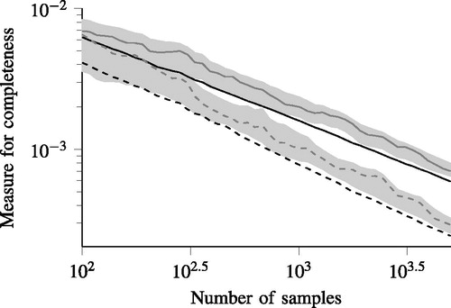
The gray lines in Figure 3 show the measures to quantify the completeness of the data. The gray solid line shows the result of applying Eq. (8)(8) $$J_f\left(n\right)=\frac{h^4}{4}{\sigma }_K^4{\int }_{{\mathbb{R}}^d}{\left({\nabla }^2\widehat{f}\left(x;n\right)\right)}^2\mathrm{ }\mathrm{d}x+\frac{{\mu }_K}{n{h}^d}.$$(8) and the gray dashed line shows the result of applying Eq. (12)(12) $$J_f\left(n\right)=J_g\left(n\right){\int }_{{\mathbb{R}}^{d_z}}\widehat{h}{\left(z;n\right)}^2\mathrm{ }\mathrm{d}z+J_h\left(n\right){\int }_{{\mathbb{R}}^{d_y}}\widehat{g}{\left(y;n\right)}^2\mathrm{ }\mathrm{d}y+J_g\left(n\right)\cdot J_h\left(n\right).$$(12) . Both lines follow the same trend as the black solid line and the black dashed line, respectively. This illustrates that the measures Eqs. (8)(8) $$J_f\left(n\right)=\frac{h^4}{4}{\sigma }_K^4{\int }_{{\mathbb{R}}^d}{\left({\nabla }^2\widehat{f}\left(x;n\right)\right)}^2\mathrm{ }\mathrm{d}x+\frac{{\mu }_K}{n{h}^d}.$$(8) and (12)(12) $$J_f\left(n\right)=J_g\left(n\right){\int }_{{\mathbb{R}}^{d_z}}\widehat{h}{\left(z;n\right)}^2\mathrm{ }\mathrm{d}z+J_h\left(n\right){\int }_{{\mathbb{R}}^{d_y}}\widehat{g}{\left(y;n\right)}^2\mathrm{ }\mathrm{d}y+J_g\left(n\right)\cdot J_h\left(n\right).$$(12) are applicable for estimating the real MISE of Eq. (1)(1) $${\mathrm{MISE}}_{\mathit{f}}\left(n\right)=\mathrm{E}\left[{\int }_{{\mathbb{R}}^{\mathrm{d}}}{\left(f\left(x\right)-\widehat{f}\left(x;n\right)\right)}^2\mathrm{ }\mathrm{d}x\right].$$(1) . To show that this is not a mere coincidence, the gray areas in Figure 3 show the interval $\left[\mu -3\sigma ,\mu +3\sigma \right],$ where $\mu$ and $\sigma$ denote the mean and standard deviation, respectively, of the measures of Eqs. (8)(8) $$J_f\left(n\right)=\frac{h^4}{4}{\sigma }_K^4{\int }_{{\mathbb{R}}^d}{\left({\nabla }^2\widehat{f}\left(x;n\right)\right)}^2\mathrm{ }\mathrm{d}x+\frac{{\mu }_K}{n{h}^d}.$$(8) and (12)(12) $$J_f\left(n\right)=J_g\left(n\right){\int }_{{\mathbb{R}}^{d_z}}\widehat{h}{\left(z;n\right)}^2\mathrm{ }\mathrm{d}z+J_h\left(n\right){\int }_{{\mathbb{R}}^{d_y}}\widehat{g}{\left(y;n\right)}^2\mathrm{ }\mathrm{d}y+J_g\left(n\right)\cdot J_h\left(n\right).$$(12) when repeating the experiment 200 times. Note that the measures of completeness are consistently higher than the real MISE. This can be explained by the fact that the measures of completeness are approximations of the AMISE and the AMISE itself is always higher than the real MISE under some mild conditions; see theorem 4.2 of Marron and Wand (1992).

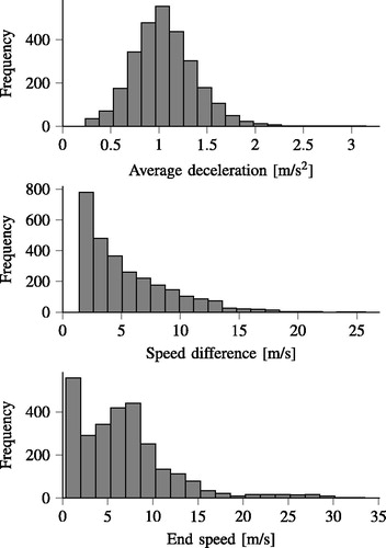
Figure 4. Histogram of the data used for the example with the real data.

Example with real data

In this example, 60 h of naturalistic driving data from 20 different drivers (see also de Gelder and Paardekooper 2017) are used to extract approximately 2,800 braking activities. Three parameters are used to describe each braking activity: The average deceleration, the total speed difference, and the end speed. A histogram of each of these parameters is shown in Figure 4. Note that these braking activities do not include full stops—that is, activities where the end speed is zero—because the distribution of the end speed will have a large peak at zero. The AMISE of Eq. (4)(4) $${\mathrm{AMISE}}_f\left(n\right)=\frac{h^4}{4}{\sigma }_K^4{\int }_{{\mathbb{R}}^d}{\left({\nabla }^{2}f\left(x\right)\right)}^2\mathrm{ }\mathrm{d}x+\frac{{\mu }_K}{n{h}^d}.$$(4) deviates more from the real MISE of Eq. (1)(1) $${\mathrm{MISE}}_{\mathit{f}}\left(n\right)=\mathrm{E}\left[{\int }_{{\mathbb{R}}^{\mathrm{d}}}{\left(f\left(x\right)-\widehat{f}\left(x;n\right)\right)}^2\mathrm{ }\mathrm{d}x\right].$$(1) , especially for larger bandwidths, when such peaks are present in the underlying distribution (Marron and Wand 1992). Because the measure Eq. (8)(8) $$J_f\left(n\right)=\frac{h^4}{4}{\sigma }_K^4{\int }_{{\mathbb{R}}^d}{\left({\nabla }^2\widehat{f}\left(x;n\right)\right)}^2\mathrm{ }\mathrm{d}x+\frac{{\mu }_K}{n{h}^d}.$$(8) we use for quantification of completeness is based on the AMISE of Eq. (4)(4) $${\mathrm{AMISE}}_f\left(n\right)=\frac{h^4}{4}{\sigma }_K^4{\int }_{{\mathbb{R}}^d}{\left({\nabla }^{2}f\left(x\right)\right)}^2\mathrm{ }\mathrm{d}x+\frac{{\mu }_K}{n{h}^d}.$$(4) , we want to avoid these peaks as much as possible. Therefore, the full stops are excluded. Note, however, that the method can be applied separately for the full stops. In fact, the analysis for full stops will be simpler, because a full stop activity can be parameterized using only 2 parameters because the end speed always equals zero.

The 3 parameters are correlated, so this advocates for the use of a multivariate KDE. However, as we have seen in the first example, the higher the dimension, the higher the measure for completeness will generally be, indicating a lower degree of completeness. So there is a trade-off: Assuming that certain parameters are independent results in an error of the estimated pdf but the resulting MISE, and hence the measure of completeness, will be lower. To illustrate this, we estimate the pdf while assuming all parameters to be dependent and we estimate the pdf while assuming that the average deceleration is independent from the other 2 parameters. Note that the correlation between the average deceleration and the other parameters is fairly low, so this justifies this choice. The speed difference and end speed are highly correlated, so we will not assume that these 2 parameters are independent. Before estimating the pdfs, the parameters are translated and rescaled such that each parameter has a sample mean of zero and a sample variance of one. In this example, $\widehat{f}(\cdot ;n)$ denotes the estimated 3D pdf using all 3 parameters, $\widehat{g}(\cdot ;n)$ denotes the estimated univariate pdf of the average deceleration, and $\widehat{h}(\cdot ;n)$ denotes the estimated bivariate pdf of the speed difference and the end speed.

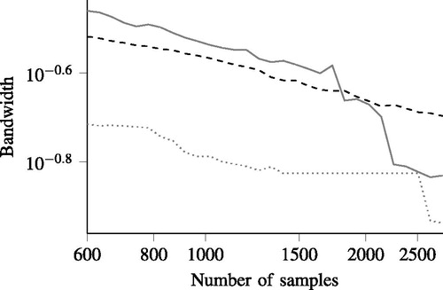
Figure 5 shows the bandwidths of the 3 estimated pdfs for different numbers of samples, starting from $n=600$ samples to approximately $2,800$ samples. As opposed to the bandwidths of our previous example (see Figure 2), the bandwidth of $\widehat{f}(\cdot ;n)$ (black dashed line) is not larger than the bandwidth of $\widehat{g}(\cdot ;n)$ (gray solid line) for low values of $n.$ This is caused by some outliers of the average deceleration, because these outliers have a large influence on the bandwidth of $\widehat{g}(\cdot ;n)$ (Hall 1992). These outliers also influence the bandwidth of $\widehat{f}(\cdot ;n),$ but this influence is less because the bandwidth of $\widehat{f}(\cdot ;n)$ is also influenced by the other parameters.

Figure 5. The bandwidths of $\widehat{f}(\cdot ;n)$ (black dashed line), $\widehat{g}(\cdot ;n)$ (gray solid line), and $\widehat{h}(\cdot ;n)$ (gray dotted line) for the example of with the real data. The bandwidths are computed using leave-one-out cross-validation for different numbers of samples $n.$

The measures of completeness of the data of the braking activities are shown in Figure 6. The solid gray line results from the estimated 3D pdf; that is, $\widehat{f}(\cdot ;n),$ where Eq. (8)(8) $$J_f\left(n\right)=\frac{h^4}{4}{\sigma }_K^4{\int }_{{\mathbb{R}}^d}{\left({\nabla }^2\widehat{f}\left(x;n\right)\right)}^2\mathrm{ }\mathrm{d}x+\frac{{\mu }_K}{n{h}^d}.$$(8) is used to quantify the completeness. The dashed gray line results from the estimated univariate and bivariate pdfs $\widehat{g}(\cdot ;n)$ and $\widehat{h}(\cdot ;n),$ where Eq. (12)(12) $$J_f\left(n\right)=J_g\left(n\right){\int }_{{\mathbb{R}}^{d_z}}\widehat{h}{\left(z;n\right)}^2\mathrm{ }\mathrm{d}z+J_h\left(n\right){\int }_{{\mathbb{R}}^{d_y}}\widehat{g}{\left(y;n\right)}^2\mathrm{ }\mathrm{d}y+J_g\left(n\right)\cdot J_h\left(n\right).$$(12) is used to quantify the completeness. The measure for the completeness is much lower for the latter case, indicating that the uncertainty of the pdf is much lower when it is assumed that the average deceleration is independent of the other 2 parameters.

Figure 6. The measures of completeness for the example with the real data with the assumption that all 3 parameters depend on each other (gray solid line) and with the assumption that the first parameter—that is, the average deceleration—does not depend on the other 2 parameters (gray dashed line). The corresponding black lines represent the least squares logarithmic fits given by Eqs. (14)(14) $$0.019\cdot n^{-0.18},$$(14) and (15)(15) $$0.017\cdot n^{-0.26},$$(15) .

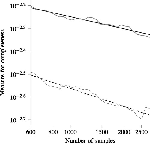
Whether it is better to assume that all parameters are dependent or not depends on the threshold that defines the desired measure and the amount of data. If the threshold is not met, the result can be used to guess how much more data are required by extrapolating the result. To illustrate this, the straight black lines in Figure 6 represent the least squares logarithmic fits of the corresponding gray lines that can be used for extrapolation. These straight solid and dashed black lines are described by the formulas (14) $$0.019\cdot n^{-0.18},$$(14) (15) $$0.017\cdot n^{-0.26},$$(15) respectively. As an example, let us assume that the threshold equals $0.003.$ In that case, $n\approx 800$ would suffice if we assume that the average deceleration is independent from the speed difference and end speed; see the dashed lines in Figure 6 and Eq. (15)(15) $$0.017\cdot n^{-0.26},$$(15) . This threshold, however, is not yet reached when assuming that all parameters are dependent; see the solid lines in Figure 6. Extrapolating the result using Eq. (14)(14) $$0.019\cdot n^{-0.18},$$(14) provides a rough estimate of the required number of samples: $n\approx 28,000;$ that is, 10 times as many samples as we used in this example.

Discussion

Increasing amounts of field data from (naturalistic) driving data are becoming available. The data are used for all kinds of driving-related research, developments, assessments, and evaluations. When deducing claims based on the collected data, we require knowledge about the degree of completeness of the data. We considered the data as a sequence of scenarios, whereas activities are the building blocks of these scenarios. To obtain knowledge about the degree of completeness of the data, we propose a measure to quantify the completeness of the activities. This measure allows us to partially answer questions like “Have we collected enough field data?” We illustrated the method using an artificial data set for which the underlying distributions are known. These results show that the proposed method correctly quantifies the completeness of the activities. We also applied the method on a data set with naturalistic driving to show that the method can be used to estimate the required number of samples.

The measure for quantification of completeness of the set of activities presented in this work is based on the amount of data and the chosen parameterization. More data might be used to achieve a certain threshold. However, it might also be possible to adapt the parameterization to achieve a certain threshold if a parameterization exists that achieves a certain threshold. Hence, the presented method can be used to determine an appropriate parameterization of activities.

The method for quantifying the completeness of a set of activities presented in this work depends on a threshold that needs to be chosen. Only in case of an infinite set of data does the measure for completeness approach zero, so this threshold needs to be larger than zero. This threshold might be different for different applications. For example, when the data are used for determining test scenarios (Elrofai et al. 2018; Ploeg et al. 2018), the desired threshold might be lower than when the data are used for determining driver models (Sadigh et al. 2014; Wang et al. 2017). Furthermore, the threshold depends on the number of parameters for one activity, denoted by $d$ earlier in this method. Based on experience with the data set used in our second example, assuming that the data set is normalized such that the standard deviation equals one, a threshold between 0.01 and 0.001 gives good results. When a threshold of 0.01 is reached, a reasonably reliable pdf can be constructed to analyze nominal driving behavior, whereas a threshold of around 0.001 is required to also accurately analyze the edge cases.

When using our measure for completeness, the following might be considered. As explained in our article, the measure for completeness is based on the AMISE. It is also mentioned that the AMISE only differs from the MISE by higher-order terms under some mild conditions. This requires the real pdf to be smooth; that is, without large spikes (Marron and Wand 1992). Marron and Wand (1992) also state that the AMISE is strictly higher than the MISE under some mild conditions.³ As a result, it is likely that the measure for completeness, which is an approximation of the AMISE, is higher than the MISE. This could lead to an overestimation of the number of required samples.

The measure for completeness proposed in this article can be regarded as an approximation of the MISE of Eq. (1)(1) $${\mathrm{MISE}}_{\mathit{f}}\left(n\right)=\mathrm{E}\left[{\int }_{{\mathbb{R}}^{\mathrm{d}}}{\left(f\left(x\right)-\widehat{f}\left(x;n\right)\right)}^2\mathrm{ }\mathrm{d}x\right].$$(1) . To minimize the MISE, the approximated pdf should be similar to the real pdf. However, it might be that one is not interested in the exact likelihoods of certain values of the parameters but in all possible values that the parameters can have. In this case, one might be interested in the support of the real pdf, because the support of the pdf defines all possible values for which the likelihood is larger than zero; see, for example, Schölkopf et al. (2001).

As mentioned in our problem definition, our problem of quantifying the completeness of a data set can be divided into 3 subproblems. The first subproblem—that is, how to quantify the completeness regarding the scenario classes—can be regarded as the so-called unseen species problem (Bunge and Fitzpatrick 1993; Gandolfi and Sastri 2004) or species estimation problem (Yang et al. 2012). In case of the unseen species problem, the entire population is partitioned into $C$ classes and the objective is to estimate $C$ given only a part of the entire population. To continue the analogy, the second subproblem—that is, how to quantify the completeness regarding all scenarios that fall into a specific scenario class—relates to quantifying whether we have a complete view on the variety among one species, given the number of individuals that we have seen. The third subproblem addresses a part of the scenarios; that is, the activities. In line with the previous analogy, this can be seen as quantifying whether we have a complete view of the parts of the species; for example, its limbs or organs.

Our proposed method answers the third subproblem; that is, how to quantify the completeness regarding the activities. The advantage of using the activities for determining the completeness is that there are only a limited number of types of activities. As a result, for each type of activity, it is expected that there is no need for an extremely large data set to obtain a fair number of similar activities. On the other hand, however, it is not known how much data is required to obtain the desired threshold, because, for example, this depends on the parameterization that is chosen. The next step is to quantify the completeness regarding all scenarios that fall into a specific scenario class. Here, the joint probability of the parameters of different activities in the same scenario class might be considered. Although the presented method can be applied, this might be impractical because the number of parameters will be higher than that for the activities.

In future work, we will extend the method to whole traffic scenarios and scenario classes. Furthermore, we will investigate the appropriate thresholds for the measure to quantify completeness in different applications. The proposed method will be used to evaluate the level of completeness of the data collection aimed at defining relevant test cases for the assessment of automated vehicles.

Acknowledgment

The research leading to this article has been partially realized at the Centre of Excellence for Testing and Research of Autonomous Vehicles at NTU (CETRAN), Singapore.

Notes

1 The pdf $f(\cdot )$ needs to comply with the regularity conditions, $K\left(u\right)\ge 0, \forall u,$ ${\int }_{{\mathbb{R}}^d}K\left(u\right) \mathit{du}=1,$ and ${\sigma }_K$ from Eq. (5) is not infinite.

2 For the sake of brevity, the proof is omitted from this article. The main idea is based on the variance of the product of 2 independent variables (see Goodman 1960) and the assumptions $\mathrm{E}\left[\widehat{g}\left(y;n\right)\right]\approx g\left(y\right)$ for all $y$ and $\mathrm{E}\left[\widehat{h}\left(z;n\right)\right]\approx h\left(z\right)$ for all $z.$

3 The Laplacian of $f\left(\cdot \right)$ needs to be continuous and square-integrable and $K\left(u\right)\ge 0, \forall u.$

References

- Alvarez S, Page Y, Sander U, et al. Prospective effectiveness assessment of ADAS and active safety systems via virtual simulation: a review of the current practices. Paper presented at: 25th International Technical Conference on the Enhanced Safety of Vehicles (ESV); 2017.
- Bashtannyk DM, Hyndman RJ. Bandwidth selection for kernel conditional density estimation. Comput Stat Data Anal. 2001;36:279–298.
- Blair SN, LaMonte MJ, Nichaman MZ. The evolution of physical activity recommendations: how much is enough? Am J Clin Nutr. 2004;79:913S–920S.
- Broggi A, Buzzoni M, Debattisti S, et al. Extensive tests of autonomous driving technologies. IEEE Trans Intell Transp Syst. 2013;14:1403–1415.
- Bunge J, Fitzpatrick M. Estimating the number of species: a review. J Am Stat Assoc. 1993;88:364–373.
- Calonico S, Cattaneo MD, Farrell MH. On the effect of bias estimation on coverage accuracy in nonparametric inference. J Am Stat Assoc. 2018;113:767–779.
- Chen Y-C. A tutorial on kernel density estimation and recent advances. Biostat Epidemiol. 2017;1:161–187.
- Chiu S-T. A comparative review of bandwidth selection for kernel density estimation. Stat Sin. 1996;6:129–145.
- de Gelder E, Paardekooper J-P. Assessment of automated driving systems using real-life scenarios. Paper presented at: IEEE Intelligent Vehicles Symposium (IV); 2017.
- Dingus TA, Guo F, Lee S, et al. Driver crash risk factors and prevalence evaluation using naturalistic driving data. Proc Natl Acad Sci USA. 2016;113:2636–2641.
- Duin. On the choice of smoothing parameters for Parzen estimators of probability density functions. IEEE Trans Comput. 1976;25:1175–1179.
- Elrofai H, Paardekooper J-P, de Gelder E, Kalisvaart S, Op den Camp O. Scenario-Based Safety Validation of Connected and Automated Driving. Helmond, The Netherlands: Netherlands Organization for Applied Scientific Research, TNO; 2018.
- Elrofai H, Worm D, Op den Camp O. Scenario identification for validation of automated driving functions. In: Meyer G, ed. Advanced Microsystems for Automotive Applications 2016. Berlin, Germany: Springer; 2016:153–163.
- Gandolfi A, Sastri CC. Nonparametric estimations about species not observed in a random sample. Milan J Math. 2004;72:81–105.
- Geyer S, Baltzer M, Franz B, et al. Concept and development of a unified ontology for generating test and use-case catalogues for assisted and automated vehicle guidance. IET Intelligent Transport Systems. 2014;8:183–189.
- Goodman LA. On the exact variance of products. J Am Stat Assoc. 1960;55:708–713.
- Guest G, Bunce A, Johnson L. How many interviews are enough? An experiment with data saturation and variability. Field Methods. 2006;18:59–82.
- Hall P. On global properties of variable bandwidth density estimators. Ann Stat. 1992;20:762–778.
- Jones MC, Marron JS, Sheather SJ. A brief survey of bandwidth selection for density estimation. J Am Stat Assoc. 1996;91:401–407.
- Kasper D, Weidl G, Dang T, et al. Object-oriented Bayesian networks for detection of lane change maneuvers. IEEE Intelligent Transportation Systems Magazine. 2012;4:19–31.
- Klauer SG, Dingus TA, Neale VL, Sudweeks JD, Ramsey DJ. The Impact of Driver Inattention on Near-Crash/Crash Risk: An Analysis Using the 100-Car Naturalistic Driving Study Data. Blacksburg, VA: NHTSA; 2006.
- Krajewski R, Bock J, Kloeker L, Eckstein L. The HighD dataset: a drone dataset of naturalistic vehicle trajectories on German highways for validation of highly automated driving systems. Paper presented at: IEEE 21st International Conference on Intelligent Transportations Systems (ITSC); 2018.
- Marks IH, Fong ZV, Stapleton SM, Hung Y-C, Bababekov YJ, Chang DC. How much data are good enough? Using simulation to determine the reliability of estimating POMR for resource-constrained settings. World J Surg. 2018;42:2344–2347.
- Marron JS, Wand MP. Exact mean integrated squared error. Ann Stat. 1992;20:712–736.
- Paardekooper J-P, Montfort S, Manders J, et al. Automatic identification of critical scenarios in a public dataset of 6000 km of public-road driving. Paper presented at: 26th International Technical Conference on the Enhanced Safety of Vehicles (ESV); 2019.
- Parzen E. On estimation of a probability density function and mode. Ann Math Stat. 1962;33:1065–1076.
- Ploeg J, de Gelder E, Slavík M, Querner E, Webster T, de Boer N. Scenario-based safety assessment framework for automated vehicles. Paper presented at: 16th ITS Asia-Pacific Forum; 2018.
- Pütz A, Zlocki A, Bock J, Eckstein L. System validation of highly automated vehicles with a database of relevant traffic scenarios. Paper presented at: 12th ITS European Congress; 2017.
- Rosenblatt M. Remarks on some nonparametric estimates of a density function. Ann Math Stat. 1956;27:832–837.
- Sadigh D, Driggs-Campbell K, Puggelli A, et al. Data-driven probabilistic modeling and verification of human driver behavior. Paper presented at: 2014 AAAI Spring Symposium Series; 2014.
- Schölkopf B, Platt JC, Shawe-Taylor J, Smola AJ, Williamson RC. Estimating the support of a high-dimensional distribution. Neural Comput. 2001;13:1443–1471.
- Scott DW. Multivariate Density Estimation: Theory, Practice, and Visualization. Houston, TX: John Wiley & Sons; 2015.
- Scott DW, Sain SR. Multi-dimensional density estimation. Handbook of Statistics. 2005;24:229–261.
- Silverman BW. Density Estimation for Statistics and Data Analysis. London: CRC Press; 1986.
- Stellet JE, Zofka MR, Schumacher J, Schamm T, Niewels F, Zöllner JM. Testing of advanced driver assistance towards automated driving: a survey and taxonomy on existing approaches and open questions. Paper presented at: IEEE 18th International Conference on Intelligent Transportation Systems; 2015.
- Turlach BA. Bandwidth Selection in Kernel Density Estimation: A Review. Berlin, Germany: Institut für Statistik und Ökonometrie, Humboldt-Universität zu Berlin; 1993.
- Ulbrich S, Menzel T, Reschka A, Schuldt F, Maurer M. Defining and substantiating the terms scene, situation, and scenario for automated driving. Paper presented at: IEEE 18th International Conference on Intelligent Transportation Systems; 2015.
- Wang W, Liu C, Zhao D. How much data are enough? A statistical approach with case study on longitudinal driving behavior. IEEE Transactions on Intelligent Vehicles. 2017;2:85–98.
- Williamson A, Lombardi DA, Folkard S, Stutts J, Courtney TK, Connor JL. The link between fatigue and safety. Accid Anal Prev. 2011;43:498–515.
- Xie J, Hilal AR, Kulić D. Driving maneuver classification: a comparison of feature extraction methods. IEEE Sens J. 2018;18:4777–4784.
- Yang H, Van Dongen BF, Ter Hofstede AH, Wynn MT, Wang J. Estimating Completeness of Event Logs. 2012. BPM Center Report 12. Eindhoven, The Netherlands: Eindhoven University of Technology.
- Zambom AZ, Dias R. A review of kernel density estimation with applications to econometrics. Int Econ Rev. 2013;5:20–42.
- Zofka MR, Kuhnt F, Kohlhaas R, Rist C, Schamm T, Zöllner JM. Data-driven simulation and parametrization of traffic scenarios for the development of advanced driver assistance systems. Paper presented at: 18th International Conference on Information Fusion; 2015.