Where Do Priors Come From? Applying Guidelines to Construct Informative Priors in Small Sample Research

Abstract

This article demonstrates the usefulness of Bayesian estimation with small samples. In Bayesian estimation, prior information can be included, which increases the precision of the posterior distribution. The posterior distribution reflects likely parameter values given the current state of knowledge. An issue that has received little attention, however, is the acquisition of prior information. This study provides general guidelines to collect prior knowledge and formalize it in prior distributions. Moreover, this study demonstrates with an empirical application how prior knowledge can be acquired systematically. The article closes with a discussion that also warns against the misuse of prior information.

Small samples occur regularly in social sciences for various reasons. Sometimes the size of the population is extremely limited, for example in children with a rare disease (Van der Lee, Wesseling, Tanck, & Offringa, 2008), or juvenile females charged with murder (Roe-Sepowitz, 2009). The population can also be difficult to recruit and prone to drop-out because they are homeless, institutionalized, or playing truant (Mäkelä & Huhtanen, 2010; McCabe, Kloska, Veliz, Jager, & Schulenberg, 2016; Peeters, Monshouwer, Janssen, Wiers, & Vollebergh, 2014). Factors such as costs (Rocchetti et al., 2013) and ethical constraints (Van der Lee et al., 2008) may also make efforts to obtain a larger sample quite difficult (or impossible).

One of the consequences of small samples such as those described above is low statistical power (i.e., inflated Type II error, see, e.g. Muthén & Curran, 1997, for a simulation study). Non-significant p values, which likely follow from underpowered analyses, cannot be meaningfully interpreted in the null hypothesis significance testing (NHST) framework. Consequently, researchers often refrain from analyzing interesting (i.e., exceptional) groups and deviate from recommended cut-offs to cover larger groups (e.g., Heron et al., 2013; Scharkow, Festl, & Quandt, 2014) or need to conclude that power was too low to detect the foreseeable small effect (e.g., Mahu, Doucet, O’Leary-Barrett, & Conrod, 2015).

In Bayesian statistics,¹ on the other hand, prior information is combined with the data in the analysis resulting in a posterior distribution that, irrespective of sample size, can be interpreted as a distribution displaying the probability of parameter values. Prior distributions can incorporate information about model parameters that researchers have before seeing the data. Sometimes researchers lack information, but often they are able to limit the admissible parameter space. For example, a prior distribution for a mean could exclude values that are outside the range of the measurement scale. Such a specification already increases the precision of the posterior distribution. Alternatively, a researcher may be able to specify a normal prior distribution that favors some values over others. When no prior information is available, an uninformative prior can be adopted that typically specifies a wide range of parameter values as probable. When a prior distribution becomes narrower because more prior information becomes available, the posterior distribution is affected increasingly by the prior information and becomes narrower and more informative as well. One could state that statistical power ² increases, and inference errors are less likely to occur (see Van de Schoot, Winter, Ryan, Zondervan-Zwijnenburg, & Depaoli, 2017, for an overview of simulation results in the last 25 years). Furthermore, prior distributions can avoid inadmissible estimates and convergence issues in Bayesian estimation. Typical frequentist estimation methods like maximum likelihood (ML) estimation have been shown to suffer from these problems by several simulation studies (e.g., Boomsma & Hoogland, 2001; Hox & Maas, 2001; Meuleman & Billiet, 2009; Tolvanen, 2000). In sum, Bayesian estimation with informative priors results in meaningful output, even with small samples, and can increase the precision of the result when prior information is available. Note however, that even though prior information will increase the precision of the estimates with small samples, we strongly recommend collecting larger samples if this is possible in any way.

The advantages of Bayesian estimation with informative priors for small sample research may be clear, but the current literature does not demonstrate how prior information can be collected systematically, and how priors subsequently should be specified with the obtained information. The current study addresses this gap in the literature. We present guidelines to support researchers that are interested in conducting a Bayesian analysis with informative priors. We, however, do not only present guidelines, we also report on our efforts to actually follow them in the context of an empirical application concerning a latent growth model. For this application, we search for prior information and subsequently formalize the information into prior distributions. The empirical application does not represent the “ideal” situation. On the contrary, the application is a realistic study for which prior information is not easily acquired. With this application, we show what a researcher can do to obtain prior information in complex situations, and what there is left to do, when things do not work out as hoped for. We expect that social scientists who happen to operate under ideal circumstances can easily derive the appropriate steps to take from this example as well. Finally, the paper provides a discussion on how priors should, and should not be used.

GUIDELINES

The following general guidelines can support researchers interested in constructing informative priors for parameters:

• Determine what strategy suits the project of interest best with questions such as:

  • - Could prior information likely be found in the literature (e.g., meta-analyses, reviews, empirical studies)? Note that the quantification of prior information is more straightforward when the literature covers the same variables obtained with the same measures as the data of interest.

  • - Are there experts on the subject matter, and who are they? How can experts contribute? Would experts be able to specify priors for the parameters in the model at hand, or can they contribute in a different manner?

  • - What general knowledge is available about the model parameters?

  • - Is it possible to increase the information in the data by increasing the sample size?

• Determine how to gather the information systematically. Keep a log of every decision (see, e.g., the logbook provided at osf.io/aw8fy) (Zondervan-Zwijnenburg, Peeters, Depaoli, & Van de Schoot, 2017, October).

• When you intend to construct informative priors, visualize them. A visualization (e.g., with R) quickly shows whether the prior specifications that you consider are reasonable.

• When conducting a Bayesian analysis, always provide the following: (1) the origin of and reason behind the priors, and (2) the exact specifications of the priors. See Depaoli and Van de Schoot (2015) for further instructions on reporting Bayesian analyses.

• Conduct a sensitivity analysis and show the impact of various priors on the posterior estimates (Van de Schoot et al., 2017). Consider at least the derived informative priors and default priors, but conservative or skeptical priors may be interesting to examine as well.

• Try to understand and interpret differences between analyses with different priors.

EMPIRICAL APPLICATION

To demonstrate how prior information can be systematically collected and included in a Bayesian analysis, we compared the development rate of cognitive performance in young heavy cannabis users to that of their nonusing peers in a two-group latent growth model (LGM). We did so in a high-risk sample of young adolescents enrolled in special education because of behavioral problems (Peeters et al., 2014). Young was defined as younger than age 15, because cannabis use before age 15 is considered as early onset (Jacobus, Bava, Cohen-Zion, Mahmood, & Tapert, 2009). A relation between cannabis use and poorer attention, learning, and processing speed is expected especially with early onset of use (Fontes et al., 2011; Jacobus et al., 2009; Schweinsburg, Brown, & Tapert, 2008). By using a high-risk sample, the heavy cannabis users and their nonusing peers are better comparable. However, this also limits the total sample size. In addition, heavy cannabis-using adolescents were expected to be a minority even in this sample. Thus we have a small and unbalanced samples, for which several simulations studies have demonstrated that ML estimation results in low power, and computational issues (e.g., Hox & Maas, 2001; Meuleman & Billiet, 2009; Muthén & Curran, 1997).

In Bayesian estimation informative priors can increase the precision of the posterior outcome, and even when the statistical power would be low, the posterior distribution would still be meaningful and easy to interpret. From the posterior distribution, a measure of central tendency (e.g., the mean, median, or mode) is usually taken to reflect a point estimate for the parameter of interest. Additionally, a 95% credibility interval can be derived from the posterior distribution. This interval has a 95% chance of containing the true parameter value, given the data and the prior. The frequentist 95% confidence interval, in contrast, cannot be interpreted as an interval that has a 95% chance of containing the true value. The confidence interval only contains the true population value in 95% of the intervals over a long run of trials. Thus, the Bayesian framework provides solutions that are more meaningful. Additionally, prior distributions can prevent inadmissible solutions by assigning zero probability to ranges of values that the parameter cannot take (e.g., negative values for variances). All in all, we had various reasons to conduct a Bayesian analysis and search for prior information.

METHOD

Participants

The original study of Peeters et al. (2014) concerned 374 adolescents (330 boys, 44 girls) who attended special education schools for youth with externalizing behavioral problems in The Netherlands. From this group, adolescents younger than age 15 at the first assessment were selected to ensure that cannabis use at the first wave reflected an early onset. Twenty-eight participants did not indicate their age in years at the first wave. To avoid a loss of power, missing data for age was imputed by means of the R-package mice (Van Buuren & Groothuis-Oudshoorn, 2011).

Participants’ ages could be easily imputed, because age in full years was assessed repeatedly in the 2 years that assessments were taken. Exact birth dates, however, were not available. The mean age over 10 imputations for each participant was computed. Participants with a rounded mean age younger than 15 were selected for further analyses (n = 331).

Subsequently, we mimicked previous literature (Mahmood, Jacobus, Bava, Scarlett, & Tapert, 2010) in that nonusers and heavy users were selected to contrast the two extremes. Students were selected based on their response to the question: “How often have you used cannabis during the past 6 months?”. The five answer categories to this question were 1 (I have not used cannabis/marijuana), 2 (Once a month), 3 (2–4 times a month), 4 (2–3 times a week), and 5 (4 times a week or more). Adolescents who selected the first answer category “I have not used cannabis/marijuana” were identified as nonusers (n = 252, mean age = 13.30, 90.4% male). All adolescents who selected the fourth and fifth answer category (n = 16, mean age = 13.38, 81.3% male) met the requirements to be considered heavy cannabis users (Barnes, Barnes, & Patton, 2005). The 25 and 13 participants that selected Category 2 and 3, respectively, were not included, as well as the 25 participants that chose not to answer this question.

Measures

Working Memory

Working memory performance was selected as a measure of cognitive performance because working memory continues to develop throughout adolescence (Best & Miller, 2010). Working memory performance was assessed with the nonverbal self-ordered pointing task (SOPT) with representational drawings of everyday objects (Petrides & Milner, 1982). In this task, participants were instructed to select a different picture out of a set of pictures each time, while after each choice the location of the pictures changed and they were not allowed to select the same location consecutively. The task included one practice trial with a set of four unique pictures, and four assessment trials with sets of 6, 8, 10, and 12 unique pictures. The percentage of correct choices on the task was used as an indication of working memory performance. Details of the assessment can be found in Peeters et al. (2014). In the current data set, working memory performance was assessed four times over 2 years with intervals of approximately 6 months (Peeters et al., 2014).

Alcohol Use

We corrected the development of both groups for the impact of quantity and frequency of alcohol use at the start of the study, as recommended by Jacobus et al. (2009). Alcohol use was assessed by means of a quantity frequency measure (QF). The QF was a multiplication of the number of days a week that the adolescent usually consumed alcohol with the number of glasses that were usually consumed on drinking days. A detailed description can be found in Peeters et al. (2014).

Statistical Approach

To investigate the difference in cognitive development between heavy cannabis users and nonusers, the latent growth model as shown in Figure 1 was the preferred analysis. The repeated measures (i.e., , , , and ) were represented by the four assessments of SOPT scores, and the covariate for this model was a measure of alcohol use quantity and frequency at the start of the study (i.e.,). The quadratic slope was included because the linear increase in the percentage of correct responses on the task was expected to level off over time. Because this effect was expected to be similar for both groups, the quadratic slope was constrained equal over groups accordingly. The linear growth factor in this model represents the linear growth rate at the first time point while a quadratic factor is modeled. As indicated above, the model has one covariate representing an observed time-invariant predictor. As a result the latent time variables technically have intercepts instead of means. However, to avoid confusion between the intercept growth factor and the intercepts of the latent growth factors, the latter will be referred to as means throughout the article. To assess the growth rate difference between groups, a new parameter (denoted by ) was constructed by subtracting the linear slope mean of the frequent users group (i.e., the exceptional group) from that of the nonusers group (i.e., the reference group).

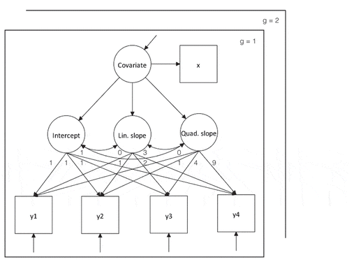
FIGURE 1 Multiple group latent growth model with one covariate and groups indicated by . , , , represent four assessments of a developing construct with residual error variances. is a time-invariant predictor of growth that represents the latent variable Covariate without measurement error. The regressions of the latent growth factors , , and Quad. slope on the Covariate are equal over groups.

Prior Knowledge

Prior distributions need to be specified for all parameters in a Bayesian model, but we focused on finding prior knowledge for our main parameters: , and the latent growth means. For the remaining parameters, we used the default settings of Mplus 7.3, that is: for mean of the covariate and for the regression coefficients, for the residual variances and the variance of the covariate, and for the variance-covariance matrix of the growth factors (Muthén & Muthén, 1998-2012). Note that default settings can cause problematic results. See, for instance, Van de Schoot, Broere, Perryck, Zondervan-Zwijnenburg, and Van Loey (2015). We report a sensitivity analysis with varying prior distributions for the remaining parameters in our logbook, which is provided at osf.io/aw8fy (Zondervan-Zwijnenburg et al., 2017, October).

Prior knowledge can be extracted from several resources such as meta analyses, reviews, empirical studies, and experts (O’Hagan et al., 2006). We evaluated potential sources of prior information one by one, and after consideration of each source, it was reevaluated what the next step would be.

Meta-Analyses

A literature search was conducted in Scopus for meta analyses published between January 2000 and December 2013 based on the terms: cannabis, marijuana, adolescent, and cognitive. The search yielded six results. However, none of them were relevant because they concerned nonhealthy subjects (i.e., suffering from psychosis, or schizophrenia; n = 3), and interventions (n = 3), instead of the relation between cannabis use and cognitive impairment (see Zondervan-Zwijnenburg et al., 2017, October, osf.io/aw8fy for references). As a result, the search for prior information had to be continued with respect to the next source of prior information.

Reviews

A search for reviews with the same keywords as for meta analyses yielded 33 English matches. We had to exclude 27 of these studies, because they concerned preventions and interventions (n = 11), schizophrenia and substance use disorders (n = 4), prenatal exposure (n = 5), or did not focus on cognitive effects of cannabis use (n = 7). Consequently, six reviews were considered relevant. Three additional relevant reviews were identified through other resources. The resulting nine reviews were all published in 2008 and 2009 and covered information from 36 articles, including human and animal (preclinical) studies. By analyzing key sentences from the reviews, we learned that a zero effect size for should receive more than zero probability from the priors (see Zondervan-Zwijnenburg et al., 2017, October, osf.io/aw8fy for references and details). Quantitative information about the exact values of the intercept, linear, and quadratic slopes, however, lacked. To find this information with which priors can be constructed, we decided to continue with a search for actual SOPT scores in empirical articles.

Empirical Studies

Because it is not common to mention an assessment instrument in the title, abstract, or keywords of an article, a search engine that evaluates the content of complete articles had to be used. A suitable search engine for this purpose is Google Scholar. In Google Scholar, we used the following search query: self-ordered pointing, child OR adolescent. The search yielded 693 hits. To obtain the most relevant results for our research population, several inclusion criteria were applied. First, actual scores of the SOPT with familiar objects had to be provided in the study. Second, the mean age of the samples studied had to be between 9.5 and 17.5 years, this age range covers the age of the research population 4 years. Third, the version of the SOPT had to include concrete pictures because other versions differ in difficulty, and thus in their scores. Fourth, samples had to consider typically developing children, or children with attention-deficit/hyperactivity disorder (ADHD), oppositional defiant disorder (ODD), and/or conduct disorder (CD). ADHD, ODD, and CD are disorders commonly encountered in special education classes such as those included in the current study. Fifth, studies had to cover samples that were not already covered in (1) previous articles that met the inclusion criteria or (2) the current study.

After correspondence with authors about task and sample ambiguities, 13 out of 693 articles yielded useful information. All obtained SOPT scores were transformed into a percentage of correct responses. An overview of the articles with encountered SOPT scores for children and adolescents is given at osf.io/aw8fy (Zondervan-Zwijnenburg et al., 2017, October). To ensure that the obtained scores were relevant for our specific high-risk sample, we involved experts.

Experts

Two experts were recruited to participate in the current study: A developmental psychopathology professor and a clinician at a secondary school for youth with externalizing behavioral problems. In separate face-to-face meetings, the experts received a questionnaire consisting of an explanatory text and a table. Based on sample descriptions from the selected empirical studies, the experts rated the relevance of these samples for the population of youth with behavioral problems in general and estimated the percentage of cannabis users in the described sample. During the procedure, the experts did not get information on the SOPT scores in the study, nor did they get information about the authors of the study. The intraclass correlation coefficient with respect to the absolute agreement of the two experts about study representativeness was .87, indicating good interrater reliability.

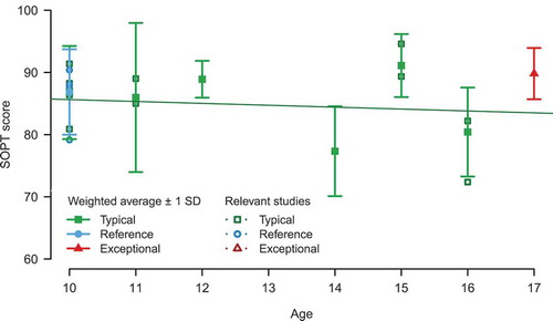
The relevance of the samples rated by both experts was averaged. When the average judgment of sample relevance was higher than .5, the sample relevance was multiplied with the sample size, resulting in a number that was interpreted as the relevant sample size. Based on the relevant sample sizes, a weighted average of the SOPT scores for each age group was computed. Relevant samples with an estimated percentage of cannabis users higher than 50% were considered relevant for the exceptional group.

Figure 2 shows the weighted averages by age and population. As can be seen, only one sample qualified as representative for the exceptional population of heavy cannabis-using youth with externalizing behavioral problems according to the experts. Four samples were considered relevant for the reference group. However, these studies all covered 10-year-olds, yielding only one datapoint from a longitudinal perspective. To construct a prior for the intercept factor at age 13 and the linear slope factor, prior information had to be obtained for at least two age groups. Because these were not available for the population of interest, general knowledge needed to complement the information that we had acquired so far.

FIGURE 2 Weighted self-ordered pointing task scores by age.

General Knowledge and Prior Specification

Intercept

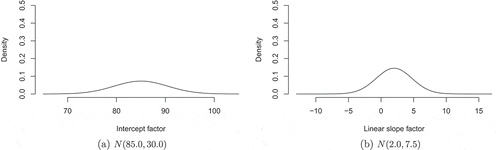
The information on typically developing children indicated that around age 13.5 values between 75 and 95 are most likely. Hence, the prior mean was set at the mean of those values: 85. To determine the variance for this mean, prior mean variances were visualized (see Figure 3a) and the preference of the distribution for some values over others was calculated. With respect to the intercept factor, a variance of 30 implied that values between 80 and 90 were 1.06 times as likely in the prior distribution as values between 90 and 100 (or between 70 and 80), and 1.25 times as likely as values between 100 and 110 (or between 60 and 70). These ratios in the likelihood of values in the prior distribution were considered reasonable, and thus implemented as such.

FIGURE 3 Visualizations of the prior distributions for the latent growth factor means.

Linear Slope

To acquire an idea about the trend over time, a linear regression was fitted to the SOPT scores for typically developing children. The result is represented by the slope in Figure 2. The negative trend, however, is not in line with validated theory (Best & Miller, 2010). In addition, the SOPT scores of typically developing children seemed inconsistent over time. Based on theory, we expected a positive development of SOPT scores over time (Best & Miller, 2010). This expectation was confirmed by the empirical study of Clarke (2009), who found a significant positive cross-sectional correlation of medium size between age and performance on the SOPT for children with ADHD, who were at risk for CD. However, because the prior information derived from the SOPT scores for typically developing children indicated a negative trend, negative values were not excluded. More specifically, given an intercept prior mean of 85, the linear growth mean could be up to 1.75 points per 6 months to reach a score of 95.5 at age 17. However, we expected that the growth rate decreased when higher scores were achieved. Thus, a negative quadratic factor was anticipated, which allowed for a higher linear growth factor. Given the expectation of a negative quadratic factor mean, the linear slope prior mean was set at 2.00 points per 6 months with a prior variance of 7.5. This prior variances caused values between 0 and 4 to be 1.15 times as likely in the prior distribution as values between 4 and 8 (or between 0 and −4). See Figure 3b for a visualization.³

Quadratic Slope

As mentioned, a diminishing growth rate over time can be represented by a negative quadratic growth factor. In the current empirical application, however, a large negative quadratic growth factor might cause a decrease in working memory within the range of the model, whereas this is not expected during adolescence (Best & Miller, 2010). Therefore, the prior mean for the quadratic growth factor was set at −0.1 with a variance of 7.5. The variance of 7.5 is relatively wide for this quadratic slope that we expect to be small. With this variance we reflect that we do not have very specific information for the quadratic slope factor. This distribution has the same shape as that in 0 but is shifted 2.1 points to the left. The combination of the specified priors for the latent growth factor means presupposed an increase of 5.1 in the percentage of correct SOPT entries over the 2 years in which data was collected.

All in all, the final prior distributions were:

(1)

(2)

(3)

Note that we specified normal distributions in all cases, but that other distributional forms (e.g., beta, Cauchy, skewed normal, etc.) can also be considered. Novice appliers of Bayesian statistics might need to be aware of software limitations in this respect. See Depaoli and Van de Schoot (2015) for detailed guidelines on specifying prior distributions.

RESULTS

A Bayesian analysis was conducted in Mplus 7.3 with four chains, a minimum of 50,000 iterations, and BCONVERGENCE was set at an extra strict number of .005. BCONVERGENCE affects the pursued Gelman-Rubin potential scale reduction (PSR; Gelman & Rubin, 1992) criterion value for the model to be considered converged (Muthén & Muthén, 1998-2012). Convergence was obtained at 50.000 iterations. Subsequently, the first half of the iterations was discarded as a burn-in phase. The maximum PSR among the iterations that contributed to the posterior results (i.e., 25.000–50.000) was 1.014. The median of the posterior distribution was interpreted as the point estimate. Traceplots for all parameters showed that the chains had stable means and variances. (See Zondervan-Zwijnenburg et al., 2017, October, osf.io/aw8fy for the data, syntax, and output).

The results of the analysis are provided in Table 1. The 95% (highest posterior density) interval for Δα = [0.17, 7.30](see also Figure 4). The median of this distribution is 3.77. Based on this distribution we can state that we are 98.0% sure that Δα > 0. Thus, young adolescents not using cannabis seem to have a higher working memory increase than their heavy cannabis using peers. Cohen’s d at the median of this distribution is 0.54.

TABLE 1 Main Posterior Parameter Estimates for the Analysis with Informative and Default Priors

	Informative priors			Default priors			Difference
Parameter	M	95%CI		M	95%CI		%
Interceptnonusers	74.00	[72.47, 75.55]		73.22	[71.58, 74.83]		1.07
Interceptusers	78.68	[73.06, 84.20]		75.16	[68.18, 82.30]		4.68
Lienar slopenonusers	6.10	[3.94, 8.26]		7.40	[4.95, 9.95]		–17.68
Linear slopeusers	2.34	[–1.28, 5.96]		4.83	[–0.35, 10.00]		–51.53
Quadratic slope	–1.58	[–2.27, -0.92]		–1.94	[–2.72, –1.18]		18.48
∆α	3.77	[0.17, 7.30]		2.57	[–2.05, 7.28]		46.48

Note. nnonusers = 252, nusers = 16. CI = credibility interval.

FIGURE 4 Samples from the posterior distributions for based on informative priors (darkgrey) and default priors (transparant). Vertical lines indicate the limits of the associated 95% highest posterior density interval.

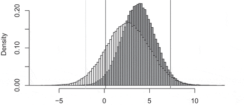
To evaluate the impact of the informative priors on this result, a sensitivity analysis was conducted, which is presented in detail at osf.io/aw8fy (Zondervan-Zwijnenburg et al., 2017, October). The main results for the analysis with default priors are presented in Table 1. The 95% credibility intervals for all parameters in the analysis with informative priors were smaller than the analysis with default priors, indicating that the prior information increased the precision of the final results. The last column shows the relative difference in posterior medians between both analyses. In absolute terms, the discrepancies ranged from 1.07% for the nonusers’ intercept to 51.53% for the heavy users’ linear slope mean. The relative difference between the analyses for Δα was 46.48%. In the analysis with default priors, the 95% interval was Δα = [–2.05, 7.28]with 2.57 as its median (Cohen’s d = .35). 86.4% of the posterior distribution for Δα is larger than 0, and 68.4% is in line with at least a small effect size (i.e., Cohen’s d ≥ .20). The posterior distributions for Δα obtained from the analysis with informative priors and the analysis with default priors are depicted in Figure 4. The figure shows that relative to the posterior from the analysis with informative priors, the posterior from the analysis with default priors is wider and puts a higher probability on lower values for Δα.

CONCLUSION EMPIRICAL APPLICATION

Despite the expected lack of statistical power, the analysis did show that young adolescents not using cannabis most presumably have a stronger working memory growth rate than their heavy cannabis-using peers. Note that we cannot draw causal conclusions, because there may be more differences between the sample of heavy cannabis users and nonusers that relate to their working memory development rate than cannabis alone, even after controlling for quantity and frequency of alcohol use at the start of the study. Furthermore, the information from the data for both groups was substantiated with more general prior information. This general information affected the posterior distribution for the heavy cannabis users more because the sample for this group was smaller and the data thus contained less information. The sensitivity analysis showed that with default priors we would also conclude that we expect that young adolescents not using cannabis most presumably have a stronger working memory growth rate than their heavy cannabis-using peers, but we are less confident. Future studies can use our posterior results, either with informative or default priors, as prior information again. By reporting the exact prior distributions and how they came into being, everyone can review our prior information. By reporting an analysis with uninformative priors as well, we provide a similar insight into data.

DISCUSSION

The aim of the current study was to provide guidance on and to demonstrate how prior information can be collected systematically and subsequently formalized, because this information is lacking in current literature. In the pursuit of this aim, we provided guidelines and demonstrated their application with an empirical application. In the following paragraphs we discuss advantages and disadvantages of different prior information sources, we discuss directions for future research, we discuss the ethical use of Bayes, and end with some concluding thoughts relating back to NHST.

When prior information is scarce, it seems promising to collaborate closely with experts. In the current study, experts contributed to the evaluation of information obtained from other studies. Another option is to let experts determine the prior for the parameter of interest themselves. In that case, the researcher must ensure that the experts understand the parameter of interest, use appropriate heuristics, and avoid fallacies (see also O’Hagan et al., 2006). Under these conditions, collaborating with experts can always increase the precision of the result, in contrast to searching for literature, which may not result in useful prior information. Additionally, published studies may suffer from publication bias. It is important to realize however, that “academic” experts may be affected by this publication bias as well. Furthermore, a procedure to elicit priors for the specific model parameter adjusted to the experts at hand may be nonexistent. Developing a valid and reliable procedure to elicit prior information may be a full research project in itself (see, e.g., Johnson et al., 2010; Zondervan-Zwijnenburg, Van de Schoot-Hubeek, Lek, Hoijtink, & Van de Schoot, 2017), whereas a search for prior information in the literature may resemble an extended systematic literature study that researchers would also conduct to write the introduction to their article. Currently, experts in the social sciences mainly contribute to clinical studies by estimating (success) probabilities (Spiegelhalter, Myles, Jones, & Abrams, 2000). Empirical research on the elicitation of more complex parameters within the social sciences is warranted (O’Hagan et al., 2006).

As was also apparent in the empirical application, prior information does not only affect standard errors, it can also change estimates in case of a discrepancy between the prior information and the data. In the analysis with informative priors, the posterior results in the exceptional group were affected more by the prior distributions than the posterior results of the reference group. The reference group posterior distributions were mainly affected by the data.

Additional research is required with respect to the inclusion of prior information. More specifically, the area of research about the inclusion of highly informative prior distributions is still in its early stages. Researchers may want to test whether a mismatch between the prior and data exists. Methods for such a test need to be further developed to be applicable for applied researchers with all sorts of models. Additionally, some of the reviews discussed in the empirical application considered information from animal studies, but how well can this information serve as prior information in social and behavioral sciences research, should it be merged with prior information from studies on humans, and if so how?

(Un)ethical Use of Bayesian Estimation

Like frequentist NHST, Bayesian estimation methods can be misused. Misuse of Bayesian estimation with informative priors would be to repeatedly conduct analyses with varying priors and only report the analysis with “desirable” results. This is unethical behavior, comparable to “p-hacking” and data fabrication. Instead, researchers should be transparant about the actions and reasoning that led to the priors at hand. In the current study, for example, we conducted a systematic search, reported this search, and provided justifications for the final prior choices. In this manner, readers can decide for themselves whether they are convinced by the information.

A simulation study can clarify how specific prior information should be to obtain posterior results that can convincingly exclude specific parameter values like zero. This may be helpful in designing the search for prior information. However, if the results show that zero will be a likely value a posteriori, researchers should be able to accept this as a conclusion. In studies that are conducted properly, such results should be regarded publication worthy. Irrespective of the results, any publication can provide prior information for future studies on the same topic. In this manner, cumulative science through Bayesian updating is promoted.

Additionally, to promote transparency we advise to demonstrate the impact of other priors on the results by means of a sensitivity analysis (Van Erp, Mulder, & Oberski, conditionally accepted). The sensitivity analysis should be clearly documented as well (see, for example, the logbook provided at osf.io/aw8fy) (Zondervan-Zwijnenburg et al., 2017, October). Clear reporting and sensitivity analyses contribute to transparency, and thus integrity, that is recognized to be important for the survival of social science research (Cumming, 2014). Depaoli & Van de Schoot (2015) developed a 10-point checklist to improve transparency and replication in Bayesian research.

CONCLUDING THOUGHTS

The issues with NHST have been widely discussed (e.g., Cohen, 1994; Cumming, 2014; Kline, 2004; Rozeboom, 1960), and the Bayesian framework offers a viable alternative to this hypothesis testing framework because it can prevent researchers from having to make an oversimplified decision of whether a hypothesis is to be rejected. Bayesian estimation is a beneficial tool that is less restrictive than the conventional NHST framework. It is our hope that this demonstration of how informed priors can be acquired and implemented will aid in broadening the methods typically used for assessing hypotheses in the conventional framework.

The current study showed how prior information can be obtained systematically, and how this information can be formalized into prior distributions. Once again we want to emphasize that specifying highly informative prior distributions is not to be used to achieve statistically significant results. Instead, prior specifications should be used because including available information can be the key to answering questions about populations that otherwise remain unanswered. The search for prior information may be intensive and time consuming, yet it can be rewarding because it provides great insight in the current state of the field, it can improve the analysis, and it results in an update of knowledge.

FUNDING

This work was supported by the Nederlandse Organisatie voor Wetenschappelijk Onderzoek [NWO VIDI 452-14-006];Nederlandse Organisatie voor Wetenschappelijk Onderzoek (NL) [NWO Gravitation 024-001-003].

Additional information

Funding

This work was supported by the Nederlandse Organisatie voor Wetenschappelijk Onderzoek [NWO VIDI 452-14-006];Nederlandse Organisatie voor Wetenschappelijk Onderzoek (NL) [NWO Gravitation 024-001-003]

Notes

¹ To readers interested in a gentle introduction into Bayesian statistics for social scientists, we recommend Kruschke (2014), and Van de Schoot et al. (2013).

² The term power originates from the frequentist setting, where only frequency probabilities can be considered. A frequency probability refers to the expected relative frequency of an outcome given repeated events. Power is the frequency probability of rejecting the null, given that the alternative hypothesis is true. In the Bayesian setting, usually subjective probabilities reflecting a degree of belief are considered, but a subjective probability can be translated to a frequency probability (Press, 2009). For example, a probability of .5 of getting heads from a coin flip can be translated to 5 expected heads in 10 tosses. Hence, one can imagine that a construct like power can be used in the Bayesian context as well (see also Rubin (1984)).

³ No prior was assigned directly to , since this parameter is derived from the linear slope means. To implement a difference between groups with a small effect size, as was indicated by the reviews, information about the residual variance in the linear slope after prediction by the amount of alcohol use was necessary. This information could not be derived from any of the evaluated literature.

REFERENCES

- Barnes, G. E., Barnes, M. D., & Patton, D. (2005). Prevalence and predictors of “heavy” marijuana use in a Canadian youth sample. Substance Use and Misuse, 40(12), 1849–1863. doi:10.1080/10826080500318558
- Best, J. R., & Miller, P. H. (2010). A developmental perspective on executive function. Child Development, 81(6), 1641–1660. doi:10.1111/j.1467-8624.2010.01499.x
- Boomsma, A., & Hoogland, J. J. (2001). The robustness of LISREL modeling revisited. In R. Cudeck, K. G. Jöreskog, & D. Sörbom (Eds.), Structural equation models: Present and future. A festschrift in honor of Karl Jöreskog (pp. 139–168). Lincolnwood, IL: Scientific Software International.
- Clarke, T. L. (2009). Executive functions and overt/covert patterns of conduct disorder symptoms in children with ADHD ( Unpublished doctoral dissertation). University of Maryland.
- Cohen, J. (1994). The earth is round (p < .05). American Psychologist, 49(12), 997–1003. doi:10.1037/0003-066X.49.12.997
- Cumming, G. (2014). The new statistics: Why and how. Psychological Science, 25(1), 7–29. doi:10.1177/0956797613504966
- Depaoli, S., & Van de Schoot, R. (2017). Improving transparency and replication in Bayesian statistics: The WAMBS-Checklist. Psychological Methods, 22(2), 240. doi:10.1037/met0000065
- Fontes, M., Bolla, K., Cunha, P., Almeida, P., Jungerman, F., Laranjeira, R., … Lacerda, A. (2011). Cannabis use before age 15 and subsequent executive functioning. British Journal of Psychiatry, 198, 442–447. doi:10.1192/bjp.bp.110.077479
- Gelman, A., & Rubin, D. B. (1992). Inference from iterative simulation using multiple sequences. Statistical Science, 7, 457–472. doi:10.1214/ss/1177011136
- Heron, J., Barker, E. D., Joinson, C., Lewis, G., Hickman, M., Munafò, M., & Macleod, J. (2013). Childhood conduct disorder trajectories, prior risk factors and cannabis use at age 16: Birth cohort study. Addiction, 108(12), 2129–2138. doi:10.1111/add.12268
- Hox, J., & Maas, C. J. (2001). The accuracy of multilevel structural equation modeling with pseudobalanced groups and small samples. Structural Equation Modeling, 8(2), 157–174. doi:10.1207/S15328007SEM08021
- Jacobus, J., Bava, S., Cohen-Zion, M., Mahmood, O., & Tapert, S. (2009). Functional consequences of marijuana use in adolescents. Pharmacology, Biochemistry and Behavior, 4, 559–565. doi:10.1016/j.pbb.2009.04.001
- Johnson, S. R., Tomlinson, G. A., Hawker, G. A., Granton, J. T., Grosbein, H. A., & Feldman, B. M. (2010, April). A valid and reliable belief elicitation method for Bayesian priors. Journal of Clinical Epidemiology, 63(4), 370–383. doi:10.1016/j.jclinepi.2009.08.005
- Kline, R. B. (2004). Beyond significance testing: Reforming data analysis methods in behavioral research. Washington, DC, USA: American Psychological Association.
- Kruschke, J. K. (2014). Doing Bayesian data analysis: A tutorial with R, JAGS, and Stan (2nd ed.). San Diego, CA: Academic Press.
- Mahmood, O. M., Jacobus, J., Bava, S., Scarlett, A., & Tapert, S. F. (2010). Learning and memory performances in adolescent users of alcohol and marijuana: Interactive effects. Journal of Studies on Alcohol and Drugs, 71(6), 885–894. doi:10.15288/jsad.2010.71.885
- Mahu, I. T., Doucet, C., O’Leary-Barrett, M., & Conrod, P. J. (2015). Can cannabis use be prevented by targeting personality risk in schools? Twenty-four-month outcome of the adventure trial on cannabis use: A cluster-randomized controlled trial. Addiction, 110(10), 1625–1633. doi:10.1111/add.12991
- Mäkelä, P., & Huhtanen, P. (2010). The effect of survey sampling frame on coverage: The level of and changes in alcohol-related mortality in Finland as a test case. Addiction, 105(11), 1935–1941. doi:10.1111/j.1360-0443.2010.03069.x
- McCabe, S. E., Kloska, D. D., Veliz, P., Jager, J., & Schulenberg, J. E. (2016). Developmental course of nonmedical use of prescription drugs from adolescence to adulthood in the united states: National longitudinal data. Addiction, 111(12), 2166–2176. doi:10.1111/add.13504
- Meuleman, B., & Billiet, J. (2009). A Monte Carlo sample size study: How many countries are needed for accurate multilevel SEM? Survey Research Methods, 3, 45–58.
- Muthén, B. O., & Curran, P. J. (1997). General longitudinal modeling of individual differences in experimental designs: A latent variable framework for analysis and power estimation. Psychological Methods, 2, 371–402. doi:10.1037/1082-989X.2.4.371
- Muthén, L. K., & Muthén, B. O. (1998-2012). Mplus user’s guide (7th ed.). Los Angeles, CA: Muthén & Muthén.
- O’Hagan, A., Buck, C. E., Daneshkhah, A., Eiser, J. R., Garthwaite, P. H., Jenkinson, D. J., … Rakow, T. (2006). Uncertain judgements: Eliciting experts’ probabilities. Chichester, England: John Wiley & Sons. doi:10.1002/0470033312
- Peeters, M., Monshouwer, K., Janssen, T., Wiers, R. W., & Vollebergh, W. A. (2014). Working memory and alcohol use in at-risk adolescents: A 2-year follow-up. Alcoholism: Clinical and Experimental Research, 38(4), 1176–1183. doi:10.1111/acer.12339
- Petrides, M., & Milner, B. (1982). Deficits on subject-ordered tasks after frontal- and temporal-lobe lesions in man. Neuropsychologia, 20, 249–262. doi:10.1016/0028-3932(82)90100-2
- Press, S. J. (2009). Subjective and objective Bayesian statistics: Principles, models, and applications (Vol. 590). Hoboken, NJ, USA: John Wiley & Sons.
- Rocchetti, M., Crescini, A., Borgwardt, S., Caverzasi, E., Politi, P., Atakan, Z., & Fusar-Poli, P. (2013). Is cannabis neurotoxic for the healthy brain? A meta-analytical review of structural brain alterations in non-psychotic users. Psychiatry and Clinical Neurosciences, 67(7), 483–492. doi:10.1111/pcn.12085
- Roe-Sepowitz, D. E. (2009). Comparing male and female juveniles charged with homicide child maltreatment, substance abuse, and crime details. Journal of Interpersonal Violence, 24(4), 601–617. doi:10.1177/0886260508317201
- Rozeboom, W. W. (1960). The fallacy of the null-hypothesis significance test. Psychological Bulletin, 57(5), 416–428. doi:10.1037/h0042040
- Rubin, D. B. (1984). Bayesianly justifiable and relevant frequency calculations for the applied statistician. The Annals of Statistics, 12(4), 1151–1172. 10.1214/aos/1176346785
- Scharkow, M., Festl, R., & Quandt, T. (2014). Longitudinal patterns of problematic computer game use among adolescents and adultsóa 2-year panel study. Addiction, 109(11), 1910–1917. doi:10.1111/add.12662
- Schweinsburg, A., Brown, S., & Tapert, S. (2008). The influence of marijuana use on neurocognitive functioning in adolescents. Current Drug Abuse Reviews, 1, 99–111. doi:10.2174/1874473710801010099
- Spiegelhalter, D. J., Myles, J. P., Jones, D. R., & Abrams, K. R. (2000). Bayesian methods in health technology assessment: A review. Health Technology Assessment, 4(11), 1–130.
- Tolvanen, A. (2000). Latenttien kasvukäyrä- ja simplex-mallien teoriaa ja sovelluksia pitkittäisaineistoissa kehityksen ja muutoksen analysointiin [Theory and applications of latent growth curves and simplex models in longitudinal analyses of development and change]. Finland: University of Jyväskylä, Department of Statistics.
- Van Buuren, S., & Groothuis-Oudshoorn, K. (2011). MICE: Multivariate imputation by chained equations in R. Journal of Statistical Software, 45(3), 1–67. doi:10.18637/jss.v045.i03
- Van de Schoot, R., Broere, J. J., Perryck, K. H., Zondervan-Zwijnenburg, M., & Van Loey, N. E. (2015). Analyzing small data sets using Bayesian estimation: The case of posttraumatic stress symptoms following mechanical ventilation in burn survivors. European Journal of Psychotraumatology, 6, Article 25216. doi:10.3402/ejpt.v6.25216
- Van de Schoot, R., Kaplan, D., Denissen, J., Asendorpf, J. B., Neyer, F. J., & Van Aken, M. A. (2013). A gentle introduction to Bayesian analysis: Applications to developmental research. Child Development, 85(3), 842–860. doi:10.1111/cdev.12169
- Van de Schoot, R., Winter, S., Ryan, O., Zondervan-Zwijnenburg, M., & Depaoli, S. (2017). A systematic review of Bayesian papers in psychology: The last 25 years. Psychological Methods, 4(22), 217–239. doi:10.1037/met0000100
- Van der Lee, J. H., Wesseling, J., Tanck, M. W. T., & Offringa, M. (2008). Efficient ways exist to obtain the optimal sample size in clinical trials in rare diseases. Journal of Clinical Epidemiology, 61(4), 324–330. doi:10.1016/j.jclinepi.2007.07.008
- Van Erp, S., Mulder, J., & Oberski, D. L. (conditionally accepted). Prior sensitivity analysis in default Bayesian structural equation modeling. Psychological Methods.
- Zondervan-Zwijnenburg, M., Peeters, M., Depaoli, S., & Van de Schoot, R. (2017, October 5). Where do priors come from?. Retrieved from osf.io/aw8fy
- Zondervan-Zwijnenburg, M., Van de Schoot-Hubeek, W., Lek, K., Hoijtink, H., & Van de Schoot, R. (2017). Application and evaluation of an expert judgment elicitation procedure for correlations. Frontiers in Psychology, 90, 1–15. doi:10.3389/fpsyg.2017.00090