Automated energy management in distributed electricity systems: An EEPOS approach

ABSTRACT

The increasing capacity of distributed electricity generation brings new challenges in maintaining a high security and quality of electricity supply. New techniques are required for grid support and power balance. The highest potential for these techniques is to be found on the part of the electricity distribution grid.

This article addresses this potential and presents the EEPOS project’s approach to the automated management of flexible electrical loads in neighborhoods. The management goals are (i) maximum utilization of distributed generation in the local grid, (ii) peak load shaving/congestion management, and (iii) reduction of electricity distribution losses. Contribution to the power balance is considered by applying two-tariff pricing for electricity.

The presented approach to energy management is tested in a hypothetical sensitivity analysis of a distribution feeder with 10 households and 10 photovoltaic (PV) plants with an average daily consumption of electricity of 4.54 kWh per household and a peak PV panel output of 0.38 kW per plant. Energy management shows efficient performance at relatively low capacities of flexible load. At a flexible load capacity of 2.5% (of the average daily electricity consumption), PV generation surplus is compensated by 34–100% depending on solar irradiance. Peak load is reduced by 30% on average. The article also presents the load shifting effect on electricity distribution losses and electricity costs for the grid user.

KEYWORDS:

• Distributed energy resources
• distribution grid
• energy efficiency
• load shifting
• model predictive control
• peak load shaving
• smart grid

Introduction

Automation of electricity distribution grids is one of the steps toward Smart Grids and the successful integration of distributed energy resources (DER, referring to electricity generation). Automation opens various ways for “smart” energy management, which is the subject of many techno-economic studies.

The most common subject of distribution grid studies is feasibility, which analyzes the most cost-effective methods of grid development (Anees and Chen 2016; Khodabakhsh and Sirouspour 2016; Li et al. 2017; Tyagi et al. 2016; Wang et al. 2016a). Such methods are related mainly to the maximum utilization (and optimal dispatch) of DER. In some studies, optimal control of the distribution grid is combined with load shifting.

Chen et al. (2013) and Zhang et al. (2017) analyzed the optimal sizing of electrochemical storage systems in distribution grids. Optimal storage capacity depends on the DER penetration level and load characteristics. In general, increase in storage capacity reduces peak load in to the local grid. However, storage installation may turn out to be unprofitable due to the high ratio of installation costs to the life cycle (Zhang et al. 2017). This ratio is currently the main focus of battery research for Smart Grid applications (Pan, Hu, and Chen 2013; Tang et al. 2013). The payback period of electrochemical storage systems at different electricity prices and different system installation costs is studied and has been presented by Purvins and Sumner (2013).

The literature review by Basak et al. (2012) concluded that the feasibility of distribution grid automation depends on many factors, which should be simultaneously implemented through efficient energy management. These factors imply high utilization of DER and local electricity grid support – in particular, peak shaving/congestion management. In addition to the active power management, reactive power control could further increase the utilization of the distribution grid, keeping the power quality within the required limits (Wang et al. 2016b).

Furthermore, energy management in distribution grids could contribute to the power balance on a country level (Purvins et al. 2011a). This could be of interest to countries with a high deployment of wind farms, the majority of which are connected to a power transmission grid.

Knowing the importance of automation in distributed energy systems at a high level of DER deployment and the feasible development of Smart Grids in general, the present article provides a contribution to and presents a methodology for centralized energy management in distribution grids. This management applies to flexible electrical loads and generators with the possibility to fully or partly control and automate their operation pattern.

The proposed energy management is a part of the EEPOS energy system. EEPOS, Energy management and decision support systems for Energy POSitive neighbourhoods, is an FP7 project supported by the European Union (http://eepos-project.eu/). The implementation of the proposed energy management within the EEPOS energy system has been described in the publication by Klebow et al. (2013).

The electricity system

The instrument of the proposed energy management is the distributed electrical load, the operation pattern of which can be automated. Electrical load is shifted from one time to another in a way to bring benefits to different actors involved in the electricity system. For example, under a two-tariff electricity pricing system, a grid user could financially benefit from load shifting from the times of high electricity price to the times of low price. Figure 1 illustrates the main actors of the physical and commercial parts of the electricity supply system relevant to grid users. Grid users in this article refer to the grid users on the part of the distribution grid. Those are residential, commercial, and industrial electricity consumers. In Figure 1, grid users are depicted as households with solar PV plants.

Figure 1. Relevant electricity and commercial information flows from the grid user perspective.

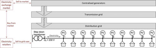
In the past, electricity flow was mono-directional from centralized generators to the transmission grid, from the transmission to the distribution grid, and from the distribution grid to grid users. Nowadays, due to the high deployment of DER, the power flow between the distribution grid and grid users, as well as between the transmission and the distribution grid can be bidirectional. When the electricity generation from RES exceeds the load at a certain distribution grid node, the surplus power is redistributed to other loads through the distribution lines.

The electricity retailers buy electricity in the electricity exchange (wholesale) market from centralized generators, and sell it to the grid users. Electricity retailers also buy energy surplus from grid users.

A grid user, who is directly connected to the electricity distribution grid, has the potential to contribute to the power quality and security of supply. Operation patterns of electrical loads of grid users could be adapted to contribute in peak load shaving (congestion management) by shifting the load from peak times to off-peak times (Purvins and Sumner 2013). Off-peak load also refers to DER generation surplus. DER consumption locally is of high interest to grid users as it keeps electricity costs low. Peak load shaving contributions to reducing the electricity distribution losses is another benefit to consider (Rahimi et al. 2013). In addition, load shifting could be managed in a way to optimize the purchases of electricity from the electricity exchange market in a cost-effective manner. The contribution to the power balance in the present article is addressed as far as it applies to the two-tariff electricity pricing. These potential contributions of load shifting could result in a reduction of electricity costs for grid users and therefore are addressed in the proposed methodology for energy management.

Energy management

The proposed energy management of electrical loads applies to distributed energy systems with a high deployment of DER. The management goals from the previous section can be summarized as follows:

1. Maximum utilization of DER in the local grid (local consumption of generation surplus)

2. Local grid support: peak load shaving/congestion management

3. Local grid support: reduction of electricity distribution losses

4. Cost-effective load shifting following the electricity price

The management is performed centrally at the neighborhood level. Neighborhood, for example, could comprise all grid users connected to the low-voltage side of a medium- to low-voltage substation. The instrument for the energy management is the controllable electrical load.

Centralized energy management could be provided by an electricity retailer or a demand-side aggregator who could (i) participate in the electricity exchange market with power demand bids (Campaigne and Oren 2016), and (ii) offer load shifting-based grid support services to the local Distribution System Operator (DSO) (Esmat and Usaola 2016).

Based on the energy situation in the neighborhood, the central management system will inform the grid users on the optimal shifting of electrical loads. The final load shifting is performed by the grid users following the suggestions from the central management system. Thus, the management decision is performed centrally and applied by decentralized energy management systems of individual grid users. Decentralized management systems have direct access to the controllable loads of grid users. This ensures a high utilization of flexible load resources in the neighborhood. Such management provides efficient performance of load shifting taking into account not only the interests of individual grid users but also the techno-economic interests of the whole neighborhood as well as the electricity distribution grid. Thus, the proposed management serves all involved grid users, and it is up to the grid users themselves whether to apply the suggested management efficiently. As concluded by Lu et al. (2011), such a combination of centralized and decentralized energy management systems may increase the performance of the Smart Grid.

The proposed energy management is developed for the automated management of controllable electrical loads. Such management can be applied not only to electrical loads but also to controllable electric generators. Good examples here are electric motors or generators in electrothermal systems – combined heat and power (CHP) plants and heat pumps (e.g., in solar thermal systems, air conditioners, geothermal heat pumps). The methodology can also be applied to storage systems with electricity as input and/or output energy type (e.g., electrochemical secondary batteries). The above-mentioned electrothermal systems are good candidates for automated electricity management since they include thermal energy storage. Thermal storage provides the energy system with flexibility in operation: the operation of electric motors may be shifted in time (e.g., 20 min later or earlier) without affecting the normal operation of the system. Normal operation is the operation of the thermoelectric system, which ensures that heating or cooling characteristics (e.g., temperature in a room, hot water temperature) are in an acceptable range.

Methodology

The proposed energy management can be structured as depicted in Figure 2. It comprises two calculation algorithms:

1. PV generation forecast calculation

2. Optimal load shifting planning calculation

Figure 2. The structure of the proposed energy management: Input/output data and calculation algorithms.

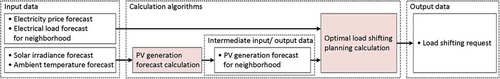
The first algorithm calculates the generation forecast of PV plants in the neighborhood. The calculated forecast provides the required input for the second algorithm: optimal load shifting planning calculation. The second one is the main algorithm. It plans optimal load shifting for the involved grid users taking into account the energy situation in the neighborhood one day ahead. Such management structure is applicable for electricity systems with PV plants.

The optimal load shifting planning calculation algorithm is described in detail in the following sections. The PV generation forecast calculation from solar irradiance and ambient temperature is presented and validated in Appendix A.

Optimal load shifting planning calculation

In this section, the methodology of the optimal load shifting planning calculation is described in detail. It calculates the load shifting request for grid users (Figure 2).

The optimal load shifting planning calculation starts when at least one of the following input data sets is updated: (i) the electricity price forecast, (ii) the neighborhood electrical load forecast, or (iii) the PV generation forecast for neighborhood (see Figure 3). Forecasted data is a data array of values one day in advance for every 10 min. The proposed methodology is developed for intraday energy management. Whenever the input data is updated, a new load shifting request is calculated. Ideally, all input forecast profiles are updated every 10 min. Intraday energy management allows adjusting load shifting every 10 min following changes in input data. Such management requires rapid action in load shifting planning. Therefore, it is applicable to controllable loads, the operation pattern of which can be automated.

Figure 3. Flowchart of the optimal load shifting planning calculation.

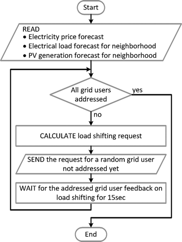
The aforementioned input data is required to assess the overall energy situation in the neighborhood and to address the management goals as efficiently as possible. The electricity price forecast is assumed to be the same for all grid users in a first approximation. The neighborhood electrical load forecast comprises all neighborhood grid users that are not involved in the load shifting. For example, the neighborhood could be formed of all grid users connected to the low-voltage side of a medium- to low-voltage substation. If the neighborhood has 50 grid users and only 10 of them are participating in load shifting, then the neighborhood load forecast is required from the remaining 40 grid users that are not involved in the load shifting. Moreover, the PV generation forecast is calculated for the whole neighborhood.

The algorithm calculates the optimal load shifting for individual grid users in terms of the load shifting request profile, which is calculated based on the aforementioned management goals. The resulting profile can contain load shifting request values of “–2”, “–1”, “1”, and “2” for the next 24 hr with a time resolution of 10 min. The values are determined from the electricity price and the residual neighborhood load as shown in Table 1. The residual load is the electricity load minus the PV gener“–2” and “–1” indicate times from which the load is suggested to be shifted. “2” and “1” indicate times to which load is suggested to be shifted. Load shifting during times of “–2” and “2” is strongly recommended. The sign of the load shifting signal is inversely proportional to the electricity price. At two-tariff electricity pricing, the signal is negative during the times of a high electricity price and it is positive during the times of a low price. Exception is Case #3, where there is negative residual load (generation surplus) during the times of a high price. The case of a low price and negative residual load will fall under Case #5.

Table 1. Decision table for load shifting request.

Case #	Price	Residual load	Load shifting signal	Action
1	High	Positive peak	−2	Shift load from these times; strongly suggested
2	High	Positive & Not peak	−1	Shift load from these times
3	High	Negative	+2	Shift load to these times; strongly suggested
4	Low	Any & Not off-peak	+1	Shift load to these times
5	Low	Off-peak	+2	Shift load to these times; strongly suggested

Peak and off-peak times of the residual load are determined from the theoretically maximum peak shaving capability of the addressed grid user. The energy management system knows the approximate capacity of flexible load on the side of the grid users from historical data. This capacity is used to calculate the theoretical maximum peak shaving for the next day assuming that the flexible load is completely flexible. From this theoretical profile, the value of “–2” is assigned to the times where the peak load is shaved, and the value of “2” refers to the times when off-peak is filled. An example of optimal load shifting profile is presented in the next section.

Such load shifting request profiles are calculated for individual grid users. Grid users are addressed one after another as shown in Figure 3. First, the load shifting request is calculated for the grid user at Node #1 (Figure 1). Once the request is calculated, the grid user receives it and applies load shifting according to this request. In order to proceed, feedback from the grid user at Node #1 about its load shifting planning is required (day-ahead electrical load forecast at Node #1 with load values for every 10 min). Once the feedback is received or a time delay of 15 sec has passed, the cycle repeats for the next grid user until all involved grid users are addressed. Electrical load forecasts from previously addressed grid users are taken into account for load shifting planning for the next grid user. In this manner, the risk of creating load peaks or off-peaks is avoided. Such a methodology strives to fulfill the energy management goals without needing to know the precise load shifting capacity in the neighborhood. Not all grid users involved in load shifting will be able to provide electrical load forecast. Load forecast of such grid users shall be included in the total neighborhood load forecast.

Sensitivity analysis

A sensitivity analysis of the proposed energy management methodology is applied for a radial distribution feeder with 10 grid users and 10 PV plants as depicted in Figure 1. Grid users are represented as households. The analysis is performed for 5 days.

Historical PV generation data (see Figure A.2 in Appendix A) is used as input data for the sensitivity analysis. The data is gathered from a PV power plant containing 24 × 80 W panels (1.92 kW in total) of 5 independent days in June with a time step of 10 min. The first value is registered each day at 22:50.

Load data is taken from historical measurements from the EEPOS project field test site in Langenfeld in Germany. The average daily load profile of three households (with two inhabitants in each) in June, which operate under a single uniform electricity tariff, is used for the analysis. This profile is assumed to be the same for all 5 days. The total electricity consumption implied by this profile is 4.54 kWh per day. In the analysis, the same profile is applied to all 10 grid users. The electricity consumption of 10 grid users in 5 days is depicted in Figure 4.

Figure 4. Input data: PV plant generation, load, residual load, electricity price.

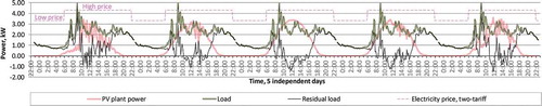
For simulation purposes, the PV plant size is doubled so that during high PV generation around noon, power surplus slightly exceeds 1 kW (see residual load in Figure 4). The shape of the PV generation profile remains the same. It can be noticed that it partly reduces the morning and evening peak loads. The PV capacity among grid users is distributed equally.

For the analysis, a two-tariff pricing for electricity is used. As presented in Figure 4, during the daytime from 6:00 to 22:00, the price is high and during night time from 22:00 to 6:00 it is low. Such two-tariff pricing is offered by some energy retailers in Germany. Two-tariff pricing is the first step in grid user participation in power balance.

Different load shifting capacities are used for the sensitivity analysis (see Table 2). The load flexibility in Table 2 is the capacity of controllable load expressed as a percentage of the average daily electricity consumption of each grid user. For example, in Scenario #2 each of the 10 grid users has the same capacity of flexible load: 2.5%. In absolute values, the feeder has 1.14 kWh as the total capacity of loads, the operation pattern of which can be controlled (a 0.114 kWh value for every individual grid user).

Table 2. Scenarios for flexible load capacities.

Scenario #	Load flexibility, %	Capacity, kWh
1	0.0	0.00
2	2.5	1.14
3	5.0	2.27
4	7.5	3.41
5	10.0	4.54

The optimal load shifting request profile is calculated and applied to grid users as described previously. Grid users are addressed one by one. The feedback from the already-addressed grid users is taken into account when addressing the next grid user.

An example of load shifting approaching the first grid user is depicted in Figure 5 for the first day and Scenario #4. The residual load of the neighborhood before and after load shifting is presented. The available flexible load capacity for this operation is 1/10 of 3.41 kWh (Table 2). The electricity price is as described before. The load shifting request value is set for every 10 min. For example, at 5:50 the request value is set to “1”. It stays “1” until 6:00. At 6:00 the load shifting request value is set to “−1”.

Figure 5. First day: Residual load, residual load after performed load shifting by the first grid user (Scenario #4), electricity price, load shifting request for the first grid user (Scenario #4).

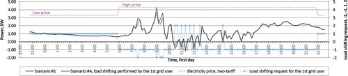
The load shifting request suggests optimal times for load shifting, but it does not provide any information about the actual amount of load that needs to be shifted. Hence, it is assumed in this analysis that grid users shift equal amount of their load in every hour where load shifting is applied. Such grid user behaviour may lead to overcompensation of generation surplus, e.g., at 11:40 in Figure 5. Similarly at time periods of “–2”, the peak load at 9:00 could be shaved more if the grid user knew that this is the highest peak of the day. However, having several grid users involved, the final load shifting in the neighborhood is expected to be relatively smooth.

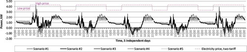
The resulted load shifting applying scenarios listed in Table 2 are illustrated in Figure 6. The generation surplus compensation and the peak shaving capability depend on the available capacity of the flexible load. Scenario #4 and Scenario #5 cover most of the power surplus (negative load) on all five days. At low power surplus, most of the flexible load capacity is used to fill low load hours during the night (e.g., from 22:50 to 6:00 on the first day). The load for filling off-peaks is taken mostly from the wide peak load hours in the evening (e.g., from 17:30 to 22:00 on the first day). The relatively narrow and high peak load during the morning hours is reduced as well.

Figure 6. Residual load (scenarios #1 to #5) and electricity price.

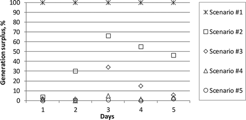
Figure 7 illustrates how different capacities of flexible load cope with the generation surplus. The reference value is the generation surplus in Scenario #1. The larger the capacity of flexible load, the more energy surplus it can compensate until the energy surplus reaches zero. On the second day applying Scenario #2, for example, the generation surplus is reduced by 70% (from 1.55 to 0.47 kWh). On the second day, the surplus is fully compensated applying flexible load capacities of Scenario #3. Higher generation surplus, as on day three, requires higher capacities of flexible load to complete the compensation.

Figure 7. Generation surplus compensation: Scenarios #1 to #5.

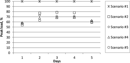
The peak load shaving results in relative values are presented in Figure 8. Daily peak load in Scenario #1 is a reference value and it is set to 100%. On the second day, for example, applying Scenario #2, the peak load is reduced to 77% if compared with Scenario #1 (from 2.90 to 2.24 kW). The first day and the fifth day are characterized by high peak reduction due to high and narrow morning peaks, compared with the other days. On the first and the fifth day, there is no noticeable difference in peak shaving among scenarios #2–#5 either; however, on other days, a higher capacity of flexible load leads to better peak shaving results.

Figure 8. Peak load shaving: Scenarios #1 to #5.

In order to assess the effect of the proposed energy management on electricity distribution losses, additional assumptions regarding technical parameters for the feeder depicted in Figure 1 are required. These parameters are taken from the study of Papaioannou, Purvins, and Demoulias (2014a) and are adapted to the needs of the grid user capacity:

1. The voltage of the single-phase transformer secondary winding – 230 V

2. An overhead Aluminium Conductor Steel Reinforced line (ACSR, stranding Aluminium/Steel – 6/1, diameter of individual wire – 1.68 mm)

3. The distances between neighboring nodes – 60 m

4. The power factor of grid user load, cosφ, – 0.7

The applied methodology for calculating the losses is described in the article of Papaioannou, Purvins, and Tzimas (2013).

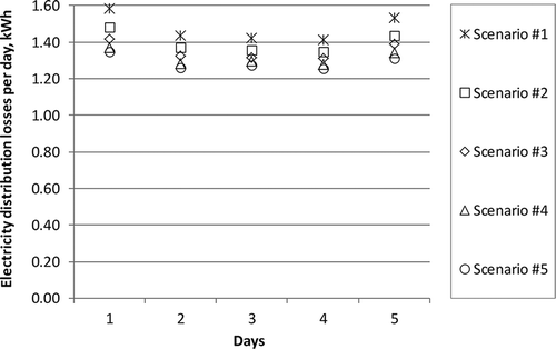
The reduction of electricity distribution losses in absolute values is shown in Figure 9. Losses are presented per day. On the first day, for example, the electricity losses in the feeder amount to 1.58 kWh in Scenario #1 (without flexible load). This amount of loss represents 5% of the total daily residual load in the feeder. On other days, these losses are also close to 5%. Load shifting as applied in scenarios #2–#5 results in a reduction of losses. During the first day, the electricity losses are reduced from 1.58 kWh to 1.35 kWh applying flexible load capacity of Scenario #5. In relative values, Scenario #5 may reduce losses as far as by 15% depending on the day. The chosen feeder parameters directly influence losses. The conductor line with a higher diameter will result in a reduction of losses due to lower resistance.

Figure 9. Electricity distribution losses per day: Scenarios #1 to #5.

This subsection concludes with an economic analysis from the grid user perspective under a two-tariff electricity pricing. The electricity price is an instrument to regulate grid user electricity consumption pattern. The load shifting’s financial benefit to the grid user is an important element that could motivate the grid user to contribute to load shifting.

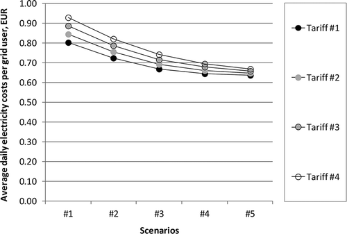
The electricity costs of the grid users are calculated at different electricity pricing tariffs as listed in Table 3. The electricity tariff #1 is chosen close to those values offered by energy service providers in Germany: 0.30 EUR/kWh from 6:00 to 22:00, and 0.25 EUR/kWh from 22:00 to 6:00. For every further scenario, the high price is increased by 0.03 EUR/kWh and the low price is reduced by 0.03 EUR/kWh. The feed-in tariff for PV generation is assumed as 0.13 EUR/kWh as currently practiced in Germany.

Table 3. Electricity pricing tariffs for grid users.

Electricity pricing tariff #	High price, EUR/kWh	Low price, EUR/kWh	Feed-in tariff, EUR/kWh
1	0.30	0.25	0.13
2	0.33	0.22	0.13
3	0.36	0.19	0.13
4	0.39	0.16	0.13

The average daily electricity costs per grid user applying different electricity pricing tariffs (Table 3) are presented in Figure 10. The load shifting results in a decrease of the electricity costs. Already a small amount of flexible load capacity (Scenario #2) reduces the electricity costs by 10–12% depending on the tariff. For example, the average daily electricity costs per grid user are reduced from 0.80 to 0.72 EUR by applying Scenario #2 and Tariff #1. Further increase in flexible load capacity is less effective. Scenario #5 (compared with Scenario #2) results in additional 10–16 percentage points to costs reduction depending on the electricity tariff.

Figure 10. Average daily electricity costs per grid user at different electricity pricing tariffs: Scenarios #1 to #5.

Discussion on analysis results

The sensitivity analysis shows that the proposed methodology of the energy management addresses the management goals efficiently through load shifting. The analysis is limited to an electricity system consisting of a radial distribution feeder with 10 grid users and 10 PV plants. The analysis results provide insight on the effect of different flexible load capacities on (i) generation surplus compensation, (ii) peak load shaving, (iii) the reduction of electricity distribution losses, and (iv) the reduction of electricity costs for grid users. The presented results are case-sensitive and should be used as indicative information. Each specific electricity system, e.g., on neighborhood/city level, should be studied separately in order to obtain precise results on load shifting benefits.

The high penetration of renewable and variable generation (like the electricity from PV plants and wind farms) raises needs for additional services and technologies to cope with generation surplus. Curtailment of generation, electricity grid reinforcements, expansion of cross-border electricity transmission, higher dispatch rates of flexible generators, and increased energy storage capacities are well-discussed means (Armaroli and Balzani 2011; Brancucci Martínez-Anido et al. 2013; Papaioannou et al. 2014b; Purvins et al. 2012; Shropshire et al. 2012). Decentralized load management systems could ease this effort coping with distributed generators locally. Compensating generation surplus locally is the first goal in the proposed energy management approach and it also contributes to all other goals, as it reduces loading of the electricity distribution lines as well as the losses. It also leads to cost-efficient energy management.

A rise in electricity consumption in the future may lead to a rise in peak load. This may require the reinforcement of the electricity grids (Purvins et al. 2011b). From the perspective of the DSOs, load shifting could be an attractive technique for highly loaded distribution grids due to peak shaving services, helping cope with overloads and congestions (Purvins et al. 2013).

The reduction of active losses in electricity distribution is an additional benefit to load shifting. It is also clear that the local consumption of generated electricity will lead to the reduction of electricity distribution losses due to the fact that less electricity will flow through distribution lines. Peak load shaving will also lead to the additional reduction of losses. This can be explained with an equation for calculating active losses in electricity lines:

(1)

Here, R is the active resistance of the electricity line and I is the current in the line. The active resistance (R) is constant, but the current (I) varies depending on the load of the line. The more electricity is transferred through the line, the higher the current. Equation (1) shows the exponential relationship between the current and the losses. For example, if the current doubles from one to two amperes, the losses will be four times higher. Highly loaded grids have higher electricity distribution losses due to higher currents. Due to this, it is in the interest of DSOs to reduce the peaks load. Cost benefits for DSOs are not analyzed, but are of high importance for the assessment of the feasibility of load shifting systems.

In total, electricity transmission and distribution losses may be around 13% depending on electricity grid properties and energy management (The World Bank 2014). In the European Union, this level has nowadays already decreased to about 7%, also due to DER impact. Losses are higher in the distribution lines due to lower voltages. Losses reduction in distribution lines due to load shifting will lead to loss reduction in other parts of the electricity grid as well.

Regarding electricity costs, it shall be said that the currently existing two-tariff pricing of electricity may not be sufficient to lead to active involvement of grid users in load shifting (Purvins and Sumner 2013). Therefore, it is important to involve other parties like DSOs, which may be interested to buy load shifting services. More dynamic electricity pricing may also increase the contribution of load shifting in power balance in the electricity system.

Additional load shifting services for DSOs not analyzed in this article are phase balance and voltage control. Phase balance refers to three-phase electricity systems. Balanced loads among phases (i) keep the electricity distribution losses down, (ii) improve voltage profile in the grid, and (iii) reduce the required distribution feeder capacity.

The voltage should be maintained in a specific range in order to ensure high power quality in the electricity system. Conventionally, voltage control is realized through switching autotransformer tap changers, rearranging power flows among transmission lines, or through reactive power injection in electricity system. The first two of these means are currently practiced mainly in transmission grids, which are meshed and automated. Distribution grids, however, are not automated and are usually radial. Therefore, the main means for voltage control in distribution grids is reactive power injection. In future distribution grids with higher deployment of DER, an additional need for voltage control systems may arise. At times of high generation and low load, the voltage in low-voltage grids may exceed the upper limit. Papaioannou and Purvins (2014) have studied this challenge and offer a methodology to calculate the maximum DER capacity in distribution feeders keeping the voltage in an acceptable range. In addition, Papaioannou, Purvins, and Tzimas (2013) have concluded that in low-voltage lines, the voltage can be managed efficiently not only by reactive power injection but also by load shifting.

Experts’ view on the discussed load shifting services is presented in Appendix B, which is a valuable asset to this discussion.

Effect on transmission grid

From the perspective of a Transmission System Operator (TSO), the approach to the management of flexible loads has evolved over the years. In the past, it was characterized by a top-down approach: TSOs decided to implement measures like peak load shaving on the power demand side with the ultimate goal to defer investments in the network capacity (ENTSO-E 2014). In this sense, the concept of load management is still addressed by TSOs. On the other hand, load management, introduced by the electricity sector liberalization, is characterized by a bottom-up approach: measures are implemented to incentivize grid users to become active in managing their consumption, obtaining in turn economic benefits. This also involves incentive payments designed to shift or reduce electricity consumption at times of high wholesale market prices or when system reliability is threatened. The goal is to reduce electricity consumption in times of high energy costs or network constraints by allowing grid users to respond to price or quantity signals or by increasing grid users’ awareness. Load management programs can change grid users’ consumption indirectly, i.e., grid users change their behaviour in response to price signals (or other types of incentives), or directly, i.e., consumption is shifted automatically through technical signals (GridTech project 2015).

In addition to creating value for grid users through rewarding schemes for changing their consumption behaviour, load management can help TSOs maintain security of supply and system adequacy. This can support TSOs in optimizing the utilization of infrastructure and investments in the grids (Norton et al. 2014). Further benefits provided by load management from a system’s perspective can be drawn in terms of integration and exploitation of renewable energy sources and consequent CO₂ emissions reduction, as well as in terms of ancillary services (e.g., power balance) provision and market competitiveness enhancement. This poses several regulatory issues that are out of the scope of the present article.

Conclusions

This article provides potential stakeholders with insight into the EEPOS approach on automated energy management. The presented management methodology applies to centralized energy management systems in neighborhoods and cities. It is developed for the management of controllable electrical loads/generators, the operation pattern of which can be automated. The following management goals have been addressed:

1. Maximum utilization of distributed electricity generation in local grid

2. Peak load shaving/congestion management in electricity distribution grid

3. Reduction of electricity distribution losses

4. Cost-efficient load shifting for grid users

The presented energy management methodology was described in detail. It comprises two main calculation algorithms:

1. PV generation forecast calculation

2. Optimal load shifting planning calculation

The methodology is tested with a hypothetical sensitivity analysis of an electricity distribution feeder with 10 grid users and 10 PV plants. Each grid user has an average daily electricity consumption of 4.54 kWh and each PV plant has a size of 0.38 kW (panel peak power). Such a system has a PV generation surplus slightly exceeding 1 kW on sunny or partly cloudy days. An analysis is performed for 5 independent days.

The analysis results show an efficient performance of the presented methodology addressing the aforementioned goals. On a partly cloudy day, the generation surplus can be compensated with a flexible load capacity of 5%. The capacity of flexible load is expressed as a percentage of the average daily electricity consumption of the grid users. On a sunny day, a higher capacity – a flexible load of 7.5% – is required to cover the PV generation surplus locally.

Peak load shaving results show efficient reduction of peak load even at low flexible load capacities. The peak is cut by 21–46% when applying a flexible load capacity of 2.5%. Further increase of flexible load capacity does not lead to significant results in peak shaving.

The reduction of electricity distribution losses depends on the technical parameters of the test feeder. The chosen parameters are: the voltage of single-phase transformer secondary winding – 230 V; an overhead ACSR line (stranding Aluminium/Steel – 6/1, diameter of individual wire – 1.68 mm); the distances between neighboring grid users – 60 m. The analysis results show a reduction of losses by 4–6% applying a flexible load capacity of 2.5%, and by 10–15% at the flexible load capacity of 10%.

The reduction of electricity costs for grid users is presented at different electricity pricing tariffs. At a high price of 0.3 EUR/kWh, a low price of 0.25 EUR/kWh, and a PV feed-in tariff of 0.13 EUR/kWh, the electricity costs are reduced by 10% on average by applying a flexible load capacity of 2.5%, and by 21% at the flexible load capacity of 10%.

The analysis results give a general idea on the effect of the presented energy management methodology. The results are case sensitive and should be used as indicative information. The methodology applied to other electricity systems will lead to different results. Thus, every individual system should be studied separately. However, there is a clear tendency for the proposed energy management to provide grid support services and cost-efficient energy management. Experts’ view of such energy management systems is presented in Appendix B.

The presented methodology will be implemented in the open source software OGEMA (Open Gateway Energy Management Alliance, http://www.ogema.org/) and will be tested in two field demonstrations: in Langenfeld (Germany) and in Helsinki (Finland).

Abbreviations

ACSR	=	Aluminum Conductor Steel Reinforced
DER	=	Distributed Energy Resources
DR	=	Demand Response
DSO	=	Distribution System Operator
EEPOS	=	Energy management and decision support systems for Energy POSitive neighborhoods
EoT	=	Equation of Time
GMT	=	Greenwich Mean Time
HRA	=	Hour Angle
LST	=	Local Solar Time
LSTM	=	Local Standard Time Meridian
LT	=	Local Time
MPTC	=	Maximum Power Temperature Coefficient
NOCT	=	Nominal Operating Cell Temperature
OGEMA	=	Open Gateway Energy Management Alliance
PV	=	Photovoltaic
TC	=	Time Correction factor
TSO	=	Transmission System Operator

Notes

^1. Installing new DR systems with minimum effort; technical support like quick reference guide.

^2. DR system equipped with common communication technologies and drivers ensuring interoperability with other energy management/monitoring systems.

^3. Easy setup of new (e.g., site-specific) DR systems; templates and examples provided for standard DR applications.

^4. Installation of additional applications or updating existing applications in DR system without interruption of the running DR processes.

^5. (Temporary) data saving; useful for statistical purposes or for restart of the system after unintended shutdowns.

^6. Security of consumer energy consumption data, meaning that data communication is encrypted and every effort is taken to prevent third parties from illegally following data communication.

^7. Rapid detection of operation failures of the DR system and notification via e-mail/ text messages.

^8. Multifunctionality may offer additional features like feedback on energy consumption, suggestions for energy saving, warning on possible malfunction conditions in end-user energy system, etc.

^9. User-friendly interfaces for easy (energy management) settings, for energy/power monitoring, etc.; interface accessible through personal computer, smartphone, or similar devices.

^10. In a centralized DR system, the DR decision (about optimal load shifting) of controllable grid-user loads/ generators is made centrally, e.g., on neighborhood/city level.

^11. In a decentralized DR system, the DR decision (about optimal load shifting) of controllable grid-user loads/ generators is made locally, e.g., in a household.

Appendix A. PV generation forecast calculation

This appendix presents and validates the methodology of PV generation forecast calculation. A PV plant is chosen to be the only DER generator in the neighborhood. The input data for the calculation is solar irradiance and ambient temperature forecast (Figure 2). The calculation result is the PV generation forecast for the neighborhood, which represents the required input for the optimal load shifting planning calculation (see Figure 2).

The influence of wind speed on the PV power calculation is taken into account as far as using the NOCT (Nominal Operating Cell Temperature) coefficient presented in PV panel datasheets (see IEC 61215 for more information). However, this coefficient limits the application of the proposed calculation to open-rack mounted PV panels. Shading of PV panels due to the shadows of nearby ground-standing obstacles like trees, buildings, or mountains is not considered.

Calculation of the PV forecast starts when at least one of the weather forecasts is updated, in terms of either (i) solar irradiance or (ii) the ambient temperature (Figure 2). These are day-ahead forecast profiles with values for every 10 min. To capture the PV generation peaks (in a partly cloudy day), the forecast of the solar irradiance requires peak values.

Since a neighborhood may contain many PV plants with different panel tilts and azimuth angles, the solar irradiance on the surface of each PV plant is calculated individually. In this case, only values for the solar irradiance on a perpendicular surface are required from the irradiance forecast.

A detailed description of the all calculation steps of the PV generation forecast profile follows below. The required input data for the calculation is solar irradiance on a perpendicular surface and the ambient temperature as mentioned previously, as well as the following technical characteristics of a PV plant:

1. Peak power of the PV panel

2. MPTC (Maximum Power Temperature Coefficient)

3. NOCT (Nominal Operating Cell Temperature)

4. PV panel tilt angle

5. PV panel azimuth angle

6. Longitude and latitude

7. Rated inverter power

8. Inverter efficiency

The actual power output of the PV plant (Pplant, W) can be obtained as described by Masters (2004).

(A1)

P_rated is the peak power of the PV panel in W; S_panel is the solar irradiance on the panel surface in W/m²; MPTC is Maximum Power Temperature Coefficient in % /°C (negative number); T_cell is the panel cell temperature in °C; and η_inv is the efficiency of the electrical power inverter in %.

The values for solar irradiance on the panel surface (S_panel) and panel cell temperature (T_cell) depend on the weather data and need to be calculated correspondingly. The solar irradiance on the panel surface (S_panel, W/m²) is a product of the calculation based on: (i) the solar irradiance on a perpendicular surface (S_incident, W/m²), (ii) the panel orientation (panel tilt angle, β_panel in degrees, and panel azimuth, Φ_panel in degrees), and (iii) the position of the Sun (Sun elevation, β_sun in degrees, and the Sun azimuth, Φ_sun in degrees):

(A2)

A panel lying flat on the ground has a tilt angle of zero, β_panel = 0°, and a vertical panel has a tilt angle of 90°. Regarding the azimuth angle, the vast majority of the installed PV panels are frontally aligned toward the equator. A panel in the southern hemisphere will be facing north with Φ_panel = 0°, and a module in the northern hemisphere will normally face directly south with Φ_panel = 180°.

In order to calculate the position of the Sun, the Local Solar Time (LST in hours) needs to be determined first:

(A3)

LT is the Local Time, in hours from 0 to 24, and TC is the Time Correction factor in minutes.

The TC factor takes into account the deviation of LST in a specific time zone. Such deviation occurs due to longitude variations. It also incorporates the Equation of Time (EoT) and is expressed as follows:

(A4)

Long is the PV panel longitude in degrees. LSTM is the Local Standard Time Meridian in degrees. It depends on the difference between the LT and GMT, Greenwich Mean Time (ΔT_GMT in hours), and is calculated as follows.

(A5)

EoT (in minutes) is an equation that adds the correction factor to specify the LST calculation. Such correction is required due to the eccentricity of Earth’s axial tilt while moving around the Sun.

(A6)

B is a variable in degrees that depends on the day of the year (d) and is calculated as follows:

(A.7)

Furthermore, LST is converted into degrees and represents the Hour Angle (HRA in degrees):

(A8)

HRA is 0° at solar noon. In the morning, HRA is negative, in the afternoon it is positive.

Another derived parameter is the declination of the Sun (δ), that is an angle in degrees formed between the plane of the equator and a line drawn from the center of the Sun to the center of the Earth. It can be calculated as follows:

(A9)

Knowing HRA, Sun declination (δ), and latitude (Lat in degrees) of the PV panel location, the Sun elevation (β_sun in degrees) can be obtained as

(A10)

The Sun elevation angle (β_sun) is 0° at sunrise and 90° when the Sun is directly overhead. The Sun azimuth angle (Φ_sun in degrees) depends on whether the LST value is bigger or smaller than 12 h:

(A11)

(A12)

Φ_sun’ is calculated as follows:

(A13)

Similar to the azimuth angle of the PV panel, the azimuth angle of the Sun (Φ_sun) is defined in compass directions. With North it is 0° and with South it is 180°.

From the equations above, it can be concluded that the solar irradiance on the panel surface (S_panel) depends on the day of the year, local time, the time zone, and the PV panel location (Lat and Long). Summer time is not taken into account in this calculation.

The PV cell temperature is the last unknown parameter for the actual PV plant power calculation. The majority of the PV cell temperature calculation equations gathered by Skoplaki and Palyvos (2009) contain coefficients that usually cannot be found in PV panel datasheets or are linked to specific PV panel technologies. Knowing this, an equation that contains only conventional coefficients usually specified in PV panel datasheets has been chosen for PV cell temperature (°C) calculation from the article of Skoplaki and Palyvos (2009):

(A14)

T_amb is the ambient temperature in °C and T_NOCT is the Nominal Operating Cell Temperature (NOCT) in °C.

Tian et al. (2012) have used Eq. (A14) in their PV model and have tested it for 20 PV panels. The results are consistent with the experimental data provided by manufacturers under a wide range of temperature and solar irradiance values. Equation (A14) is the last calculation step for obtaining the PV plant power.

To create the PV generation forecast profile, this calculation should be carried out for every value in the weather forecast profile. In neighborhoods with more than one PV plant, the PV generation forecast should be calculated for every individual plant. The sum of these calculated forecasts provides the PV generation forecast for the neighborhood. An update by a newly calculated PV generation forecast will initiate the optimal load shifting planning calculation as shown in Figure 2.

The methodology for PV plant power calculation is validated with historical data of a PV plant located in Kassel, Germany. The data is provided by an EEPOS project partner Fraunhofer IWES. The plant consists of 24 PV panels each of 80 W peak power (for a total of 1.92 kW) and one inverter with a rated power of 1.80 kW. The maximum efficiency of the inverter is 94.3%. MPTC and NOCT of the PV panels are −0.24%/°C and 51°C, respectively. The panels are fixed and open-rack mounted facing south with tilt angle 30°.

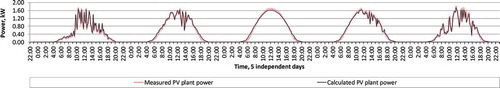
For validation purposes, the following historical data of five separate days in June (4^th, 9^th, 13^th, 18^th, and 22^nd) with 10-min intervals is used in terms of (i) the irradiance on the PV panel surface, (ii) the ambient temperature (Figure A.1), and (iii) the PV plant output power (Figure A.2). The data sets for each day begin at 22:50 on the previous day and end at 22:50 in the evening. Figure A.1 demonstrates how cloudiness in the first and in the fifth day reduces the amount of solar irradiance on the PV panel surface, as well as the ambient temperature. This directly affects the PV plant power output as depicted in Figure A.2. Historical PV plant power in Figure A.2 is presented together with the calculated PV plant power using the proposed methodology.

Figure A.1. Historical data of PV plant: Irradiance on PV panel surface and ambient temperature.

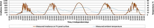
Figure A.2. Historical data of PV plant power output and calculated PV plant power.

The calculated value of the PV plant power is validated with that from the historical data: for this comparison, the following formula calculating the average relative error is used:

(A15)

P_measured.i is the PV plant power output value of historical measurement i; P_calculated.i is the calculated value of the PV plant power output under the same conditions as for the measurement i; and n is the quantity of measurements.

The average absolute error is 6.9% for values where the historical PV power exceeds 10% of the PV plant peak power. For values above 50% of the plant peak power, the average error decreases to 2.7%. For calculated individual values, which are close to zero (below 5% of the PV plant peak power), the absolute error exceeds 100% in most of the cases. The reason for this could be the high drop in inverter efficiency at low operating power. This drop is not taken into account in the proposed calculation.

The error for the calculated energy values is −2.5%, and it is obtained as follows:

(A16)

E_measured is the energy produced by the PV plant during five days (as presented in Figure A.2); and E_calculated is the calculated energy for the same days. The proposed PV plant power calculation is not as accurate as in more advanced PV simulations tools like the PV model developed by Papaioannou and Purvins (2012); however, it is considered sufficient for energy management systems in neighborhoods.

The validation was performed using historical weather data. An additional error to the calculated PV plant power will be added from the forecasted weather data.

Appendix B. Demand response survey results

This appendix comprises results on the ‘Demand response (load shifting) survey’ launched at the end of 2014 in the course of the EEPOS project. All questions in the survey refer to electrical demand response (DR) at the electricity distribution grid level. DR here refers to the management of controllable electrical loads (and generators) of consumers: load shifting, e.g., in households, commercial buildings, and the industry.

The aim of the survey was to collect a general experts’ opinion on the role of DR systems in an efficient transition of the current electricity systems toward Smart Grids. In total, 59 experts from 41 companies have completed the survey and shared their view. Most of the experts are researchers, engineers, consultants, or hold management positions in an energy domain.

The main points from the experts’ comments are added to the description of the survey results. In addition, the outcome of the technical session “Energy management in electricity systems” of the joint PINTA-OGEMA-EEPOS workshop (held on April 2014 in Kassel/Germany) is also included where relevant. Discussion topics in the technical session covered the same questions as the survey.

The content of this appendix should be treated thoughtfully when applied for the development of DR systems, keeping in mind that DR is not a widely applied service and thus can be interpreted by experts differently.

The survey results are based on six technical questions, which arose during the initial research in DR systems in the EEPOS project:

1. How would you rate the importance of demand response (DR) in efficient Smart Grid development?

2. How would you rate the priority of DR among other Smart Grid elements, like electric vehicles, energy storage, etc.?

3. How would you rate the importance of the following DR functions for local electricity grid support?

   • Congestion management/peak load shaving

   • Phase balance

   • Voltage control

4. How would you rate the importance of the following DR functions for local generators support?

   • Local consumption of generation surplus (generation–consumption matching)

5. How would you rate the importance of the following DR functions for electricity system support?

   • Frequency control (power balance)

6. How important are the following (advanced) technical features for each type of DR system?

   • Fast installation¹

   • Interoperability²

   • Easy setup³

   • Limited downtime⁴

   • Data logging⁵

   • Data encryption⁶

   • Fault/Error alarms⁷

   • Multifunctionality⁸

   • User-friendly interface⁹

Answer options on these questions were made available in a 5-point rating scale as listed in Table B.1.

Table B.1. Answer options for questions 1–6.

Questions	Answers
1, 3–5	1 = Not at all important, 2 = Slightly important, 3 = Moderately important, 4 = Very important, 5 = Extremely important
2	1 = No priority, 2 = Low priority, 3 = Medium priority, 4 = High priority, 5 = Essential
6	From Least to Most important [1 = Least important; 5 = Most important], and 0 as Not applicable

Questions 6 was organized for three different DR systems:

1. Centralized¹⁰ automated DR system without consumer engagement

2. Decentralized¹¹ automated DR system without consumer engagement

3. Decentralized semi-automated DR system with active consumer engagement

The results of the survey are presented in Figures B.1–B.3, showing the range of answers, the average answer value, and the standard deviation of answers. The latter measures the dispersion of values from the average and is calculated as

(B.1)

where x_i is the answer of expert i, x_avg is the average value of answers, and N is the quantity of answers.

Figure B.1 depicts the experts’ view on the importance and priority of DR systems. Experts rated DR as Very important (in average) for efficient Smart Grid development. The priority of DR systems among other Smart Grid elements (like distributed storage and electric vehicles) was considered as high on average. The answers are quite consistent for both questions: standard deviation of answers is close to one. Only few experts rated DR as slightly or not at all important with low or no priority.

Figure B.1. Results on questions 1 and 2: Experts’ view on the importance and on the priority of DR system [1 = Not at all important; 5 = Extremely important] [1 = Not priority; 5 = Essential].

Experts have attributed high potential to DR systems with regard to energy balancing if properly implemented and well regulated, especially in commercial buildings and in the industry. Moreover, they pointed out the necessity for (standardized) communications between DR system and grid as well as between DR system and market.

Figure B.2 depicts the experts’ view on potential DR services (i) for local electricity grid, (ii) for local generators, and (iii) for electricity system. The average rating for peak load shaving and generation–consumption matching is close to Very important, whereas for phase balance, voltage control, and frequency control it is close to Moderately important. Answers are quite different for rated functions and vary widely from Not at all important to Extremely important.

Figure B.2. Results on questions 3-5: Experts’ view on the importance of the following DR functions (i) for local electricity grid, (ii) for local generators and (iii) for electricity system support [1 = Not at all important; 5 = Extremely important].

Experts have attributed high potential to peak load shaving pertaining to the reduction of the overall expenses for electricity retailers. During peak load hours, electricity may sell at a high price on the electricity market. Thus peak load shaving will reduce the costs of electricity bought on the market and may reflect positively in the electricity bill for the consumer. For DSOs, peak load shaving can keep down the operating costs of local grids (by reducing electricity distribution losses) and prevent grid reinforcement.

Generation–consumption matching can also keep electricity costs low for the consumer. In addition, it can increase the capacity of local renewable generators, which the grid can handle efficiently without any need for a reverse power flow in the distribution grid (i.e., no power flow from the consumer to the grid). In general, local generation–consumption balance will require less power balancing resources in the rest of the electricity system.

Other potential DR functions – such as phase balance, voltage control, and frequency control – should at first be managed by electric utilities. Experts reported DR assets in frequency control as not too important as long as electricity system frequency is maintained by large centralized generators having enough inertia reserves. Big industrial loads are considered better candidates for frequency control if compared with household appliances.

Figure B.3 shows the experts’ view on the importance of the advanced technical features for three different DR systems. Regarding centralized automated DR systems without consumer engagement, the leading features with the highest average rate (close to 4) are Interoperability, Limited downtime, Data logging, Data encryption, and Fault/Error alarms. These features have a relatively high consistency in the experts’ opinion (with standard deviation close to one), except for Interoperability and Data encryption. Other features have an average rate ranging from 2.5 to 3 and are thus considered less important.

Figure B.3. Results on question 6: Experts’ view on the importance of the advanced technical features for different DR systems [1 = Least important; 5 = Most important; 0 as Not applicable].

A decentralized automated DR system without consumer engagement was rated similarly for Data logging, Data encryption, Fault/Error alarms, and Multifunctionality features. Fast installation, Interoperability, and User friendly interface were rated higher, whereas Limited downtime function was rated lower.

On the contrary, a decentralized semi-automated DR system with active consumer engagement shows slightly different results from the two other systems. Here, all the features except Limited downtime were voted on average close to 4 and above. Interoperability and User friendly interface have the highest average score with high uniformity in the experts’ rating.

Some experts reported a high need for an active engagement of the consumer in DR systems. Without such engagement, DR may not bring sufficient results. In addition, decentralized DR systems with consumer engagement should be applied in a way that does not lead to discomfort of the consumer. However, currently there are no attractive mechanisms to actively involve consumers in DR. Double electricity tariff may help accelerate DR system implementation.

As concluded by experts, the necessity and usefulness of DR strongly depend on the electricity system and load properties. For example, some experts recognized the importance of generation–consumption matching and frequency control functions of DR in isolated electricity systems only. However, the presented survey results can be used as indicative material for initial steps in DR research and development.

References

- Anees, A., and Y.-P.-P. Chen. 2016. True real time pricing and combined power scheduling of electric appliances in residential energy management system. Applied Energy 165:592–600. doi:10.1016/j.apenergy.2015.12.103.
- Armaroli, N., and V. Balzani. 2011. Towards an electricity-powered world. Energy & Environmental Science 4:3193–222. doi:10.1039/c1ee01249e.
- Basak, P., S. Chowdhury, S. Halder Nee Dey, and S. P. Chowdhury. 2012. A literature review on integration of distributed energy resources in the perspective of control, protection and stability of microgrid. Renewable & Sustainable Energy Reviews 16:5545–56. doi:10.1016/j.rser.2012.05.043.
- Brancucci Martínez-Anido, C., M. Vandenbergh, L. De Vries, C. Alecu, A. Purvins, G. Fulli, and T. Huld. 2013. Medium-term demand for European cross-border electricity transmission capacity. Energy Policy 61:207–22. doi:10.1016/j.enpol.2013.05.073.
- Campaigne, C., and S. S. Oren. 2016. Firming renewable power with demand response: An end-to-end aggregator business model. Journal of Regulatory Economics 50:1–37. doi:10.1007/s11149-016-9301-y.
- Chen, Y. H., S. Y. Lu, Y. R. Chang, T. T. Lee, and M. C. Hu. 2013. Economic analysis and optimal energy management models for microgrid systems: A case study in Taiwan. Applied Energy 103:145–54. doi:10.1016/j.apenergy.2012.09.023.
- ENTSO-E 2014. Scenario Outlook and Adequacy Forecast. https://www.entsoe.eu/publications/system-development-reports/adequacy-forecasts/Pages/default.aspx (accessed June, 2017).
- Esmat, A., and J. Usaola. (2016). DSO congestion management using demand side flexibility. Proceedings of CIRED Workshop, Helsinki, Finland, June 14–15.
- GridTech project 2015. Report on promising new innovative technologies to foster RES-Electricity and storage integration into the European transmission system within the time frame 2020-2030-2050. http://www.gridtech.eu/images/Deliverables/GridTech_D3.1_Report%20on%20promising%20new%20innovative%20technologies.pdf (accessed June, 2017).
- Khodabakhsh, R., and S. Sirouspour. 2016. Optimal control of energy storage in a microgrid by minimizing conditional value-at-risk. IEEE Transactions on Sustainable Energy 7:1264–73. doi:10.1109/TSTE.2016.2543024.
- Klebow, B., A. Purvins, K. Piira, V. Lappalainen, and F. Judex. (2013). EEPOS automation and energy management system for neighbourhoods with high penetration of distributed renewable energy sources: A concept. Proceedings of IEEE International Workshop on Intelligent Energy Systems (IWIES), Vienna, Austria, November 14.
- Li, H., A. T. Eseye, J. Zhang, and D. Zheng. 2017. Optimal energy management for industrial microgrids with high-penetration renewables. Protection and Control of Modern Power Systems 2:12. doi:10.1186/s41601-017-0040-6.
- Lu, S., M. A. Elizondo, N. Samaan, K. Kalsi, E. Mayhorn, R. Diao, C. Jin, and Y. Zhang. (2011). Control strategies for distributed energy resources to maximize the use of wind power in rural microgrids. Proceedings of Innovative Smart Grid Technologies (ISGT), IEEE PES, Hilton Anaheim, CA, July 24–29.
- Masters, G. M. 2004. Renewable and efficient electric power systems. Hoboken, NJ: John Wiley & Sons.
- Norton, M., H. Vanderbroucke, E. Larsen, C. Dyke, S. Banares, C. Latour, and T. V. Van. 2014. Demand side response policy paper. ENTSO-E, Brussels, Belgium.
- Pan, H., Y. S. Hu, and L. Chen. 2013. Room-temperature stationary sodium-ion batteries for large-scale electric energy storage. Energy & Environmental Science 6:2338–60. doi:10.1039/c3ee40847g.
- Papaioannou, I. T., and A. Purvins. 2012. Mathematical and graphical approach for maximum power point modeling. Applied Energy 91:59–66. doi:10.1016/j.apenergy.2011.09.005.
- Papaioannou, I. T., and A. Purvins. 2014. A methodology to calculate maximum generation capacity in low voltage distribution feeders. International Journal of Electrical Power & Energy Systems 57:141–47. doi:10.1016/j.ijepes.2013.11.047.
- Papaioannou, I. T., A. Purvins, and C. S. Demoulias. 2014a. Reactive power consumption in photovoltaic inverters: A novel configuration for voltage regulation in low-voltage radial feeders with no need for central control. Progress in Photovoltaics 23:611–19. doi:10.1002/pip.2477.
- Papaioannou, I. T., A. Purvins, D. Shropshire, and J. Carlsson. 2014b. Role of a hybrid energy system comprising a small/medium-sized nuclear reactor and a biomass processing plant in a scenario with a high deployment of onshore wind farms. Journal of Energy Engineering 140:04013005. doi:10.1061/(ASCE)EY.1943-7897.0000142.
- Papaioannou, I. T., A. Purvins, and E. Tzimas. 2013. Demand shifting analysis at high penetration of distributed generation in low voltage grids. International Journal of Electrical Power & Energy Systems 44:540–46. doi:10.1016/j.ijepes.2012.07.054.
- Purvins, A., I. T. Papaioannou, and L. Debarberis. 2013. Application of battery-based storage systems in household-demand smoothening in electricity-distribution grids. Energy Conversion and Management 65:272–84. doi:10.1016/j.enconman.2012.07.018.
- Purvins, A., I. T. Papaioannou, I. Oleinikova, and E. Tzimas. 2012. Effects of variable renewable power on a country-scale electricity system: High penetration of hydro power plants and wind farms in electricity generation. Energy 43:225–36. doi:10.1016/j.energy.2012.04.038.
- Purvins, A., and M. Sumner. 2013. Optimal management of stationary lithium-ion battery system in electricity distribution grids. Journal of Power Sources 242:742–55. doi:10.1016/j.jpowsour.2013.05.097.
- Purvins, A., H. Wilkening, G. Fulli, E. Tzimas, G. Celli, S. Mocci, F. Pilo, and S. Tedde. 2011b. A European supergrid for renewable energy: Local impacts and far-reaching challenges. Journal of Cleaner Production 19:1909–16. doi:10.1016/j.jclepro.2011.07.003.
- Purvins, A., A. Zubaryeva, M. Llorente, E. Tzimas, and A. Mercier. 2011a. Challenges and options for a large wind power uptake by the European electricity system. Applied Energy 88:1461–69. doi:10.1016/j.apenergy.2010.12.017.
- Rahimi, A., M. Zarghami, M. Vaziri, and S. Vadhva. (2013). A simple and effective approach for peak load shaving using battery storage systems. Proceedings of North American Power Symposium (NAPS), Manhattan, KS, September 22–24.
- Shropshire, D., A. Purvins, I. T. Papaioannou, and I. Maschio. 2012. Benefits and cost implications from integrating small flexible nuclear reactors with off-shore wind farms in a virtual power plant. Energy Policy 46:558–73. doi:10.1016/j.enpol.2012.04.037.
- Skoplaki, E., and J. A. Palyvos. 2009. Operating temperature of photovoltaic modules: A survey of pertinent correlations. Renewable Energy 34:23–29. doi:10.1016/j.renene.2008.04.009.
- Tang, W., Y. Zhu, Y. Hou, L. Liu, Y. Wu, K. P. Loh, H. Zhang, and K. Zhu. 2013. Aqueous rechargeable lithium batteries as an energy storage system of superfast charging. Energy & Environmental Science 6:2093–104. doi:10.1039/c3ee24249h.
- Tian, H., F. Mancilla-David, K. Ellis, E. Muljadi, and P. Jenkins. 2012. A cell-to-module-to-array detailed model for photovoltaic panels. Solar Energy 86:2695–96. doi:10.1016/j.solener.2012.06.004.
- Tyagi, V. V., A. K. Pandey, D. Buddhi, and R. Kothari. 2016. Thermal performance assessment of encapsulated PCM based thermal management system to reduce peak energy demand in buildings. Energy and Buildings 117:44–52. doi:10.1016/j.enbuild.2016.01.042.
- Wang, G., V. Kekatos, A. J. Conejo, and G. B. Giannakis. 2016a. Ergodic energy management leveraging resource variability in distribution grids. IEEE Transactions on Power Systems 31:4765–75. doi:10.1109/TPWRS.2016.2524679.
- Wang, Z., B. Chen, J. Wang, and J. Kim. 2016b. Decentralized energy management system for networked microgrids in grid-connected and islanded modes. IEEE Transactions on Smart Grid 7:1097–105. doi:10.1109/TSG.2015.2427371.
- The World Bank. Electric power transmission and distribution losses. Accessed June 2017. http://data.worldbank.org/indicator/EG.ELC.LOSS.ZS.
- Zhang, Y., A. Lundblad, P. E. Campana, F. Benavente, and J. Yan. 2017. Battery sizing and rule-based operation of grid-connected photovoltaic-battery system: A case study in Sweden. Energy Conversion and Management 133:249–63. doi:10.1016/j.enconman.2016.11.060.