Historical Context and Recent Advances in Exposure-Response Estimation for Deriving Occupational Exposure Limits

Abstract

Virtually no occupational exposure standards specify the level of risk for the prescribed exposure, and most occupational exposure limits are not based on quantitative risk assessment (QRA) at all. Wider use of QRA could improve understanding of occupational risks while increasing focus on identifying exposure concentrations conferring acceptably low levels of risk to workers. Exposure-response modeling between a defined hazard and the biological response of interest is necessary to provide a quantitative foundation for risk-based occupational exposure limits; and there has been considerable work devoted to establishing reliable methods quantifying the exposure-response relationship including methods of extrapolation below the observed responses. We review several exposure-response modeling methods available for QRA, and demonstrate their utility with simulated data sets.

Keywords:

• benchmark dose
• critical effect
• dose-response
• exposure-response
• modeling
• occupational

INTRODUCTION

The industrial hygiene community is focused on limiting risk, which is the probability of adverse response in exposed occupational populations. Until now, very few occupational exposure limits have been based on quantitative risk assessments (QRA) that have the goal of achieving a targeted level of risk. In the few instances where QRAs have been available, the resulting exposure limits typically represent decisions influenced by other factors such as economic or measurement feasibility.^(1,2) To characterize and disclose risks so that the resulting occupational exposure limit (OEL) better reflects the hazards involved and achieves an explicit low level of residual risk, QRA is required.^(3–5) The key step in QRA is estimation of the exposure-response relationship. Today, there are a variety of statistical tools available for exposure-response modeling that should be used to characterize risks whenever data permit.

We use “exposure” generically to refer to either the environmental concentration of a hazard or to the dose of the same hazard in a target tissue. In animal toxicology studies, responses are often measured as dichotomous end points (e.g., tumor presence), but can also be continuous (e.g., liver weight) or ordinal (e.g., pathology severity scores). While the exposure-response relationship in such studies is generally well characterized, differences in species, routes, and duration of exposure, and the relative potency of similar exposures in humans, are sources of significant uncertainty.

Epidemiology studies can also be used to describe the adverse responses of humans to workplace hazards. One major advantage of epidemiology data is that no species extrapolation is needed. As with animal studies, responses can be measured on a variety of scales (continuous: lung function; ordinal: disease severity; dichotomous: cancer incidence, mortality) but the exposure concentrations may need to be historically reconstructed and estimated. Humans are rarely exposed to a single hazard, and even when they are, the appropriate measure of exposure may not be known. Confounders and effect modifiers may need to be incorporated in exposure-response models, the distribution of unknown host risk factors may influence or be influenced by the exposures, and developing health effects may influence current exposure status. Whether animal or human studies are used as the basis, ultimately, estimates of exposure-response relationships are required for deriving scientifically sound risk-based OELs.⁽⁶⁾

When using toxicological or epidemiological studies, choices made in modeling the exposure-response relationship affect OEL development. When a single statistical model is chosen to derive the final risk estimate, while other plausible models that produce different risk estimates go unused, model uncertainty in the risk estimation process is effectively ignored. Understanding the modeling process and the associated uncertainties is essential when developing an OEL and has been discussed extensively in National Research Council's (NRC) Science and Decisions: Advancing Risk Assessment, also known as the “Silver Book,”⁽⁵⁾ the NRC's Science and Judgement in Risk Assessment, also known as the “Blue Book,”⁽⁷⁾ and the NRC's Risk Assessment in the Federal Government: Managing the Process, also known as the “Red Book.”⁽³⁾. Here, we focus on modeling and model uncertainty and describes a range of statistical methods to characterize modeling uncertainty in QRA. Key points of emphasis covered in this manuscript include:

• various exposure-response assessment techniques used for point of departure (POD) selection, usually in animal studies, each with inherent strengths and limitations; and

• new methods for OEL setting, improving on the traditional techniques.

BACKGROUND

Establishment of Point of Departure

We define the POD as the exposure associated with observed risks within or just below the range of observed data. In practice, this risk level is selected to be 10%, well above a typical target risk level of concern. As discussed below, using model averaging or semiparametric methods, it is possible to reliably estimate the dose associated with low levels of risk that are considerably lower than 10% with no extrapolation from a POD.

Once the POD and target risk estimate are determined, the approach used for establishing the OEL will depend on organizational policies and other considerations.⁽⁸⁾ One such consideration that we discuss in detail is the linear extrapolation from the POD to an exposure associated with a target risk level. Typically, this is performed by specifying a linear exposure-response relationship from the POD toward the origin (i.e., the point where there is no exposure and excess risk) and assuming the response follows this line down to the risk level of interest. Alternatively, an allowable effect is constructed by adjusting the POD downward through the application of a product of uncertainty factors that attempt to account for differences in exposure duration, variability, sensitivity, interspecies adjustments, and a number of other modifying factors. Derivation and application of uncertainty factors are discussed in greater detail in Dankovic et al.⁽⁹⁾

NOAEL/ LOAEL-based PODs

The idea of the no observed adverse effect level was introduced by Lehman and Fitzhugh.⁽¹⁰⁾ The NOAEL is the highest experimental exposure where there is no statistically or biologically significant change in the outcome of interest. Changes that are not considered adverse are not used as the NOAEL even if they achieve statistical significance. In contrast to the NOAEL, the lowest observed adverse effect level (LOAEL) is the lowest dose or concentration that has been shown to biologically or statistically increase the outcome of interest relative to responses in unexposed individuals. In most animal studies, the statistical power is limited for detecting the small effect sizes that might be expected. It has been estimated that the highest exposure group qualifying as a NOAEL is estimated as being equivalent, on average, to model-based benchmark dose estimates (BMD, see below) for a 10% excess risk.⁽¹¹⁾

One limitation in the NOAEL/LOAEL⁽¹²⁾ approach is that it ignores the shape of the exposure-response curve which would inform extrapolation to lower levels; this is because the NOAEL/LOAEL is constrained to be one of the levels of exposure selected in the experiment. Another limitation is that the number of replications at each level affects the ability of the NOAEL/LOAEL to detect differences between dose groups. In general, NOAEL/LOAELs should only be used to set OELs if the data are not adequate for exposure-response analyses. When it is necessary to use the NOAEL/LOAEL approach, special attention should be paid to the limitations of the approach and the choice of uncertainty factors.

PODs from Exposure-Response Models and the Benchmark Dose Approach

Exposure-response models move beyond the hypothesis testing strategy embodied by the NOAEL/LOAEL approach to utilize all of the information in the exposure-response relationship to predict risks continuously over the range of exposures. Exposure-response models are described by an expected response = f(d, X₁,X₂,…,X_c) and a distribution defining the variability of the responses. The expected response is defined as a function of dose d and possibly other risk factors of interest represented by the variables X₁,X₂,…,X_c. In animal toxicology studies, this is often simplified to expected response = f(d), and this function is estimated given experimental data.

The function f(d, X₁,X₂,…,X_c) is often assumed to have a known parametric form reflecting assumptions on the shape of the dose response-curve. Care must be taken so that the model describes the data adequately, where the adequacy of fit is typically assessed using a goodness of fit statistic. Models that do not adequately fit the data should not be used.

When multiple models adequately describe the data, the model that is ultimately used for an occupational risk assessment should be chosen on some a priori model-choice criterion. The Akaike information criterion (AIC)⁽¹³⁾ is a frequently used criterion to pick the “best model,” although other metrics are available. Different criteria can lead to different choices, and, when setting an OEL from a model, the method of picking the “best model” should be transparent.

When estimating the exposure-response relationship there are minimum data requirements. For dichotomous data, one requires at least one dose group whose response is neither the background rate nor 100%. If such data do not exist, then the exposure-response relationship will not be estimable as the data essentially miss intermediate levels of the exposure-response curve. It is possible that no significant exposure-response relationship has been observed and the use of the BMD may result in doses that far exceed the maximum experimental dose. In either situation the use of the NOAEL may be the only viable option.

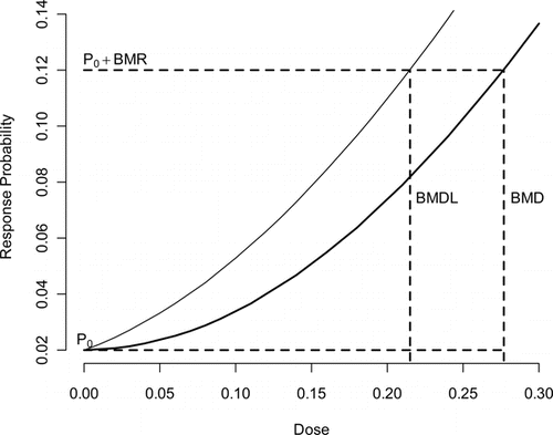
Given a suitable exposure-response model, one can use this model to estimate the BMD,⁽¹²⁾ which is described in Figure 1. The BMD is the dose associated with a specified change in the probability of response, known as the benchmark response (BMR). In estimating the POD, the BMR is often set to a predetermined level (typically 5% or 10%), which usually corresponds to the point where the BMD can be estimated without model extrapolation. The BMD is a point estimate, which does not reflect uncertainty in the true BMD; consequently, the 100(1-α)% benchmark dose lower bound (BMDL) is often used to define the POD. This quantity takes into account the sampling variability but does not reflect the uncertainty in the model selection process. When different models are used, the BMDL may differ, implying there is sensitivity of risk estimates to model form.

Figure 1 This figure shows the dichotomous specification of the added risk specification of the benchmark dose. The quantity P₀ is the probability of that response for unexposed subjects; P₀ + BMR represents the increased probability of response at the benchmark dose. Finally, the BMD is the dose associated with the point on f(d) associated with the population P₀ + BMR probability of adverse response.

The process for selecting the “best” exposure-response model involves uncertainty, especially when multiple models adequately fit the data and the BMDLs from these models vary by a large factor. This problem, which is called model uncertainty, has many different solutions of varying sophistication. Classically, a single model form was chosen a priori and was used to determine the POD.⁽¹⁴⁾ When using this approach one should follow the NRC Silver Book's⁽⁵⁾ minimum recommendation of reporting alternative plausible solutions to the risk manager as a context for understanding the uncertainty involved, where plausible implies a model is well supported by the data. The US EPA Benchmark dose guidance document⁽¹⁵⁾ recommends a decision logic approach in picking an estimate to use as a POD.

BMD for Continuous Responses

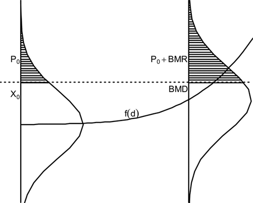
The BMD has also been defined for continuous responses such as weight or cholesterol.^(16,17) Instead of working with the probability of a dichotomous response, one creates probability statements based upon distributions of continuous endpoints and definitions of abnormal response, usually at an extreme of the continuum of responses. If large values of a response are considered adverse (e.g., cholesterol), the user must specify some value X₀ above which responses are considered abnormal in the population of interest. For the unexposed group, this response is assumed to occur with probability P₀ (baseline prevalence). The BMD is the dose where the probability of the abnormal response is P₀+BMR. This relationship is graphically described in Figure 2. Here the response is assumed to increase with dose. It is seen that the BMD is the dose that increases the probability of an abnormal response by the BMR. This is one method of computing the BMD, and other specifications are possible.

Figure 2 Graph of the continuous specification of the benchmark dose based upon the figure of Budtz-Jorgensen et al.⁽³⁸⁾ The quantity X₀ is the abnormal response cutoff, P₀ is the probability of that response for unexposed subjects, and P₀ + BMR is represents the increased probability of response at the benchmark dose. Finally, the BMD is the dose associated with the point on f(d) associated with the population P₀ + BMR probability of adverse response.

POD from Model Averaging of the BMD

Model averaging^(18–20) (MA) is a technique used to account for uncertainty in model selection. The main advantage to this method is that it explicitly accommodates the fact that multiple models may be consistent with a set of data by forming a BMD/BMDL as a weighted average of all of the models considered. This approach constructs a weighted average of the exposure-response curve from the competing models where weights are based upon on how well each model fits the data.

A thorough review of the reasoning behind different approximation methods can be found in Hoeting et al.⁽²⁰⁾ and Buckland et al,⁽¹⁹⁾ which describe the basis for a variety of model averaging approaches^(21–27) used in practice. In investigating approaches for estimating the BMD we focus on the frequentist model averaging estimates used by Wheeler and Bailer.⁽²⁷⁾

Early uses of model averaging in risk assessment focused on averaging individual model derived BMD/BMDLs,⁽²²⁾ which we term the “average-dose” approach. In the context of QRA, the set of BMD estimates is obtained from some finite set of possible models together with a set of positive weights that sum to one. The derived BMD and BMDL is then a weighted average of individual model estimates. The “average-dose” Bayesian MA estimate of the BMD and the BMDL can be constructed from the use of existing software packages, and are calculated by taking the weights formed from the AIC or the Bayesian information criterion BIC.

Wheeler et al.⁽²⁸⁾ showed that, while in many cases average-dose Bayesian model averaging was superior to picking the best model, its statistical properties were not optimal. Instead of focusing on averaging individual model-specific BMD estimates, other authors have investigated averaging the entire exposure-response curve^{(27, 29)} and estimating the BMD/BMDL from this average, which we name the “average-model” approach.

Wheeler and Bailer⁽²⁷⁾ used the frequentist MA methods of Buckland et al.⁽¹⁹⁾ to construct this average-model estimate, but a Bayesian approach⁽¹⁸⁾ can also be used. In simulation experiments,⁽²⁷⁾ the BMD/BMDL average-model estimates exhibited better statistical properties than the average-dose method. Based upon this study, we recommend that a large number of models be used for the model average, and, if cancer is the endpoint of interest, the quantal linear model should be included in the analysis to account for the possibility of a 1-hit cancer model. For our example (below), we look exclusively at model averaging for dichotomous outcomes. For continuous outcomes, we refer the reader to Shao and Gift.⁽²⁵⁾

POD from Semiparametric and Nonparametric Models and the BMD

Wheeler and Bailer⁽³⁰⁾ describe a Bayesian semiparametric method that uses a flexible spline construction for BMD analyses. In terms of its statistical properties, this method was shown to be superior to the model averaging method of Wheeler and Bailer.⁽²⁷⁾ The approach is fully Bayesian, which means one can easily include prior information on such things as the incidence of the response in historical controls. Even though semiparametric modeling avoids many of the model selection issues encountered in BMD modeling, significant, informed choices must still be addressed when using this method. Its use requires the choice of spline basis functions located at specific knot locations which should be selected before modeling begins.

Other fully semiparametric/nonparametric modeling methodologies have been recently developed for dichotomous and continuous data^(31–35) some of which overcome the knot selection problems of Wheeler and Bailer. These methods are fully nonparametric. Of these methods we note the continuous BMD method of Lin et al.⁽³⁵⁾ since they showed that, for large samples, their method would converge to the true underlying exposure-response curve, and, as a consequence, the BMD estimate would also converge to the true value. Wheeler et al.⁽³⁴⁾ provide a method for continuous outcomes that accounts for uncertainty in the specified response distribution as well as the exposure-response relationship.

As described above, in traditional BMD analyses, linear extrapolation from the POD to a target risk level is used to set the OEL. When using the MA “average-model” approach⁽²⁷⁾ or the semiparametric approach⁽³⁰⁾ this added linear extrapolation is unnecessary and the exposure concentration should be chosen directly at the level of risk specified (BMDR). When applied to actual data and investigated in simulation studies, these approaches have been found to well describe both the model and statistical uncertainties at excess risk levels considerably below the 5 or 10% level.⁽³⁶⁾

Epidemiological Data Issues

For human studies, many of the same techniques can be used with some modifications. Ideally, human studies have available detailed work histories that can be mapped to an historical exposure matrix such that each worker's estimated exposure history can be compiled and appropriate time-dependent exposure metrics calculated. Even when exposure history is available, significant measurement error is likely, degrading statistical power and potentially biasing estimates. In addition to the model uncertainty, exposure uncertainty would need to be considered in most epidemiology studies and in some cases it can be estimated.

Using human epidemiological data the exposure-response for the critical adverse effect can be modeled to low exposure levels. Here there is no need to define a POD, but uncertainty in the exposure response at low exposures can be a problem when the range of observed exposures is far above the range of interest. In this case, a linear low-dose extrapolation is a reasonable choice.^(4,5,37)

In human studies, model selection is more complex due to the presence of confounders or effect modifiers since there are often many ways the confounders can enter the model. One must also take into account many other considerations when constructing the exposure-response relationship. Table I gives a list of the most common of these.

Table 1 Common Impediments to Inference When Developing an Exposure-Response Relationship from Epidemiological Studies

Issue-Origins	Consequences	Fixes
Confounding bias -Other risk factors (RF) for outcome are associated with exposure^(^49^)	Under- or over-estimation of effects of exposure	Collect explicit information on confounding RFs or useful surrogates and model along with exposure effects.
Effect modification- Estimate of exposure effect depends on other RFs^(^49^)	RF-specific exposure response estimates result; response is not generalizable	Derive estimate for exposure response at some specified level of confounders, e.g., for population average smoking
Selection bias – Entry into study depends jointly on exposure status and outcome status^(^49^)	A problem for retrospective studies only; potentially fatal flaw when present	Achieve high participation rates; blind potential subjects and study operatives on study hypotheses; estimate maximum possible bias resulting
Healthy worker effect (HWE)- A special set of confounding RFs related to unknown health attributes of study participants that influence entry to study such as through hiring or fitness^(^49^)	The HWE can cause substantial underestimation of exposure effects depending on outcomes studied; can affect mortality and morbidity, cancer and non-cancer. The HWE may vary across demographic groups and over period of employment. If disease detection is superior in worker population overestimation of effect can occur.	Use internal comparison populations or, with external comparisons (e.g., national rates), estimate population differences.
Healthy worker survivor effect (HWSE)-Confounding that is time-dependent due to changing composition of workforce with duration of employment. For example, generally healthier workers may stay employed longer than others, long duration workers may smoke less, employed workers may have better healthcare.^(^50^)	Inappropriate comparisons may result depending on study design and analysis, usually causing underestimation of exposure effects.	Sometimes, if there is sufficient variation in exposure levels across study population, modeling employment duration together with exposure metrics can reduce this bias.
Reverse Causation- A special case of survivor bias in which the advent of the disease or health effect itself alters a worker's exposure status through employment termination or other health-induced job changes.^(^51^)	Cases with the outcome effect may exhibit less cumulative exposure than non-cases even though the outcome was caused by the exposure; a fundamental modeling assumption is violated and model fitting can be disabled.	This would be a fatal flaw in most study designs. It is much less important with long latency diseases where recent exposures are discounted (lagged). It occurs particularly with outcomes in which there is a preclinical phase of irritancy, impairment, or hyper-responsiveness to the exposure causing the outcome. Complex analytical approaches based on matching algorithms have been proposed and applied.
Variable susceptibility- A wide gradient of susceptibility resulting in a higher incidence of health effects cases initially from the most susceptible subjects, possibly depleting some high-susceptibility subpopulations over time producing lower overall susceptibility with advancing cumulative exposures^(^52^)	Exposure metrics show supra-linear associations with outcomes – apparent diminishing or attenuating effects with increasing exposure. Low exposure extrapolation pertains increasingly to higher susceptibility subpopulations. Similarly, a low susceptibility subpopulation could be present whose proportion of the population would increase over time.	Impose a linear exposure-response for a subset of observation time with less cumulative exposure, or attempt to accommodate a duration-dependent decline in susceptibility within the exposure-response model.

The effect of possible confounders or covariates on the response must be taken into account in a BMD calculation. Bailer et al.⁽²¹⁾ and Budtz-Jorgensen et al.⁽³⁸⁾ note that the BMD is often dependent upon these confounders. The BMD could be set in relation to specific confounders, and one may compute several associated BMDs for subpopulations of interest. Examples of BMD analyses in observational occupational studies includes respiratory disease in coal miners⁽²¹⁾ and Parkinsonism in welders.⁽³⁹⁾ In these studies, exposure-response models were developed, and the exposure-response function then applied to predicting distributions of the outcome variable.

As in animal studies, one can accommodate departures from linearity by fitting generally specified smooth curves based upon splines or fractional polynomials.^{(39, 40)} Spline applications in observational occupational studies include analyses of prostate and brain cancer mortality⁽⁴¹⁾ and aerodigestive cancer incidence⁽⁴²⁾ in workers exposed to metalworking fluids. Fractional polynomials accommodate non-linear exposure-response relationships, and may be a superior basis for risk assessment as they better account for uncertainty in the low exposure region.

As described above, Bayesian model averaging provides an alternative to splines as well as choosing a single model. Here, one is concerned not only with the shape of the exposure-response curve, but with how well the other covariates of interest are specified and modeled and the number of models increases exponentially as the number of covariates increase. Examples of model averaging in human environmental or occupational studies include lung cancer associated with arsenic in drinking water⁽²⁹⁾ and respiratory disease in coal miners.⁽²³⁾

METHODS

To compare the utility and results of various exposure-response modeling strategies for finding the critical dose when developing an OEL, an example is followed through various modeling options and critical exposures using several alternative techniques.

Datasets

Hypothetical animal inhalation toxicology data sets were constructed (Tables II and III). Here the responses are dichotomous, i.e., the data are represented as the number of animals exhibiting an adverse response out of a number of animals exposed at particular level. Inhalation doses are expressed in ppm and incidence of adverse responses tallied as number of animals with the adverse effect for each dose. Tables II and III illustrate data with different exposure-response properties.

Table 2 Dose Response Dataset I

Observation	Concentration (PPM)	# on test	# exhibiting the adverse response
1	0	20	1
2	12.5	20	1
3	25	20	4
4	50	20	8
5	100	5	5

Hypothetical dichotomous data set used as an example throughout the text to illustrate various methodologies in finding the critical dose.

Table 3 Dose Response Dataset II

Observation	Concentration (PPM)	# on test	# exhibiting the adverse response
1	0	10	0
2	10	10	0
3	20	10	3
4	40	10	4
5	80	10	6

Hypothetical dichotomous data set used as an example for Benchmark Dose estimation where there is significant model uncertainty when estimating the dose response.

Estimating the NOAEL/LOAEL

Data from observations 1, 2, and 5 in Table II were used for this illustration. The highest dose with no statistically significant response was determined to be the NOAEL. The lowest dose with a statistically significant response was determined to be the LOAEL. The Fischer's exact test, with a Bonferoni adjustment, at the α = 0.05 level was used to test for statistical significance.

Estimating the BMD

For the data in Tables II and III, we perform a BMD analysis for the probit, multistage, Weibull, gamma, log probit and quantal linear models available in the EPA Benchmark dose software system (BMDS 2.5)⁽⁴³⁾ using all dose levels for these data and the Dragon Excel spreadsheet BMDS wizard that is provided with the BMDS software. With all dose groups considered, the BMR is set to 10% and added risk is used in determining the BMD.

Estimating the Average-Dose Bayesian Model Average

The average-dose model BMD and BMDL estimates are constructed from the weights constructed using the AIC criterion. This is done using seven models available in the EPA BMDS model suite for dichotomous data described in Tables II and III. The weights are computed using the AIC calculation method of Wheeler and Bailer⁽²⁷⁾ and not the BMDS method.

Estimating the Average-Model Model Average

We use the model averaging for dose response (MADr) software package⁽⁴⁴⁾ to compute the MA according to the method of Wheeler and Bailer.⁽²⁷⁾ We use all of the models that were fit using the BMDS suite described above, and the AIC criterion for the weighting. The model choice is done for continuity with the above examples. In practice, we recommend the exclusion of the Multistage model and inclusion of the logistic and log-logistic models (rationale is fully described in Wheeler and Bailer⁽³⁶⁾). To use this approach, the MADr package or similar software is required.⁽⁴⁴⁾ The software is relatively easy to use, but users should have a good understanding of the implications of model selection when attempting model averaging.

Table 4 BMD Model Estimates

	BMD	BMDL	X^2 GOF P-Value	AIC	MA Weights^A	AIC^A
Probit	21.2	16.4	0.77	68.21	0.44	68.21
Multistage	21.9	12.1	0.76	68.49	0.14	70.49
Weibull	26.4	14.1	0.56	70.13	0.17	70.13
Gamma	25.4	13.5	0.48	70.72	0.13	70.72
Log Probit	25.4	14.3	0.40	71.31	0.09	71.31
Quantal Linear	10.9	7.2	0.19	73.54	0.03	73.54
MA Average Dose	22.8	14.5	NA	NA	NA	NA
MA Average Model	23.0	12.3	0.50	NA	NA	NA
Semiparametric	18.6	9.2	NA	NA	NA	NA

Computed benchmark doses across various estimation methodologies where the BMR = 10%, This is done using seven models available in the EPA BMDS model suite for dichotomous data described in Table II as well as the semiparametric method of Wheeler and Bailer.^{(30) A} The weights are computed using the AIC calculation method of Wheeler and Bailer⁽²⁷⁾ and not the BMDS software.

Estimating the BMD using Semiparametric Modeling

We estimate the BMD using the semiparametric method of Wheeler and Bailer.⁽³⁰⁾ Following that work, knots were placed at 0, 12.5, 45, and 100% of the maximum dose. The software code used for this analysis is freely available from the authors.

RESULTS/DISCUSSION

NOAEL/LOAEL

Given the full data set described in Table III, the NOAEL/LOAEL approach is not appropriate, as an exposure-response curve is estimable. However, if one were only given observations 1, 2, and 5, the NOAEL/LOAEL approach would be a reasonable choice because the reduced data set would not be adequate to support modeling.

Using only observations 1, 2, and 5 from Table II, the null hypothesis of no difference in mean cannot be rejected at dose 2.5 ppm. Consequently, the NOAEL for this data set is 12.5 ppm, with the LOAEL being 100. Both the NOAEL and LOAEL are dependent entirely on the dose spacing and numbers of events in the given data.

BMD

Using the dose-response data in Table II, BMDs were calculated (Table IV). One can see that depending on the model, the estimated BMD is between 10.9 ppm and 26.4 ppm with lower confidence limits on the BMD (i.e., BMDL) (here one-sided 95% confidence intervals) being between 7.2 ppm and 16.4 ppm. The BMDLs from this example do not vary more than a factor of 2.3.

Using the data from Table III, however, the BMDLs vary by almost a factor of 5 (Table V). Though one particular model fit is dramatically different from the others, Table V shows that all models describe the data adequately. Here, the BMDL computed from the Probit model is 16.2 ppm which is 4.9 times greater than the BMDL from the Log Probit, which is computed to be 3.3 ppm. As with the first data set, all of the models fit the data (as measured by a goodness of fit statistic). A natural question arises as to which BMD is appropriate as an estimate of the POD dose which will then be used to establish the OEL.

Table 5 BMD Model Estimates

	BMD	BMDL	X^2 GOF P-Value	AIC	MA Weights^A	AIC^A
Quantal Linear	8.7	5.8	0.78	43.97	0.341	45.97
Log Probit	13.0	3.3	0.66	45.30	0.176	47.38
Gamma	11.6	5.9	0.59	45.80	0.137	47.80
Weibull	11.0	5.9	0.59	45.85	0.133	47.85
Multistage	9.4	5.8	0.61	45.96	0.126	47.96
Probit	22.1	16.2	0.22	48.72	0.087	48.72
MA Average Dose	11.5	6.3	NA	NA	NA	NA
MA Average Model	11.1	5.3	0.40	NA	NA	NA
Semiparametric	15.1	8.5	NA	NA	NA	NA

Computed benchmark doses across various estimation methodologies where the BMR = 10%. This is done using seven models available in the EPA BMDS model suite for dichotomous data described in Table III as well as the semiparametric method of Wheeler and Bailer.^{(30) A} The weights are computed using the AIC calculation method of Wheeler and Bailer⁽²⁷⁾ and not the BMDS software.

For the data given in Table II, where the BMDLs of the plausible models differ by less than a factor of 3, the model with the lowest AIC normally would be chosen as the basis of the POD estimate.⁽¹⁸⁾ However, in the second data example this is not the case, and the decision logic would suggest the model with the lowest BMDL be used. As seen in these two examples, such an approach may lead to PODs that are not based upon any probabilistic quantification of the true model uncertainties involved and are based upon a very different rationale. A typical model selection and uncertainty process is summarized in Table VI. In this standard decision matrix for determining PODs, model uncertainty issues remain, and selecting one model has been found to underestimate the true BMD leading to potential dangers in model selection approaches.^(45,46)

Table 6 OEL Flowchart Showing Step-by-Step Process for Calculating the POD Using the BMD and a Suite of Models

	BMD Step	Action
1	Choice of models to be fit	Before the analysis develop a modeling approach that takes into account possible curvature that might be realistic. Models should be chosen on the basis of some a priori scientific rational (e.g., biologically relevant for carcinogenesis).
2	Fit models and estimate the BMD/BMDL using a prespecified BMR.	Given the model suite fit all models chosen and estimate the BMD/ BMDL at a prespecified BMR and confidence limit (typically taken to be BMR = 10% and confidence limit = 95%).
3	Select the best model given the data.	Using a statistical test (typically the Pearson chi-squared goodness of fit statistic) determine if the model adequately fits the data using some significance level (often.1) chosen prior to the analysis. Then from the remaining models use some predefined criterion (e.g., AIC) to pick the model to estimate the BMD/BMDL.
4	Calculate the POD from the BMD/BMDL.	With the best model chosen, use the BMD/BMDL to calculate the POD.

Table 7 OEL Estimation Methods

Method	Data Requirements	Considerations for use	Epidemiological Considerations	Caveats
NOAEL	Minimal data requirements	Use if no other method is appropriate or available.	Location and number of dose groups/exposure-strata is important.	Does not model the dose response curve and suffers from experimental design (dose-spacing) issues.
Traditional BMD	A minimum of two non-background responses with one partial response (i.e., not 100%)	Use if following current standard of exposure-response modeling.	Requires more sophistication on the modeler's part.	Overly optimistic inference poor coverage when true model is not known
Average Dose MA BMD	Same as traditional BMD	Use if output from standard exposure-response software allows this approach.	Potentiality for a large number of models to be averaged	Simple to implement with existing software but the method has poor coverage.
Average Model MA BMD	Same as traditional BMD	Use if computational resources allow for its implementation	Presently not extended for observational studies	Near nominal coverage for most situations. Requires non-standard (though readily available) software to implement.
Semiparametric BMD	Same as traditional BMD	Use if computational resources allow for its implementation.	Presently not extended for observational studies	Requires sophisticated software to implement.
Biologically Based Methods	Depends on the model more than empirical models.	Sufficient information exists on mode of action.	Sufficient info on biological features of model available in humans.	May allow better characterization of endpoint but requires knowledge of the mode of action. Still requires specification of which biological component is impacted by exposure.

List of the methods that can be used to develop an OEL; these methods are arranged in order of complexity as well as ability to account for model uncertainty. Here the NOAEL/LOAEL approach is the least complex and least able to account for uncertainty in the model form and the semiparametric methods are the most complex and most able to account for model uncertainty.

Average Dose Bayesian Model Averaging

For the first dataset the model fits are in Table IV, we construct the average-dose BMD and BMDL estimates from the weights constructed using the AIC criterion. From these weights, as well as the BMD and BMDL estimates found in that table, the dose model average BMD can be calculated as 22.8 ppm and the BMDL as 14.5 ppm. Table V gives the estimates for the second data set where the BMD is calculated to be 11.5 ppm with a BMDL of 6.3 ppm. While these estimates are similar to the single model estimates they take into account the model uncertainty by combining separate model fits.

Average-Model Model Averaging

As can be seen in Table IV for the first hypothetical dataset, the MA BMD is calculated to be 23.0 ppm with the lower bound estimated at 12.3 ppm, which is comparable to the individually estimated BMDs and BMDLs. Similarly, we look at the model-averaged estimate of the second hypothetical dataset, where the BMDLs differed by a factor of 5. Table V shows the BMD estimate to be 11.1 ppm with a BMDL of 5.3 ppm. Here this approach would result in a POD estimate greater than the approach using AIC to pick the “best” model.

Semiparametric Modeling

Using the semiparametric approach for the first hypothetical dataset, for a BMR of 10%, the BMD is estimated to be 18.6 ppm with a BMDL of 9.2 ppm (Table IV). For the second hypothetical dataset the BMD is estimated to be 15.1 ppm with a BMDL of 8.5 ppm (Table V), which is similar to the MA approach, but much greater than the BMD obtained from the default US EPA approach. A software implementation of the semiparametric modeling approach for dichotomous data is available from the authors.

Comparison of Modeling Results

Comparing target risk estimates across the modeling techniques applied here, the impact on the values used to potentially set OELs can be seen. For the data in Table II, estimating the exposure corresponding to a target risk level of 1/1000 using the semiparametric and average-model averaging approaches produce estimates that are very close to the POD plus linear extrapolation approach. The average model concentration corresponding to 1/1000 risk is estimated to be 0.58 ppm with lower confidence level (LCL) of 0.21 ppm. The semiparametric approach estimates the concentration at 1/1000 risk is 0.55 ppm with the LCL being 0.11 ppm. The linear extrapolation from the “best model” estimate of POD (BMDL) is 0.16 ppm (these values are found, assuming linearity, by dividing the 10% BMDL by 100 to get a risk estimate of 1/1000). The average model estimate is slightly higher than the linear extrapolated estimate and the semiparametric estimate slightly lower, but both are very much in line with the POD plus linear extrapolation estimate.

For the data in Table III, a different result is seen. The average model averaging estimate of the concentration corresponding to a 1/1000 risk is 0.15 ppm with a LCL of 0.08 ppm, while the semiparametric method estimates the concentration at 1/1000 risk to be 3.2 ppm with a LCL of 0.28 ppm. These are compared to the value of 0.033 ppm (log-probit), which is the concentration corresponding to 1/1000 risk using the recommended EPA approach. The EPA decision logic approach yields a concentration that is almost three times lower than the model average approach and 10 times lower than the semiparametric approach.

As shown with the examples above, even relatively simple data sets require a number of modeling decisions before a risk-based OEL can be derived. Table VII reviews the analysis and modeling options and gives a summary of data requirements, considerations and caveats.

When using model averaging or semiparametric/nonparametric methods, our recommended approach is a significant departure from past recommendations.⁽¹⁵⁾ Setting the BMR at 10% and using the BMDL as the POD with linear extrapolation to the risk level of interest has a long history, and it is supported by multiple studies showing that the BMD is often in the range of the NOAEL.^(11,47) We stress that this past recommendation is based on the observation that this risk level is approximately the point where models can reliably be fitted to the observed data, and, when one model is used, model extrapolations for lower risk levels can be overly precise.⁽²⁸⁾ Further, competing models may have orders of magnitude difference in the BMD/BMDL only increasing the uncertainty in the risk estimate. For an in-depth look at some methods addressing model uncertainty, we refer the reader to the book Uncertainty Modeling in Dose Response: Bench Testing Environmental Toxicity.⁽⁴⁸⁾ However, with advent of methods that account for uncertainty in the exposure-response curve, direct extrapolation from the exposure-response curve at the target risk level is well supported. As all competing models are included based upon some probability of their correctness given the experimental data, the estimate is based upon combining results over a set of model forms (model average) or possible curves (semiparametric/nonparametric), and it is much more reliable in the low risk/low dose region. We recommend that risk assessors directly estimate risks at low levels using these methods.

CONCLUSION

Risk assessors have a wide array of statistical tools to assess occupational risks. As shown with the examples above, risk assessors should use the most appropriate statistical methodology to estimate risks and quantify relevant uncertainties. Employing techniques that explicitly take into consideration the model uncertainty are preferred over selecting the “best model” approaches. However, decisions on which exposure-response analysis pathway to follow are often limited primarily by the quality and characteristics of the data set.

For risk management decisions, exposure-response modeling should become the cornerstone of quantitative OEL development. Advances in exposure-response modeling provide greater confidence in resulting OELs.

DISCLAIMER

The findings and conclusions in this report are those of the author(s) and do not necessarily represent the views of the National Institute for Occupational Safety and Health.

REFERENCES

- Castleman, B.I., and G.E. Ziem: Corporate influence on threshold limit values. Am. J. Ind. Med. 13(5):531–559 (1988).
- Ziem, G.E., and B.I. Castleman: Threshold limit values: historical perspectives and current practice. J. Occup. Med. 31(11):910–918 (1989).
- National Research Council: Risk Assessment in The Federal Government: Managing The Process. Washington, DC: National Academies Press, 1983.
- National Research Council: Understanding Risk: Informing Decisions in a Democratic Society. Washington, DC: National Academies Press, 1996.
- National Research Council:Science and Decisions: Advancing Risk Assessment. Washington, DC: National Academies Press, 2009.
- “Occupational Safety and Health Administration: Hazard Communication Standard; Final Rule”. Federal Register 7717574–17896.
- National Research Council: Science and Judgement in Risk Assessment. Washington, DC: National Academies Press, 1994.
- Waters, M., L. McKernn, A. Maier, M. Jayjock, V. Schaeffer, and L. Brosseau: Exposure estimation and interpretation of occupational risk: Enhanced information for the occupational risk manager. J. Occup. Environ. Hyg. Supplement 1: S99–S111 (2015).
- Dankovic, D.A., B.D. Naumann, A. Maier, M.L. Dourson, and L. Levy: The scientific basis of uncertainty factors used in setting occupational exposure limits. J. Occup. Envrion. Hyg. Supplement 1: S55–S68 (2015).
- Lehman, A.J., and O.G. Fitzhugh: 100-fold margin of safety. Assoc. Food Drug Off. US Q. Bull. 18:33–35 (1954).
- Wignall, J.A., A.J. Shapiro, F.A. Wright et al.: Standardizing benchmark dose calculations to improve science-based decisions in human health assessments. Environ. Health Perspect. 122(5):499–505 (2014).
- Crump, K.S.: A new method for determining allowable daily intakes. Fund. Appl. Toxicol. 4(5):854–871 (1984).
- Akaike, H.: A new look at the statistical model identification. IEEE Trans. Automatic Control 19:716–723 (1974).
- U.S. Environmental Protection Agency:“The Risk Assessment Guidelines of 1986.” Washington, DC: U.S. Environmental Protection Agency, 1986.
- U.S. Environmental Protection Agency:“Benchmark Dose Technical Guidance.” [Online] Available at http://www.epa.gov/raf/publications/pdfs/benchmark_dose_guidance.pdf, 2012).
- Kodell, R.L., and R.W. West: Upper confidence limits on excess risk for quantitative responses. Risk Anal. 13(2):177–182 (1993).
- Crump, K.S.: Calculation of benchmark dose from continuous data. Risk Anal. 15:79–89 (1995).
- Raftery, A.E.: Bayesian model selection in social research. Sociol. Methodol. 25:111–163 (1995).
- Buckland, S.T., K.P. Burnham, and N.H. Augustin: Model selection: an integral part of inference. Biometrics 53:603–618 (1997).
- Hoeting, J.A., D. Madigan, A.E. Raftery, and C.T. Volinsky: Bayesian model averaging: a tutorial (with comments by M. Clyde, David Draper and E. I. George, and a rejoinder by the authors). Statist. Sci. 14:382–417 (1999).
- Bailer, A.J., L.T. Stayner, R.J. Smith, E.D. Kuempel, and M.M. Prince: Estimating benchmark concentrations and other noncancer endpoints in epidemiology studies. Risk Anal. 17: 771–779 (1997).
- Kang, S.H., R.L. Kodell, and J.J. Chen: Incorporating model uncertainties along with data uncertainties in microbial risk assessment. Regul. Toxicol. Pharmacol. 32(1):68–72 (2000).
- Noble, R.B., A.J. Bailer, and R. Park: Model-averaged benchmark concentration estimates for continuous response data arising from epidemiological studies. Risk Anal. 29(4): 558–564 (2009).
- Piegorsch, W.W., L. An, A.A. Wickens, R. Webster West, E.A. Peña, and W. Wu: Information‐theoretic model‐averaged benchmark dose analysis in environmental risk assessment. Environmetrics 24(3):143–157 (2013).
- Shao, K., and J.S. Gift: Model uncertainty and Bayesian model averaged benchmark dose estimation for continuous data. Risk Anal. 34(1):101–120 (2014).
- Simmons, S.J., C. Chen, X. Li et al.: Bayesian model averaging for benchmark dose estimation. Environ. Ecol. Statist. 22(1):5–16 (2015).
- Wheeler, M.W., and A.J. Bailer: Properties of model-averaged BMDLs: a study of model averaging in dichotomous response risk estimation. Risk Anal. 27(3):659–670 (2007).
- Wheeler, M.W., and A.J. Bailer: Comparing model averaging with other model selection strategies for benchmark dose estimation. Environ. Ecol. Statist. 16(1):37–51 (2009).
- Morales, K.H., J.G. Ibrahim, C.J. Chen, and L.M. Ryan: Bayesian model averaging with applications to benchmark dose estimation for arsenic in drinking water. J. Am. Statist. Assoc. 101: 9–17 (2006).
- Wheeler, M., and A.J. Bailer: Monotonic Bayesian semiparametric benchmark dose analysis. Risk Anal. 32(7):1207–1218 (2012).
- Guha, N., A. Roy, L. Kopylev, J. Fox, M. Spassova, and P. White: Nonparametric Bayesian methods for benchmark dose estimation. Risk Anal. 33(9):1608–1619 (2013).
- Piegorsch, W.W., H. Xiong, R.N. Bhattacharya, and L. Lin: Nonparametric estimation of benchmark doses in environmental risk assessment. Environmetrics 23(8):717–728 (2012).
- Piegorsch, W.W., H. Xiong, R.N. Bhattacharya, and L. Lin: Benchmark dose analysis via nonparametric regression modeling. Risk Anal. 34(1):135–151. (2013).
- Wheeler, M.W., K. Shao, and A.J. Bailer: (2015)Quantile benchmark dose estimation for continuous endpoints. Environmetrics 26(5):363–372 .
- Lin, L., W.W. Piegorsch, and R. Bhattacharya: (2015)Nonparametric benchmark dose estimation with continuous dose-response data. Scand. J. Statist. 42(3):713–731.
- Wheeler, M.W., and A.J. Bailer: An empirical comparison of low-dose extrapolation from points of departure (PoD) compared to extrapolations based upon methods that account for model uncertainty. Regul. Toxicol. Pharmacol. 67(1):75–82 (2013).
- Clewell, H.J., and K.S. Crump: Quantitative estimates of risk for noncancer endpoints. Risk Anal. 25(2):285–289 (2005).
- Budtz-Jorgensen, E., N. Keiding, and P. Grandjean: Benchmark dose calculation from epidemiological data. Biometrics 57(3):698–706 (2001).
- Park, R.M., and L.T. Stayner: A search for thresholds and other nonlinearities in the relationship between hexavalent chromium and lung cancer. Risk Anal. 26(1):79–88 (2006).
- Royston, P., G. Ambler, and W. Sauerbrei: The use of fractional polynomials to model continuous risk variables in epidemiology. Int. J. Epidemiol. 28(5):964–974 (1999).
- Thurston, S.W., E.A. Eisen, and J. Schwartz: Smoothing in survival models: an application to workers exposed to metalworking fluids. Epidemiology 13(6):685–692 (2002).
- Zeka, A., E.A. Eisen, D. Kriebel, R. Gore, and D.H. Wegman: Risk of upper aerodigestive tract cancers in a case-cohort study of autoworkers exposed to metalworking fluids. Occup. Environ. Med. 61(5):426–431 (2004).
- U.S. Environmental Protection Agency:“Help Manual for Benchmark Dose Software Version 2.1.2.” [Online] Available at http://www.epa.gov/ncea/bmds/, 2011).
- Wheeler, M.W., and A.J. Bailer: Model averaging software for dichotomous dose response risk estimation. J. Statist. Softw. 26(5)(2008).
- Piegorsch, W.W.: Model uncertainty in environmental dose-response risk analysis. Statist. Publ. Pol. 1(1):78–85 (2014).
- West, R.W., W.W. Piegorsch, E.A. Pena, et al.: The impact of model uncertainty on benchmark dose estimation. Environmetrics 23(8):706–716 (2012).
- Sand, S., C.J. Portier, and D. Krewski: A signal-to-noise crossover dose as the point of departure for health risk assessment. Environ. Health Perspect. 119(12): 766–1774 (2011).
- Burzala, L., and T.A. Mazzuchi: Uncertainty Modeling in Dose Response Using Nonparametric Bayes: Bench Test Results. In Uncertainty Modeling in Dose Response: Bench Testing Environmental Toxicity, R.M. Cooke (ed.), Hoboken, NJ: John Wiley & Sons, Inc., 2009. pp. 111–146.
- Checkoway, H., N. Pearce, and D. Kriebel: Research Methods in Occupational Epidemiology. New York: Oxford University Press, 2004.
- Arrighi, H.M., and I. Hertz-Picciotto: The evolving concept of the healthy worker survivor effect. Epidemiology 5(2):189–196 (1994).
- Park, R.M., and W. Chen: Silicosis exposure-response in a cohort of tin miners comparing alternate exposure metrics. Am. J. Ind. Med. 56(3):267–275 (2013).
- Stayner, L., K. Steenland, M. Dosemeci, and I. Hertz-Picciotto: Attenuation of exposure-response curves in occupational cohort studies at high exposure levels. Scand. J. Work Environ. Health 29(4):317–324 (2003).