2lpiRNApred: a two-layered integrated algorithm for identifying piRNAs and their functions based on LFE-GM feature selection

ABSTRACT

Piwi–interacting RNAs (piRNAs) are indispensable in the transposon silencing, including in germ cell formation, germline stem cell maintenance, spermatogenesis, and oogenesis. piRNA pathways are amongst the major genome defence mechanisms, which maintain genome integrity. They also have important functions in tumorigenesis, as indicated by aberrantly expressed piRNAs being recently shown to play roles in the process of cancer development. A number of computational methods for this have recently been proposed, but they still have not yielded satisfactory predictive performance. Moreover, only one computational method that identifies whether piRNAs function in inducting target mRNA deadenylation been reported in the literature. In this study, we developed a two-layered integrated classifier algorithm, 2lpiRNApred. It identifies piRNAs in the first layer and determines whether they function in inducting target mRNA deadenylation in the second layer. A new feature selection algorithm, which was based on Luca fuzzy entropy and Gaussian membership function (LFE-GM), was proposed to reduce the dimensionality of the features. Five feature extraction strategies, namely, Kmer, General parallel correlation pseudo-dinucleotide composition, General series correlation pseudo-dinucleotide composition, Normalized Moreau–Broto autocorrelation, and Geary autocorrelation, and two types of classifier, Sparse Representation Classifier (SRC) and support vector machine with Mahalanobis distance-based radial basis function (SVMMDRBF), were used to construct a two-layered integrated classifier algorithm, 2lpiRNApred. The results indicate that 2lpiRNApred performs significantly better than six other existing prediction tools.

KEYWORDS:

• piRNAs
• target mRNA deadenylation
• feature selection
• feature extraction strategies
• a two-layered integrated classifier algorithm

1. Introduction

Piwi–interacting RNAs (piRNAs) are a distinct class of small noncoding RNAs (ncRNAs), which not only are significant functional RNA molecules but also bind to PIWI proteins [1,2]. piRNAs are usually expressed in germ cells and are approximately 26 to 32 nt long [3–5]. They share a strong preference for 5ʹ uridine residues in vertebrates and invertebrates [6–8]. They also play a significant role in transposon silencing, including in germ cell formation, germline stem cell maintenance, spermatogenesis, and oogenesis [9–13].

In fruit flies and humans, many transposons are present in the genome. These transposon elements may lead to genome instability by moving within genomes and induce mutations such as insertions, deletions, and substitutions. piRNA pathways are major genome defence mechanisms that maintain genome integrity. Many lines of evidence have shown that piRNAs have vital functions in tumorigenesis; for example, aberrantly expressed piRNAs have been indicated to play a role in the process of cancer development [14–16]. As such, predicting piRNAs and determining their functions are significant for drug development, as well as to clarify the biological significance of RNAs and obtain insight into piRNA pathways.

In recent years, several computational predictive methods have been developed to distinguish piRNAs from non-piRNAs. The first predictive technique was developed based on a support vector machine (SVM) and the k-mer feature encoding scheme [17]. The second predictive technique, Piano, adopted a structure-sequence triple-element feature extraction strategy and SVM [18]. Luo et al. [19] developed an ensemble learning-based tool, Accurate piRNA prediction, based on the extraction of six different sequence-derived features. In 2016, Li et al. [20] built a genetic algorithm-based weight ensemble predictor tool, GA-WE. Moreover, Liu et al. [21] recently proposed 2 L-piRNA by incorporating PseKNC. To the best of our knowledge, 2 L-piRNA is currently the only two-layered ensemble classifier that can be utilized not only to identify piRNAs but also to determine whether they function in inducing target mRNA deadenylation. More recently, Wang et al. [22] developed a program, piRNN, based a convolutional neural network classifier and k-mer encoding strategy to identify piRNA sequences.

The main contributions of this study are summarized as follows:

• New technique: In the current study, a two-layered integrated classifier algorithm, namely 2lpiRNApred, integration of SRC and SVMMDRBF classifier algorithms was first employed to improve the forecasting accuracy of piRNAs and their functional types.

• New method: A novel feature selection algorithm, LFE-GM, was proposed to decrease the dimensionality of the features with excellent performance, high computational efficiency.

• Effective feature extraction strategies: A hybrid feature extraction strategies, composed by Kmer, General parallel correlation pseudo-dinucleotide composition, General series correlation pseudo-dinucleotide composition, Normalized Moreau–Broto autocorrelation, and Geary autocorrelation, were used to encode piRNAs and non-piRNAs, and choose the best combination in the first and second layers, respectively.

The rest of this study was organized as follows: In Section II, we introduced the preliminaries relative to the proposed LFE-GM feature selection algorithm and two-layered integrated classifier algorithm, namely 2lpiRNApred, including the collection and preprocessing of piRNAs and non-piRNAs related data sets, five types of feature extraction strategy, introducing two types of sub-classifiers to construct 2lpiRNApred integrated classifier algorithm, SRC and SVMMDRBF, the specific description of the proposed LFE-GM feature selection algorithm and the evaluation criteria of model construction and evaluation. The evaluation of 2lpiRNApred integrated classifier algorithm, the effectiveness of LFE-GM feature selection algorithm, and compared with existing tools, were introduced in Section III. The study ended with a conclusion in Section IV.

2. Materials and method

2.1. Data collection and preprocessing

In the present study, the datasets utilized to predict piRNAs and their functional types were constructed from NONCODE v3.0 [23] and piRBase [24]. From piRBase, sequences from mouse annotated as being piRNAs having the function of inducing target mRNA deadenylation (C_Pos⁺) and those without this function (C_Pos⁻) were collected. Additionally, from NONCODE v3.0, non-piRNA sequences from mouse (C_Neg) were downloaded. For all collected sequences, we utilized the CD-HIT program [25] with a threshold of 0.8 to remove the redundant samples. Finally, 798 C_Pos⁺, 1257 C_Pos⁻, and 2068 C_Neg results were obtained and used to construct the benchmark dataset.

To further assess the performance of our predictor, we divided the benchmark dataset into two subsets, piRNA_tr and piRNA_te, which were utilized to train and test our predictive model, respectively. The training dataset piRNA_tr contained 709 C_Pos⁺, 709 C_Pos⁻, and 1418 C_Neg, respectively, and the rest of the data: 90 C_Pos⁺, 548 C_Pos⁻, and 650 C_Neg, none of which was in piRNA_tr, were used as the independent testing dataset. Considering C_Pos⁺ only have 90 in the testing dataset, all sequences from D.melanogaster annotated as being piRNAs having the function of inducing target mRNA deadenylation (C_Pos⁺) from piRBase were also collected as piRNA_te C_Pos⁺. For all collected D.melanogaster annotated C_Pos⁺ samples, we used CD-HIT program with a threshold of 0.8 to remove the redundant samples. Finally, the independent testing dataset piRNA_te included 109 C_Pos⁺(90 mouse annotated C_Pos⁺ and 19 D.melanogaster annotated C_Pos⁺), 548 C_Pos⁻, and 650 C_Neg.

2.2. Feature extraction strategy

A significant issue in establishing a predictor is how to convert input peptide sequences into effective numerical features that can not only embody their intrinsic correlation but also be fed into a prediction model [26–30]. Herein, five types of features were applied to convert piRNAs into valid numerical vectors by using a web server ‘Pse-in-one’ developed by Liu et al., and its updated version ‘Pse-in-one 2.0’ [31,32]. These feature extraction strategies are as follows: basic kmer (Kmer), General parallel correlation pseudo-dinucleotide composition (PC), General series correlation pseudo-dinucleotide composition (SC), Normalized Moreau–Broto autocorrelation (NMBAC), and Geary autocorrelation (GAC). In this study, six different RNA physicochemical indices $\left(\mu =6\right)$ were utilized: rise, roll, shift, slide, tilt, and twist. The actual numerical values of the physicochemical indices are listed in Table 1. The extraction process is described below.

Table 1. The original values of the six physicochemical properties for dinucleotides in RNA.

	Physicochemical properties
	Rise	Roll	Shift	Slide	Tilt	Twist
AA	3.18	7.00	−0.08	−1.27	−0.80	31.00
AC	3.24	4.80	0.23	−1.43	0.80	32.00
AG	3.30	8.50	−0.04	−1.50	0.50	30.00
AU	3.24	7.10	−0.06	−1.36	1.10	33.00
CA	3.09	9.90	0.11	−1.46	1.00	31.00
CC	3.32	8.70	−0.01	−1.78	0.30	32.00
CG	3.30	12.10	0.30	−1.89	−0.10	27.00
CU	3.30	8.50	−0.04	−1.50	0.50	30.00
GA	3.38	9.40	0.07	−1.70	1.30	32.00
GC	3.22	6.10	0.07	−1.39	0.00	35.00
GG	3.32	12.10	−0.01	−1.78	0.30	32.00
GU	3.24	4.80	0.23	−1.43	0.80	32.00
UA	3.26	10.70	−0.02	−1.45	−0.20	32.00
UC	3.38	9.40	0.07	−1.70	1.30	32.00
UG	3.09	9.90	0.11	−1.46	1.00	31.00
UU	3.18	7.00	−0.08	−1.27	−0.80	31.00

2.2.1. Kmer

Kmer has been widely used to represent various DNA or RNA sequences [33–35]. In previous studies [34,35], Noble et al. and Gupta et al. successfully used this approach to represent human gene-regulated samples. In this study, we adopted Kmer to convert the variable lengths of piRNAs and non-piRNAs into fixed length vectors. To convert piRNAs and non-piRNAs into valid numerical vectors, we utilized 1–3-nt strings, including four kinds of 1-mer string: {i}(i = A/G/C/U), 16 kinds of 2-mer string: {ij} (i = A/G/C/U; j = A/G/C/U), and 64 kinds of 3-mer string: {ijt} (i = A/G/C/U; j = A/G/C/U; t = A/G/C/U), giving a total of 84 strings. A specific piRNA or non-piRNA sequence was represented by a numerical vector consisting of the occurrence frequencies of the 84 k-mer (k = 1, 2, 3) strings.

2.2.2. General parallel correlation pseudo-dinucleotide composition (PC)

Suppose an RNA sample D with L nucleic acid residues, that is:

(1) $D=D_1{D}_2\cdots D_i\cdots D_{L-1}{D}_L$(1)

where $D{\hspace{0.17em}}_i$ is the i^th sequence position nucleotide along a given sequence. The PC measure [36] of $D$ is defined as follows:

(2) $D={\left[d_1{d}_2\cdots d_{16}{d}_{16+1}\cdots d_{16+\lambda }\right]}^T$(2)

$\lambda \in \left\{1,2,3,4,5,6,7,8,9\right\}$

where

(3) $d_k=\left\{\begin{array}{c}\begin{array}{cc}\frac{f_k}{\sum _{i=1}^{16}{f}_i+\omega \sum _{j=1}^{\lambda }{\theta }_j}& \left(1\le k\le 16\right)\end{array}\\ \begin{array}{cc}\frac{\omega {\theta }_{k-16}}{\sum _{i=1}^{16}{f}_i+\omega \sum _{j=1}^{\lambda }{\theta }_j}& \left(16+1\le k\le 16+\lambda \right)\end{array}\end{array}\right.$(3)

$f_k$ represents the occurrence frequency of the kth dinucleotide (AA,AC,AG,AU,CA,CC,CG,CU,GA,GC,GG,GU,UA,UC, UG,UU) for a given RNA sequence, $\lambda \in \left\{1,2,3,4,5,6,7,8,9\right\}$, $\omega \in \left\{0.1,0.2,0.3,0.4,0.5,0.6,0.7,0.8,0.9\right\}$ and

(4) ${\theta }_j=\frac{1}{L-1-j}\sum _{i=1}^{L-1-j}\mathrm{\Theta }\left(D_i{\mathrm{D}}_{i+1},D_{i+j}{\mathrm{D}}_{i+j+1}\right),j=1,2,\cdots ,\lambda$(4)

$\lambda \in \left\{1,2,3,4,5,6,7,8,9\right\}$

The coupling factor is given by:

(5) $\mathrm{\Theta }\left(D_i{\mathrm{D}}_{i+1},D_j{\mathrm{D}}_{j+1}\right)=\frac{1}{\mu }\sum _{u=1}^{\mu }{\left[P_u\left(D_i{\mathrm{D}}_{i+1}\right)-P_u\left(D_j{\mathrm{D}}_{j+1}\right)\right]}^2$(5)

where $P_u\left(D_i{\mathrm{D}}_{i+1}\right)$ indicates the numerical value of u^th $\left(u=1,2,\cdots ,\mu \right)$ physicochemical property for the dinucleotide $D_i{\mathrm{D}}_{i+1}$ at position i.

2.2.3. General series correlation pseudo-dinucleotide composition (SC)

The SC strategy [36] is just a variant of the PC strategy, which differs from it in terms of the method for calculating the correlation factors.

For the given RNA sequence $D$ of (1), the SC strategy of $D$ can be defined as follows:

(6) $D={\left[d_1{d}_2\cdots d_{16}{d}_{16+1}\cdots d_{16+\lambda }{d}_{16+\lambda +1}\cdots d_{16+\lambda \mathrm{\Lambda }}\right]}^T$(6)

where

(7) $d_k=\left\{\begin{array}{c}\begin{array}{cc}\frac{f_k}{\sum _{i=1}^{16}{f}_i+\omega \sum _{j=1}^{\lambda \mathrm{\Lambda }}{\theta }_j}& \left(1\le k\le 16\right)\end{array}\\ \begin{array}{cc}\frac{\omega {\theta }_{k-16}}{\sum _{i=1}^{16}{f}_i+\omega \sum _{j=1}^{\lambda \mathrm{\Lambda }}{\theta }_j}& \left(16+1\le k\le 16+\lambda \mathrm{\Lambda }\right)\end{array}\end{array}\right.$(7)

$f_k$ represents the occurrence frequency of the kth dinucleotide for a given RNA sequence, and

(8) $\left\{\begin{array}{c}\begin{array}{c}\begin{array}{c}{\theta }_1=\frac{1}{L-3}\sum _{i=1}^{L-3}{\mathrm{\Theta }}_{i,i+1}^1\\ {\theta }_2=\frac{1}{L-3}\sum _{i=1}^{L-3}{\mathrm{\Theta }}_{i,i+1}^2\end{array}\\ \cdots \cdots \\ {\theta }_{\mathrm{\Lambda }}=\frac{1}{L-3}\sum _{i=1}^{L-3}{\mathrm{\Theta }}_{i,i+1}^{\mathrm{\Lambda }}\end{array}\\ \cdots \cdots \\ \theta {}_{\lambda \mathrm{\Lambda }-1}=\frac{1}{L-\lambda -2}\sum _{i=1}^{L-\lambda -2}{\mathrm{\Theta }}_{i,i+\lambda }^{\mathrm{\Lambda }-1}\\ {\theta }_{\lambda \mathrm{\Lambda }}=\frac{1}{L-\lambda -2}\sum _{i=1}^{L-\lambda -2}{\mathrm{\Theta }}_{i,i+\lambda }^{\mathrm{\Lambda }}\end{array}\right.\lambda <\left(L-2\right)$(8)

The coupling factor is given by

(9) $\left\{\begin{array}{c}{\mathrm{\Theta }}_{i.i+m}^{\mu }=P_{\mu }\left(R_i{R}_{i+1}\right)\cdot P_{\mu }\left(R_{i+m}{R}_{i+m+1}\right)\\ \mu =1,2,\cdots ,\mathrm{\Lambda };m=1,2,\cdots ,\lambda ;i=1,2,\cdots ,L-\lambda -2\end{array}\right.$(9)

where $\omega \in \left\{0.1,0.2,0.3,0.4,0.5,0.6,0.7,0.8,0.9\right\}$, $\text{lambda in left{ {1,}$ $\text{2,3} right}}$, $P_{\mu }\left(R_i{R}_{i+1}\right)$ indicates the numerical value of u^th $\left(u=1,2,\cdots ,\mu \right)$ physicochemical property for the dinucleotide $D_i{\mathrm{D}}_{i+1}$ in the i^th position.

2.2.4. Normalized Moreau–Broto autocorrelation (NMBAC)

NMBAC [36,37] is a powerful feature extraction strategy that measures the correlation of the same physicochemical properties between two nucleotide residues separated by the distance of lag along the RNA sequence. NMBAC is defined as follows:

(10) $NMBAC\left(\mu ,lag\right)=\frac{\sum _{i=1}^{L-lag-1}{\left(P_{\mu }\left(x_i\right)\times P_{\mu }\left(x_{i+lag}\right)\right)}^2}{L-lag-1}$(10)

where $x$ is a dinucleotide, $P_{\mu }\left(x\right)$ indicates the value of $\mu$ at the i^th position for $x$, $lag=1$ represents the nearest neighbour correlations for an index $\mu$, while $lag=2$ considers the next second nearest neighbour for an index $\mu$, and so on.

2.2.5. Geary autocorrelation (GAC)

GAC [36,38] is a powerful feature extraction strategy that measures the correlation of the same physicochemical properties between two nucleotide residues separated by the distance of lag along the RNA sequence. GAC is defined as follows:

(11) $GAC\left(\mu ,k,lag\right)=\frac{\left(\frac{1}{L-lag-k+1}\right)\sum _{i=1}^{L-lag-k+1}{\left(P_{\mu }\left(x_i\right)-P_{\mu }\left(x_{i+lag}\right)\right)}^2}{\left(\frac{1}{L-k+1}\right)\sum _{i=1}^{L-k+1}{\left(P_{\mu }\left(x_i\right)-{\bar{P}}_{\mu }\left(x\right)\right)}^2}$(11)

where $x$ is a dinucleotide, $P_{\mu }\left(x\right)$ indicates the value of $\mu$ at the i^th position for $x$, ${\bar{P}}_{\mu }\left(x\right)$ represents the mean value for index u along the whole RNA sequence. $lag=1$ represents the nearest neighbour correlations for an index $\mu$, while $lag=2$ considers the next second nearest neighbour for an index $\mu$, and so on.

2.3. Two types of sub-classifier

2.3.1. The sparse representation classifier

The Sparse Representations Classifier (SRC) [39] utilizes a distance metric to determine whether two samples are similar. It sparsely represents each test sample by linearly combining all of the training samples; each test sample can be assigned to the class producing the smallest residual. SRC and various algorithms improving on it, such as weighted SRC (WSRC), similarity WSRC, and local SRC (LSRC), have been widely used in various fields [39–45]. In this study, SRC was utilized to conduct our forecast model. The specific description of SRC is as follows:

1. First, input positive and negative training samples $A=[A_1,A_2]\in {\mathbb{R}}^{d\times \left(n+m\right)},$any test sample$y\in {\mathbb{R}}^d$, where$A_1\in {\mathbb{R}}^{d\times n},$$A_2\in {\mathbb{R}}^{d\text{timesm}}$, $d$ represents the dimensionality of the extracted features, and $n$ or $m$ is the number of positive or negative training samples, respectively.

2. Normalize all columns of matrix $A\in {\mathbb{R}}^{d\times \left(n+m\right)}$ to become unit ${\mathrm{\ell }}^2$-norm.

3. According to formula (12) or (13), solve the ${\mathrm{\ell }}^1$-minimization problem:

   (12) ${\hat{x}}_1=arg\underset{x}{min}{∥x∥}_1\mathrm{s}\mathrm{u}\mathrm{b}\mathrm{j}\mathrm{e}\mathrm{c}\mathrm{t}\mathrm{t}\mathrm{o}Ax=y.$(12)

   or

   (13) ${\hat{x}}_1=arg\underset{x}{min}{∥x∥}_1\mathrm{s}\mathrm{u}\mathrm{b}\mathrm{j}\mathrm{e}\mathrm{c}\mathrm{t}\mathrm{t}\mathrm{o}{∥Ax-y∥}_2\le \epsilon .$(13)

   where $\epsilon >0$ is an optional error tolerance.

4. For test sample $y$, calculate the residue of the i^th class $r_i\left(y\right)={∥y-A{\delta }_i\left({\hat{x}}_1\right)∥}_2,i=1,2.$ Here, ${\delta }_i:{\mathbb{R}}^n\to {\mathbb{R}}^n$ denotes a characteristic function choosing only coefficients related to the i^th class for all of its nonzero entries; $i=1,2$, where 1 means positive class and 2 means negative class.

5. Finally, outputting $identify\left(y\right)=arg\underset{i}{min}{r}_i\left(y\right).$

For the derivation and verification of the relevant formulas in the SRC classifier, please refer to a previous paper [39].

2.3.2. SVMMDRBF classifier

Support vector machine (SVM) and metric learning have been demonstrated to be able to learn in many recent applications. The models obtained with SVM not only have the largest margin but also have a kernel trick. Furthermore, by utilizing a metric learning algorithm, a Mahalanobis distance function can be obtained, emphasizing relevant features and reducing the influence of uninformative features. Mei et al. [46,47] developed a new learning algorithm, SVM with Mahalanobis distance-based radial basis function kernel (SVMMRBF). In this study, SVMMRBF was been used to build our sub-classifier. In this part, the difference of SVM between Mahalanobis distance with Euclidean distance mainly was described.

Definition (Mahalanobis Distance): In the space H, suppose $X\subset H,x\in X,$$d\left(x_i,x_j\right)={\left[{\left(x_i-x_j\right)}^T{V}^{-1}\left(x_i-x_j\right)\right]}^{\frac{1}{2}}$, where $V$ represents the covariance matrix of the samples $x_1,x_2,\cdots ,x_n$,$V=\frac{1}{n-1}\sum _{i=1}^n\left(x_i-\bar{x}\right){\left(x_i-\bar{x}\right)}^T$, and $\bar{x}$ is the average value of the samples $x_1,x_2,\cdots ,x_n$. In that way, $d\left(x_i,x_j\right)$ is called Mahalanobis Distance in the space H.

For any training data set $x_1,x_2,\cdots ,x_i,\cdots ,x_n$, where $x_i={\left(x_i^1,x_i^2,\cdots ,x_i^d,\right)}^T,i\in 1,2,\cdots n$, thus matrix $X\in {\mathbb{R}}^{n\times d}$ and each row of matrix $X$ is a $d$ dimensional sample vector $x_i^T,i\in 1,2,\cdots n$. Thus, matrix $V\in {\mathbb{R}}^{d\times d}$. Suppose matrix $V$ is a Nonsingular matrix, then the Mahalanobis Distance $d\left(x_i,x_j\right)$ can be easy to calculate. Other than this, the inverse of the matrix $V$cannot be calculated because it does not exist.

Suppose the rank of the matrix $V$ is $r$ and $r<d$, pseudo-inverse of the matrix $V$ can be denoted as $V^{+}$, thus

$V=A^{T}GA$

$V^{+}=A^T{G}^{-1}A$

where $A\in {\mathbb{R}}^{r\times d}$ represents an Elementary transformation matrix and $A{A}^T=I,I\in {\mathbb{R}}^{r\times r}$ is the identity matrix. $G\in {\mathbb{R}}^{d\times d}$ represents a nonsingular diagonal matrix of rank $r$.

Then, $d\left(x_i,x_j\right)$ can be represented as follows:

$d\left(x_i,x_j\right)={\left[{\left(x_i-x_j\right)}^T{V}^{+}\left(x_i-x_j\right)\right]}^{\frac{1}{2}}$

Nevertheless, the inverse of the matrix $V$ is usually exist .

After that, we will describe how to compute kernel functions with Mahalanobis distance in input space.

In general, the calculation of the kernel function is a calculation that transformed into the calculation of inner product for $⟨x_i-x_j,x_i-x_j⟩$. Thus, the inner product based on Mahalanobis distance can be represented as follows:

$⟨x_i-x_j,x_i-x_j⟩={\left(x_i-x_j\right)}^T{V}^{-1}\left(x_i-x_j\right)$

$=d{\left(x_i,x_j\right)}^2$

where $V^{-1}$ is the inverse for the covariance matrix of $x_1,x_2,\cdots ,x_i,\cdots ,x_n$. If the matrix $V$was a singular matrix, then change $V^{-1}$ as $V^{+}$.

Here, Gaussian-RBF was used as the kernel function:

$K\left(x_i,x_j\right)=e{\hspace{0.17em}}^{\frac{-{∥x_i-x_j∥}^2}{2{\sigma }^2}}$

$=e{\hspace{0.17em}}^{\frac{-⟨x_i-x_j,x_i-x_j⟩}{2{\sigma }^2}}$

$=e{\hspace{0.17em}}^{\frac{-{\left(x_i-x_j\right)}^T{V}^{-1}\left(x_i-x_j\right)}{2{\sigma }^2}}$

The related results of five-fold cross-validation and independent test showed that the sub-classifier SVMMRBF was an effective algorithm at identifying piRNAs and determining whether they function in inducting target mRNA deadenylation. For a detailed description and the related Matlab codes of SVMMRBF, please visit our github: https://github.com/JianyuanLin/2lpiRNApred.

2.4. Feature selection based on Luca fuzzy entropy and Gaussian membership function

Feature selection has been viewed as a resource-intensive pretreatment step in many fields of bioinformatics [48,49]. In this study, a new feature selection algorithm, feature selection based on Luca fuzzy entropy and Gaussian membership function (LFE-GM), was proposed to reduce the dimensionality of the features and develop a thorough prediction model. The details of this approach are as follows:

1. First, calculate each feature’s mean value of positive or negative training sequences utilizing the following formula:

   (14) $C_{Pos}^j=\frac{{\sum }_{i=1}^{PosNum}Pos\left(i,j\right)}{PosNum},j=1,2,\cdots ,Dim,$(14)
   (15) $C_{Neg}^j=\frac{{\sum }_{i=1}^{NegNum}Neg\left(i,j\right)}{NegNum},j=1,2,\cdots ,Dim,$(15)

   where $PosNum/NegNum$ represent the numbers of positive/negative training sequences, and $Pos\left(i,j\right)/Neg\left(i,j\right)$ indicate the j^th feature values of the i^th positive or negative training sequence; Dim means the number of extracted features.

2. Second, utilize formulas (16) and (17) to calculate each feature’s standard deviation of positive and negative training datasets,

   (16) ${\sigma }_{Pos}^j=\sqrt{\frac{1}{PosNum-1}\sum _{i=1}^{PosNum}{\left(Pos\left(i,j\right)-C_{Pos}^j\right)}^2},j=1,\cdots ,Dim;$(16)
   (17) ${\sigma }_{Neg}^j=\sqrt{\frac{1}{NegNum-1}\sum _{i=1}^{NegNum}{\left(Neg\left(i,j\right)-C_{Neg}^j\right)}^2},j=1,\cdots ,Dim,$(17)

   respectively.

3. Construct fuzzy membership function of the positive or negative training dataset using formulas (14–17):

   (18) $u_{Pos}^j\left(i\right)=GaussMF\left(Data\left(i,j\right);C_{Pos}^j,{\sigma }_{Pos}^j\right),$(18)
   (19) $u_{Neg}^j\left(i\right)=GaussMF\left(Data\left(i,j\right);C_{Neg}^j,{\sigma }_{Neg}^j\right),$(19)
   (20) $GaussMF\left(x;c,\sigma \right)=exp\left(-\frac{1}{2}{\left(\frac{x-c}{\sigma }\right)}^2\right)$(20)

   where $Data\left(i,j\right)$ denotes the j^th feature value of the i^th training sample, and $u_{Pos}^j\left(i\right)/u_{Neg}^j\left(i\right)$ indicates the j^th feature fuzzy membership degree for the i^th training sample $(i=1,2,\cdots ,PosNum,PosNum+1,\cdots ,$ $PosNum+NegNum,j=1,2\cdots ,$ $Dim)$.

4. The j^th feature fuzzy value [50,51] on the i^th sample can be expressed as follows:

   (21) $Fval(i,j)=u_{Pos}^j\left(i\right)+\left(1-u_{Neg}^j(i)\right)$(21)

5. According to formula (22), Luca fuzzy entropy can be calculated [52]:

   (22) $\begin{array}{rl}& H\left(j\right)=-\sum _{i=1}^{PosNum+NegNum}\left(Fval\left(i,j\right)logFval\left(i,j\right)\right.\\ & \left.+\left(1-Fval\left(i,j\right)log\left(1-Fval\left(i,j\right)\right)\right)\right)\end{array}$(22)

   It was worth nothing that, to work with Luca fuzzy entropy, we modified the values of $Fval=0$ and $Fval=1$(when $Fval=0$, let $Fval=\delta$, and when $Fval=1$, let $Fval=1-\delta$; $\delta =1\ast {10}^{-10}$).

6. Rearrange all features according to Luca fuzzy entropy H in ascending order, and remove some features that obtained the maximum Luca fuzzy entropy values.

2.5. Model Construction and Evaluation

To further improve the ability to identify piRNAs and their functional types, a new ensemble learning algorithm was proposed by using majority voting strategies to integrate the predictive results of SRC and SVMMRBF. The performance of 2lpiRNApred was evaluated utilizing the following four measurements:

(23) $Sn=1-\frac{N_{-}^{+}}{N^{+}}$(23)

(24) $Sp=1-\frac{N_{+}^{-}}{N^{-}}$(24)

(25) $Acc=1-\frac{N_{-}^{+}+N_{+}^{-}}{N^{+}+N^{-}}$(25)

(26) $Mcc=\frac{1-\left(\frac{N_{-}^{+}+N_{+}^{-}}{N^{+}+N^{-}}\right)}{\sqrt{\left(1+\frac{N_{+}^{-}-N_{-}^{+}}{N^{+}}\right)\left(1+\frac{N_{-}^{+}-N_{+}^{-}}{N^{-}}\right)}}$(26)

where $N^{+}$ represents the number of positive sequences, while $N_{-}^{+}$ indicates the total number of positive sequences that were incorrectly predicted as negative sequences; $N^{-}$ represents the number of negative sequences, while $N_{+}^{\mathrm{\_}}$ is the total number of negative sequences that were incorrectly predicted as positive sequences.

3. Results and discussion

3.1. Combining various features to improve predictive performance

To choose the optimal feature combination for identifying piRNAs and their functional types, two classifiers, SRC and SVMMRBF, were used to develop the optimal integration models. The SRC and SVMMRBF integration model in the first layer could be utilized to identify whether or not an RNA sequence is a piRNA, and the SRC integration model in the second layer was employed to further predict whether the identified piRNA sequences function in inducting target mRNA deadenylation. In the following section, only the specific process of constructing the optimal integration model in the first layer is considered.

To develop the optimal integration model, five feature extraction strategies were used to encode each RNA sequence. Five-fold cross-validation was utilized to train the SRC or SVMMRBF prediction model. The Matthews correlation coefficient (Mcc) was utilized as an evaluation measure to choose features because Mcc essentially reflects the correlation between the predicted result and the observed result; the higher the Mcc, the better the performance of the model.

Initially, PC was employed to encode piRNA and non-piRNA sequences, and PC in this work had two uncertain parameters: $\lambda ,\omega$. The ranges considered for $\lambda ,\omega$ were $\omega \in \left\{0.1,0.2,0.3,0.4,0.5,0.6,0.7,0.8,0.9\right\}$ and $\lambda \in \left\{1,2,3,4,\right.$ $\left.5,6,7,8,9\right\}$; therefore, there were a total of $9\times 9=81$ individual SRC or SVMMRBF prediction models. Three models for SVMMDRBF with Mcc values ≥0.6850 and 10 models for SRC with Mcc values ≥0.6840 were retained to further improve the predictive performance (see Tables Sa1–Sa3 in Supplementary Material for actual results). Then, all combinations of two models among the 10 models for SRC with three models selected for SVMMDRBF were further evaluated. Among the 45 ($C_{10}^2=45$) models, the Mcc value of the optimal integrated model (SVMMRBF1+ SVMMRBF2+ SVMMRBF3+ SRC7+ SRC8) was 0.6978 (Table Sa3). The results of models trained on the selected optimal integrated model and each sub-model using a hybrid feature extraction strategy in which PC was combined with any of Kmer, GAC, NMBAC, and SC encoding strategies on five-fold cross-validation are listed in Tables Sa4–Sa7. The top six models with Mcc values ≥0.7000 were combined with each other, and the combination of SVMMRBF3+ SRC7+ SRC8 for the PC+Kmer encoding strategies reached the best predictive performance, with Sn of 92.38%, Sp of 84.41%, Acc of 88.40%, and Mcc of 0.7704 for five-fold cross-validation (Table Sa8). Finally, the prediction results of the optimal model (SVMMRBF3+ SRC7+ SRC8) using the proposed LFE-GM feature selection algorithm are listed in Table Sa9; SVMMRBF3(60)+SRC7(88)+SRC8(86) obtained the best performance, with Sn of 91.89%, Sp of 85.54%, Acc of 88.72%, and Mcc of 0.7759. Here, SVMMRBF3(i) representing the top i features was chosen by using the proposed LFE-GM feature selection algorithm for improving prediction performance of sub-classifier SVMMRBF3, SRC7 (j) representing the top j features was chosen by using the proposed LFE-GM feature selection algorithm for improving prediction performance of sub-classifier SRC7, and so on.

Therefore, the optimal integration model in the first layer was built employing the feature combination PC+Kmer. Additionally, we utilized the same procedure to construct the SRC integration model in the second layer: SRC2(72)+SRC13(106)+SRC14(104)+SRC15(80)+SRC16(90), using the feature combination PC+Kmer+GAC+NMBAC+SC. The detailed results from constructing the SRC integration model in the second layer are listed in Supplementary Material (Tables Sb1–Sb9). It is worth noting that a majority voting strategy was used to construct the ensemble models in the first and second layers. Fig.1 shows a flow diagram of the construction of 2lpiRNApred.

3.2. Effectiveness of LFE-GM feature selection

The LFE-GM feature selection results of the selected optimal models in the first and second layers are shown in Tables 2 and 3, respectively. The actual comparison results are listed in Table 4. As we can see from Table 4, utilizing LFE-GM, the features were rearranged for the selected optimal model SVMMRBF3+SRC7+SRC8 which obtained the Sp, Acc, and Mcc values of 84.41, 88.40, and 0.7704. The best-performing models were trained by SVMMRBF3(60)+ SRC7(88)+SRC8(86) which reached the best Sp, Acc, and Mcc values of 85.54, 88.72, and 0.775. The model SRC2(72)+SRC13(106)+SRC14(104)+SRC15(80)+SRC16(90) reached the best predictive performance in the second layer (see Supplementary Material Tables Sa9 and Sb9). Clearly, upon comparison with the optimal models without performing LFE-GM feature selection, both models after LFE-GM feature selection achieved better predictive performance.

Table 2. The results of LFE-GM feature selection utilizing PC+Kmer feature extracted strategies on our training dataset.

classifier	Method	Selected feature numbers	Selected Feature
SVMMRBF3	LFE-GM	1-30	7,54,81,14,51,49,78,65,33,12, 53,87,52,16,42,24,71,6,13,76, 72,39,40,55,64,74,2,90,80,48
SVMMRBF3	LFE-GM	31-60	30,88,70,32,4,75,50,46,58,26, 47,44,89,18,20,17,19,22,21,36, 8,56,38,66,68,25,82,62,73,23
SVMMRBF3	LFE-GM	61-90	79,5,86,77,43,10,60,28,69,31, 84,63,41,27,61,34,45,11,37,67, 1,9,3,29,59,57,85,35,83,15
SRC7	LFE-GM	1-30	7,84,57,14,54,52,68,36,56,16, 55,81,12,90,27,45,13,74,6,42, 79,75,77,43,58,2,67,35,93,73
SRC7	LFE-GM	31-60	91,83,78,4,61,51,33,8,53,92, 39,29,49,50,47,18,20,19,17,23, 21,22,24,25,69,59,80,65,41,28
SRC7	LFE-GM	61-93	26,82,71,31,72,85,76,10,87,89, 46,63,44,66,34,5,30,37,64,11, 70,40,48,1,32,3,60,9,62,38, 88,86,15
SRC8	LFE-GM	1-30	7,55,82,14,52,50,16,34,54,88, 66,53,12,79,43,25,6,13,77,72, 40,73,75,41,2,56,91,81,89,49
SRC8	LFE-GM	31-60	33,4,76,65,71,31,59,47,51,45, 37,27,90,18,48,20,19,17,23,22, 21,63,8,67,57,26,78,83,39,69
SRC8	LFE-GM	61-91	80,10,24,29,87,74,85,44,70,61, 64,42,32,28,5,62,35,46,11,3, 68,1,30,38,60,58,9,36,86,84,15

Note: Selected feature represents after utilized LFE-GM the order in which the features rearranged. For example, primitive 7th feature becomes the 1st feature, and primitive 48th feature becomes 30th feature for classifier SVMMRBF3.

Table 3. The results of LFE-GM feature selection utilizing PC+Kmer(3)+GAC(9)+NMBAC(3)+SC (1,0.4) feature extracted strategies on our training dataset.

classifier	Method	Selected feature numbers	Selected Feature
SRC2	LFE-GM	1-30	6,36,50,14,44,38,114,8,105,73, 16,5,106,76,46,90,35,110,81,68, 72,98,69,102,84,116,66,58,101,52
SRC2	LFE-GM	31-60	82,70,113,47,34,74,100,104,4,108, 62,78,31,112,77,53,48,75,23,51, 1,64,65,42,115,19,80,56,43,40
SRC2	LFE-GM	61-90	20,107,10,25,27,28,30,17,18,91, 54,59,7,12,2,99,57,71,37,13, 32,92,26,60,45,24,79,96,67,83
SRC2	LFE-GM	91-116	22,15,55,88,97,89,49,94,95,86, 103,29,87,21,109,111,63,61,3,85, 33,93,11,9,39,41
SRC13	LFE-GM	1-30	55,6,41,14,49,43,8,119,78,81, 110,111,5,95,51,16,115,40,77,86, 73,89,103,63,75,71,107,74,87,79
SRC13	LFE-GM	31-60	106,121,118,109,39,57,61,113,52,83, 82,25,4,56,112,53,2,105,80,30, 32,33,35,17,19,18,23,21,20,22
SRC13	LFE-GM	61-90	96,67,45,85,10,59,47,101,104,7, 64,24,70,42,37,28,117,120,50,27, 62,58,36,65,69,48,97,12,29,88
SRC13	LFE-GM	91-121	84,72,1,76,15,31,102,13,60,94, 54,91,99,93,100,108,34,92,114,116, 68,90,66,98,38,26,11,3,9,44,46
SRC14	LFE-GM	1-30	6,55,14,49,41,43,119,8,111,81,51,16,95,110,78,115,5,86,103,74, 89,40,77,73,121,107,52,71,39,87
SRC14	LFE-GM	31-60	106,118,105,79,63,113,75,57,109,69,47,4,120,61,53,83,2,58,67,82, 80,37,70,48,30,32,33,35,17,18
SRC14	LFE-GM	61-90	19,23,21,112,20,22,12,24,10,62, 85,56,104,96,117,59,64,45,50,36, 25,7,1,101,42,15,29,28,84,72
SRC14	LFE-GM	91-121	88,97,76,27,65,13,31,60,102,94, 93,91,99,54,100,108,92,34,114,116, 38,3,66,68,98,26,90,11,9,44, 46
SRC15	LFE-GM	1-30	6,42,56,14,50,44,120,8,82,112, 16,96,52,116,111,79,5,53,104,78, 87,41,90,74,122,108,75,107,119,72
SRC15	LFE-GM	31-60	64,76,88,58,114,80,110,40,68,83, 106,84,62,48,57,10,71,81,54,118, 70,26,113,49,97,4,25,31,33,34
SRC15	LFE-GM	61-90	36,24,17,18,19,21,22,46,29,23, 20,63,12,89,59,86,7,105,121,2, 60,43,51,65,102,15,66,1,85,98
SRC15	LFE-GM	91-122	38,37,32,13,73,77,28,103,61,101, 95,94,30,55,92,100,109,115,35,93, 117,39,99,69,91,27,3,67,11,9, 45,47
SRC16	LFE-GM	1-30	14,6,51,43,57,45,121,113,83,8, 112,53,5,97,16,80,42,75,117,105,88,76,79,73,123,91,65,77,81,120
SRC16	LFE-GM	31-60	89,109,111,115,59,54,108,107,41,84, 85,82,27,69,58,63,71,7,30,72, 2,55,87,114,49,10,106,26,24,32
SRC16	LFE-GM	61-90	34,35,37,17,18,19,21,98,20,22, 23,38,25,44,61,122,60,4,66,39, 47,119,103,50,12,1,64,86,29,90
SRC16	LFE-GM	91-123	15,31,99,52,67,74,78,33,13,62, 104,101,96,102,95,28,56,93,110,94, 116,118,36,92,70,3,40,68,100,11, 9,46,48

Note: Selected feature represents after utilized LFE-GM the order in which the features rearranged. For example, primitive 6th feature becomes the 1st feature, and primitive 52nd feature becomes 30th feature for classifier SRC2.

Table 4. Comparison of prediction results about whether the optimal models perming LFE-GM feature selection on our training dataset.

Method	Sn (%)	Sp (%)	Acc (%)	Mcc
The First layer
SVMMRBF3(90)+SRC7(93)+SRC8(91)^a	92.38	84.41	88.40	0.7704
SVMMRBF3(60)+SRC7(88)+SRC8(86)^b	91.89	85.54	88.72	0.7759
The Second layer
SRC2(116)+SRC13(121)+SRC14(121)+SRC15(122)+SRC16(123)^c	82.65	77.15	79.90	0.5989
SRC2(72)+SRC13(106)+SRC14(104)+SRC15(80)+SRC16(90)^d	82.37	77.57	79.97	0.6001

Note: a, c represented the prediction results of the optimal models without performing LFE-GM feature selection; b, d represented the prediction results of the optimal models performing LFE-GM feature selection; SVMMRBF3(i) was the top i features were chosen for improving prediction performance, and so on.

To further verify the validity of the proposed LFE-GM feature selection algorithm, Fig.2 shows the prediction performance of each sub-classifier using proposed LFE-GM feature selection algorithm by five-fold cross-validation in layers I and II. When identifying piRNA in the first layer, for sub-classifier SVMMRBF3, LFE-GM feature selection ranges from 50 to 88 with an interval of 2, and Fig.2 shows the corresponding values of Sn, Sp, Acc and Mcc, respectively. Clearly, when the feature number is 60, the sub-classifier SVMMRBF3 obtain the optimal prediction results; for sub-classifier SRC7 and SRC8, LFE-GM feature selection ranges from 60 to 92 and from 60 to 90 with an interval of 2, respectively. When the feature numbers are 88 and 86, the sub-classifiers SRC7 and SRC8 obtain the optimal prediction results, respectively. The optimal sub-classifiers SVMMRBF3(60), SRC7(88), and SRC8(86) generally led to 1.36%, 0.89% and 0.85% improvements with regard to no performing LFE-GM feature selection (i.e. SVMMRBF3(90), SRC7(93), and SRC8(91)), respectively.

When determines whether piRNAs function in inducting target mRNA deadenylation in the second layer, for sub-classifier SRC2, SRC13, SRC14, SRC15 and SRC16, LFE-GM feature selection ranges from 70 to 108 with an interval of 2, respectively. Clearly, when the feature numbers are 72, 106, 104, 80 and 90, the sub-classifiers SRC2, SRC13, SRC14, SRC15 and SRC16 obtain the optimal prediction results, respectively. Clearly, the optimal sub-classifiers SRC2(72), SRC13(106), SRC14(104), SRC15(80), and SRC16(90) are about 1.55%, 1.08%, 3.05%, 0.97% and 2.32% higher than no performing LFE-GM feature selection (i.e. SRC2(116), SRC13(121), SRC14(121), SRC15(122), and SRC16(123)), respectively.

Through the above analysis, the proposed LFE-GM feature selection algorithm is obviously effective for identifying piRNA in the first layer and determines whether piRNAs function in inducting target mRNA deadenylation in the second layer. In addition, as we can see from Supplementary Material Table Sa9 and Table Sb9, the integrated models SVMMRBF3(60)+SRC7(88)+SRC8(86) and SRC2(72)+ SRC13(106)+SRC14(104)+SRC15(80)+SRC16(90) obtained the best performance compared with all sub-classifiers, SVMMRBF3(90)+SRC7(93)+SRC8(91) and SRC2(116)+ SRC13(121)+RC14(121)+SRC15(122)+SRC16(123). This also shows the effectiveness of the integrated algorithm in identifying piRNA and determines whether piRNAs function in inducting target mRNA deadenylation.

3.3. Comparison with existing tools

To better test and verify the performance of 2lpiRNApred, we compared it with six other programs by using 5/10-fold cross-validation and an independent test. 2lpiRNApred was compared with GA-WE and 2 L-piRNA in their benchmark datasets using 5/10-fold cross-validation, in accordance with the comparable results listed in associated reports. The relevant results to identify piRNAs in the first layer by 5/10-fold cross-validation are shown in Table 5. 2lpiRNApred generally led to 1.29%–65.15% improvement with regard to accurate piRNA prediction, compared with GA-WE, Piano, k-mer, and 2 L-piRNA in our training dataset and the GA-WE human/mouse balanced benchmark dataset. Although the value of Sp obtained by 2lpiRNApred was about 6.3%–7.5%

Figure 1. Conceptual framework of 2lpiRNApred.

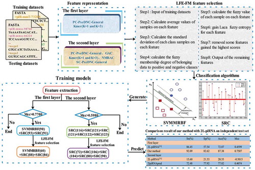
Table 5. Comparison results on the same training dataset to identify piRNAs via 5/10-fold validation on our training dataset and GA-WE balanced benchmark dataset.

Dataset	Method		Sn(%)	Sp(%)	Acc(%)	Mcc
Our training dataset 5-fold cross-validation	Accurate piRNA prediction		83.10	82.10	82.60	0.6510
	GA-WE		90.60	78.30	84.40	0.6940
	2 L-piRNA		88.30	83.90	86.10	0.7230
	2lpiRNApred		91.89	85.54	88.72	0.7759
GA-WE balanced benchmark dataset 10-fold cross-validation	Human	Piano	85.50	26.50	56.00	-
		k-mer^[Citation17]	85.59	76.40	81.20	-
		Accurate piRNA prediction^[Citation19]	81.50	80.00	80.70	-
		GA-WE^[Citation20]	85.80	82.00	83.90	-
		2lpiRNApred	92.70	90.10	91.40	0.8283
	Mouse	Piano^[Citation18]	83.70	23.60	53.65	-
		k-mer^[Citation17]	86.20	77.60	81.90	-
		Accurate piRNA prediction^[Citation19]	86.30	75.60	81.00	-
		GA-WE^[Citation20]	82.60	85.00	83.80	-
		2lpiRNApred	98.50	88.75	93.63	0.8767
	Drosophila	Piano^[Citation18]	83.60	54.70	69.20	-
		k-mer^[Citation17]	92.70	97.70	95.20	-
		Accurate piRNA prediction^[Citation19]	95.20	96.50	95.80	-
		GA-WE^[Citation20]	94.90	96.60	95.90	-
		2lpiRNApred	97.00	90.20	93.60	0.8740

lower than that by k-mer, accurate piRNA prediction, and GA-WE, the values of Sn were about 1.8%–4.3% higher in the GA-WE Drosophila balanced benchmark dataset. Based on 5/10- fold cross-validation results, it can be concluded that the predictive tool was greatly affected by the selected benchmark dataset. However, 2lpiRNApred exhibited better robustness and its obtained accuracy ranged from 2.62% to 39.98%.

As can be seen in Table 5, 2lpiRNApred obtained the best Sn of 98.5%, which generally led to 3.3% and 3.6% improvements with regard to the second best accurate piRNA prediction and third best GA-WE, respectively. In terms of another evaluation criterion, Sp, 2lpiRNApred obtained the best average Sp of 88.65%, GA-WE obtained the second best average Sp of 85.48%, while accurate piRNA prediction obtained the third best average Sp of 83.55%. We also compared 2lpiRNApred with 2 L-piRNA, which is currently the only computational method for identifying whether piRNAs function in inducing target mRNA deadenylation; the comparison results are shown in Table 6. The comparison results clearly show that 2lpiRNApred was better than 2 L-piRNA.

Table 6. Comparison results with 2 L-piRNA [21] via five-fold cross-validation on our training dataset.

Method	Sn (%)	Sp (%)	Acc (%)	Mcc
The first layer
2 L-piRNA^[Citation21]	88.30	83.90	86.10	0.7230
2lpiRNApred	91.89	85.54	88.72	0.7759
The second layer
2 L-piRNA^[Citation21]	79.10	76.00	77.60	0.5520
2lpiRNApred	82.37	77.57	79.97	0.6001

To further test and verify the performance of 2lpiRNApred, we also compared it with piRNN and 2 L-piRNA, which the web-server or github was available in our independent test dataset. As can be seen in Table 7, 2lpiRNApred remarkably outperformed piRNN and 2 L-piRNA, and the values of Mcc by 2lpiRNApred were about 0.4875 and 0.2908 higher than those by piRNN and 2 L-piRNA when identifying piRNAs in the first layer. 2lpiRNApred furthered comparison with 2 L-piRNA, which was only one computational method that identifies whether piRNAs function in inducting target mRNA deadenylation, and the value of Acc by 2lpiRNApred was about 56.47% higher than that by 2 L-piRNA. These results indicated that 2lpiRNApred represented a remarkable improvement not only in identifying piRNAs, but also in determining whether piRNAs function in inducting target mRNA deadenylation.

Figure 2. The prediction performance of each sub-classifier using proposed LFE-GM feature selection algorithm by five-fold cross-validation in layer I and II.

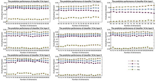
Table 7. A comparison of the proposed predictor with 2 L-piRNA and piRNN on our independent test dataset.

Method	Sn (%)	Sp (%)	Acc (%)	Mcc
First layer
piRNN(celegans)	87.21	48.15	67.79	0.3845
piRNN(Dmelanogaster)	95.89	23.54	59.91	0.2819
piRNN(Human)	94.37	30.15	62.43	0.3203
piRNN(Rat)	96.50	20.62	58.76	0.2632
2 L-piRNA^[Citation21]	86.45	57.54	72.07	0.4599
2lpiRNApred	92.09	82.62	87.38	0.7507
Second layer
piRNN	N/A	N/A	N/A	N/A
2 L-piRNA^[Citation21]	15.60	21.53	20.55	−0.5015
2lpiRNApred	72.48	77.92	77.02	0.4074

Note: N/A represented that corresponding methods failed to yield the results for the second layer prediction.

Considering the similarity of the training dataset can influence the prediction results, we further investigated the performance of CarSite-II by setting thresholds from 0.8 to 0.5 with CD-HIT program. We reported the values of Sn, Sp, Acc, and MCC obtained on different thresholds in Table 8. The results showed that the performance was not sensitive to the similarity of the training samples from 0.8 to 0.5.

Table 8. Testing results using the CD-HIT Program to redundancy on our training datasets via five-fold cross-validation.

Thresholds	Sn(%)	Sp(%)	Acc(%)	MCC
The first layer
0.5	90.92	87.01	88.86	0.7781
0.6	90.36	86.53	88.36	0.7682
0.7	90.34	86.48	88.34	0.7677
0.8	91.89	85.54	88.72	0.7759
The second layer
0.5	78.41	75.67	77.00	0.5406
0.6	77.69	75.76	76.67	0.5335
0.7	78.77	76.19	77.40	0.5484
0.8	82.37	77.57	79.97	0.6001

4. Conclusion

In this study, we proposed a novel feature selection algorithm, LFE-GM, to reduce the dimensionality of the features. Based on SRC and SVMMDRBF classifier algorithms and five feature extraction strategies (Kmer, PC, SC, NMBAC, and GAC), a two-layered integrated classifier algorithm, 2lpiRNApred, was constructed to identify piRNAs in the first layer and determine whether piRNAs function in inducing target mRNA deadenylation in the second layer. The main conclusions of this study are summarized as follows:

• The proposed LFE-GM feature selection algorithm can reduce the dimensionality of the features with a high efficiency and accuracy.

• According to the comprehensive performance of the two-layered integrated classifier algorithm, 2lpiRNApred, in this study, integration of SRC and SVMMDRBF classifier algorithms is perfectly tailored to identify piRNAs and determine whether piRNAs function in inducing target mRNA deadenylation, consequently obtaining satisfactory prediction results.

• The proposed LFE-GM feature selection strategy in the feature selection module is proved to be an effective scenario to improve the performance of the proposed integrated algorithm.

• The proposed 2lpiRNApred model solves the classification problem with three classes (class 1: piRNA involved in deadenylation, class 2: piRNA not involved in deadenylation, class 3: not a piRNA) with binary classifiers.

Availability and implementation

http://lab.malab.cn/soft/pirna/

https://github.com/JianyuanLin/2lpiRNApred

Disclosure of potential conflicts of interest

No potential conflicts of interest were disclosed.

Supplementary material

Supplementary data for this article can be accessed here.

Additional information

Funding

This work was supported by Natural Science Foundation of Fujian Province[2017J01099]; the national key R&D program of China [2017YFE0130600]; Project of marine economic innovation and development in Xiamen [16PFW034SF02]; President Fund of Xiamen University [20720170054]; the Natural Science Foundation of China [61772441,61472335,61922020,61425002,61872007].

Notes on contributors

Yun Zuo

Yun Zuo received the bachelor’s degree from Liaocheng University in 2015 and received the master’s degree from Dalian Maritime University with the Department of Mathematics in 2018. Currently, she is pursuing the Ph.D. degree in Department of Computer Science, Xiamen University. Her research is in the areas of bioinformatics and machine learning. Several related works have been published by Bioinformatics, Molecular BioSystems, Journal of Theoretical Biology etc.

Quan Zou

Quan Zou (M’13-SM’17) received the BSc, MSc and the PhD degrees in computer science from Harbin Institute of Technology, China, in 2004, 2007 and 2009, respectively. He worked in Xiamen University and Tianjin University from 2009 to 2018 as an assistant professor, associate professor and professor. He is currently a professor in the Institute of Fundamental and Frontier Sciences, University of Electronic Science and Technology of China. His research is in the areas of bioinformatics, machine learning and parallel computing. Several related works have been published by Science, Briefings in Bioinformatics, Bioinformatics, IEEE/ACM Transactions on Computational Biology and Bioinformatics, etc. Google scholar showed that his more than 100 papers have been cited more than 5000 times. He is the editor-in-chief of Current Bioinformatics, associate editor of IEEE Access, and the editor board member of Computers in Biology and Medicine, Genes, Scientific Reports, etc. He was selected as one of the Clarivate Analytics Highly Cited Researchers in 2018.

Jianyuan Lin

Jianyuan Lin graduated from Hangzhou University of electronic science and technology with a major in computer science and technology in 2017. He is currently studying for a master’s degree at Xiamen University. His current research interests include artificial intelligence, data mining, machine learning, and deep learning.

Min Jiang

Min Jiang received the bachelor’s and Ph.D. degrees in computer science from Wuhan University, Wuhan, China, in 2001 and 2007, respectively. He was a Post-Doctoral Research Fellow with the Department of Mathematics, Xiamen University, Xiamen, China, where he is currently a full Professor with the Department of Cognitive Science and Technology. His current research interests include machine learning, computational intelligence, neural-symbolic integration, dynamic multiobjective optimization, machine learning, software development, and basic theories of robotics.

Xiangrong Liu

Xiangrong Liu received his Ph.D. degree in control science and engineering from Huazhong University of Science and Technology at Wuhan, China in 2007. He finished his postdoctoral training in the school of Electronics Engineering and Computer Science at Peking University from 2007 to 2009. In 2009 he joined Xiamen University and is currently a professor in Department of Computer Science, Xiamen University. His research focuses on computational intelligence and bioinformatics.

References

- Claverie JM. Fewer genes, more noncoding RNA. Science. 2005;309(5740):1529.
- Mattick JS. The functional genomics of noncoding RNA. Science. 2005;309(5740):1527–1528.
- Aravin A, Gaidatzis D, Pfeffer S, et al. A novel class of small RNAs bind to MILI protein in mouse testes. Nature. 2006 Jul;442(7099):203–207.
- Lau NC, et al. Characterization of the piRNA complex from rat testes. Science. 2006 Jul;313(5785):363–367.
- Grivna ST, et al. A novel class of small RNAs in mouse spermatogenic cells. Gene Dev. 2006 Jul;20(13):1709–1714.
- Meenakshisundaram H. Existence of snoRNA, microRNA, piRNA characteristics in a novel non-coding RNA: x-ncRNA and its biological implication in homo sapiens. Washington D. 2009 Jan;1(2):31–40.
- Seto AG, Kingston RE, Lau NC, et al. The coming of age for piwi proteins. Mol Cell. 2007 Jun;26(5):603–609.
- Ruby JG, Jan C, Player C, et al. Large-scale sequencing reveals 21U-RNAs and additional microRNAs and endogenous siRNAs in C. elegans. Cell. 2006 Dec;127(6):1193–1207.
- Cox DN, Chao A, Baker J, et al. A novel class of evolutionarily conserved genes defined by piwi are essential for stem cell self-renewal. Gene Dev. 1998 Dec;12(23):3715–3727.
- Klattenhoff CA, Theurkauf W, et al. Biogenesis and germline functions of piRNAs. Development. 2008;135(1):3–9.
- Brennecke J, Aravin AA, Stark A, et al. Discrete small RNA-generating loci as master regulators of transposon activity in drosophila. Cell. 2007 Mar;128(6):1089–1103.
- Thomson T, Lin H, et al. The biogenesis and function of PIWI proteins and piRNAs: progress and prospect. Annu Rev Cell Dev Bi. 2009;25:355–376.
- Houwing S, Kamminga LM, Berezikov E, et al. A role for piwi and piRNAs in germ cell maintenance and transposon silencing in Zebrafish. Cell. 2007 Apr;129(1):69–82.
- Lu Y, Li C, Zhang K, et al. Identification of piRNAs in HeLa cells by massive parallel sequencing. Bmb Rep. 2010 Sep;43(9):635–641.
- Cheng J, Guo J-M, Xiao B-X, et al. piRNA, the new non-coding RNA, is aberrantly expressed in human cancer cells. Clin chim acta. 2011 Aug;412(17–18):1621–1625.
- Huang G, Hu H, Xue X, et al. Altered expression of piRNAs and their relation with clinicopathologic features of breast cancer. Clin Transl Oncol. 2013 Jul;15(7):563–568.
- Zhang Y, Wang X, Kang L, et al. A k-mer scheme to predict piRNAs and characterize locust piRNAs. Bioinformatics. 2011 Mar;27(6):771–776.
- Wang K, Liang C, Liu J, et al. Prediction of piRNAs using transposon interaction and a support vector machine. BMC Bioinformatics. 2014;15:419.
- Luo L, Li D, Zhang W, et al. Accurate prediction of transposon-derived piRNAs by integrating various sequential and physicochemical features. Plos One. 2016 Apr;11(4):e0153268.
- Li D, Luo L, Zhang W, et al. A genetic algorithm-based weighted ensemble method for predicting transposon-derived piRNAs. BMC Bioinformatics. 2016;17:329.
- Liu B, Yang F, Chou K-C, et al. 2L-piRNA: A two-layer ensemble classifier for identifying piwi-interacting RNAs and their function. Mol Ther-Nucl Acids. 2017;7:267–277.
- Wang K, Hoeksema J, Liang C, et al. piRNN: deep learning algorithm for piRNA prediction. Peerj. 2018;6:e5429.
- Bu D, Yu K, Sun S, et al. NONCODE v3. 0: integrative annotation of long noncoding RNAs. Nucleic Acids Res. 2012 Jan;40(D1):D210–D215.
- Zhang P, et al. piRBase: a web resource assisting piRNA functional study. Database-Oxford, no. bau110. 2014 Nov.
- Huang Y, Niu B, Gao Y, et al. CD-HIT suite: a web server for clustering and comparing biological sequences. Bioinformatics. 2010 Mar;26(5):680–682.
- Jia CZ, Zuo Y, et al. S-SulfPred: a sensitive predictor to capture S-sulfenylation sites based on a resampling one-sided selection undersampling-synthetic minority oversampling technique. J Theor Biol. 2017;422:84–89.
- Wu H-Y, Lu C-T, Kao H-J, et al. Characterization and identification of protein O-GlcNAcylation sites with substrate specificity. BMC Bioinformatics. 2014;15:S1.
- Shao J, Xu D, Tsai S-N, et al. Computational identification of protein methylation sites through Bi-profile bayes feature extraction. Plos One. 2009;4:e4920.
- Xie D, Li A, Wang M, et al. LOCSVMPSI: a web server for subcellular localization of eukaryotic proteins using SVM and profile of PSI-BLAST. Nucleic Acids Res. 2005 Jul;33(Web Server):W105–W110.
- Jones DT. Protein secondary structure prediction based on position-specific scoring matrices. J Mol Biol. 1999;292(2):195–202.
- Liu B, Liu, F., Wang, X, et al. Pse-in-one: a web server for generating various modes of pseudo components of DNA, RNA, and protein sequences. Nucleic Acids Res. 2015 Jul;43(W1):W65–W71.
- Liu B, Wu H, Chou K-C, et al. Pse-in-one 2.0: an improved package of web servers for generating various modes of pseudo components of DNA, RNA, and protein sequences. Nat Sci. 2017;9:67–91.
- Lee D, Karchin R, Beer MA, et al. Discriminative prediction of mammalian enhancers from DNA sequence. Genome Res. 2011 Dec;21(12):2167–2180.
- Noble WS, Kuehn S, Thurman R, et al. Predicting the in vivo signature of human gene regulatory sequences. Bioinformatics. 2005 Jun;21(1):I338–I343.
- Gupta S, Dennis J, Thurman RE, et al. Predicting human nucleosome occupancy from primary sequence. Plos Comput Biol. 2008;4:e1000134.
- Chen W, Zhang X, Brooker J, et al. PseKNC-general: a cross-platform package for generating various modes of pseudo nucleotide compositions. Bioinformatics. 2015 Jan;31(1):119–120.
- Feng Z-P, Zhang C-T, et al. Prediction of membrane protein types based on the hydrophobic index of amino acids. J Protein Chem. 2000 May;19(4):269–275.
- Sokal RR, Thomson BA, et al. Population structure inferred by local spatial autocorrelation: an example from an Amerindian tribal population. Am J Phys Anthropol. 2006 Jan;129(1):121–131.
- Wright J, et al. Demo: robust face recognition via sparse representation. Ieee Fg. 2008;1-2:942–943.
- Wright J, Ma Y, Mairal J, et al. Sparse representation for computer vision and pattern recognition. P Ieee. 2010 Jun;98(6):1031–1044.
- Deng W, Hu J, Guo J, et al. Extended SRC: undersampled face recognition via intraclass variant dictionary. IEEE T Pattern Anal. 2012 Sep;34(9):1864–1870.
- Yang J, Zhang L, Xu Y, et al. Beyond sparsity: the role of L1-optimizer in pattern classification. Pattern Recognition. 2012 Mar;45(3):1104–1118.
- Guo S, et al. Similarity weighted sparse representation for classification. ICPR, pp. 1241–1244, Nov. 2012.
- Lu CY, Min H, Gui J, et al. Face recognition via weighted sparse representation. J Vis Commun Image R. 2013 Feb;24(2):111–116.
- Li CG, et al. Local sparse representation based classification. IEEE, no. 11580253, Aug 2010.
- Mei JY, Liu M, Karimi HR, et al. LogDet divergence-based metric learning with triplet constraints and its applications. IEEE T Image Process. 2014 Nov;23(11):4920–4931.
- Mei JY, Liu M, Wang Y-F, et al. Learning a mahalanobis distance-based dynamic time warping measure for multivariate time series classification. IEEE T Cybern. 2016 Jun;46(6):1363–1374.
- Zuo Y, Jia C, Li T, et al. Identification of cancerlectins by split Bi-profile bayes feature extraction. Curr Proteomics. 2018;15(3):196–200.
- Tung CW. Prediction of pupylation sites using the composition of k-spaced amino acid pairs. J Theor Biol. 2013 Nov;336(25):11–17.
- Hosseinzadeh M, et al. Using fuzzy undersampling and fuzzy PCA to improve imbalanced classification through rotation forest algorithm. CSSE. Aug 2015.
- Jia CZ, Zuo Y, Zou Q, et al. O-GlcNAcPRED-II: an integrated classification algorithm for identifying O-GlcNAcylation sites based on fuzzy undersampling and a k-means PCA oversampling technique. Bioinformatics. 2018 Jun;34(12):2029–2036.
- Luca AD, Termini S, et al. A definition of a nonprobabilistic entropy in the setting of fuzzy sets theory. Inf Control. 1972;20(4):301–312.