Machine learning based renewable energy generation and energy consumption forecasting

ABSTRACT

Renewable energy generation sources are the need of the hour to mitigate the challenges of fossil fuels, environmental impacts, large transmission and distribution losses, and variable consumption pattern. Renewable energy such as solar PV generation or wind generation is most unpredicted generation and depends upon weather constraints. A promising prediction of generation is a suitable solution for this problem. A machine learning-based conventional neural network algorithm is proposed to forecast the generation and calculate the errors in generation forecast. The generated energy is supplied to consumers, but the consumers consume electricity by their choice and an energy management model is required at the consumer end to supply the available predicted generation to develop a self-sustainable microgrid. The energy consumption at consumer end is essential to predict, and based on the predicted consumption at hourly bases, the cost model for the consumers is developed. The consumption profile is forecasted using long short-term memory as it is a good tool for time-series forecasting using available sequential load consumption data. The demand is forecasted and analyzed for selected load categories (i.e. fixed, non-shift-able, and shift-able loads). The evaluation matrix mean square error (MSE), mean absolute error, and root mean square error (RMSE) are used for the error calculations. The RMSE for solar and wind power generation forecasting have been 2.472 and 3.034, respectively. The RMSE for fixed, non-shiftable, and shiftable demand forecasting have been 0.027, 0.067, and 0.21, respectively. The results show that the proposed methods for predictions of solar, wind power generation and energy consumption forecast achieve better accuracy. The presented methodology can be implemented with energy storage for renewable energy production and demand management for energy from sustainable energy resources.

KEYWORDS:

• Renewable energy forecasting
• Energy demand forecasting
• Solar energy forecasting
• Wind energy forecasting
• Machine learning

Introduction

The global economy is expanding quickly, raising living standards and driving up energy consumption, but fossil fuel supplies are becoming less viable (Talwariya et al. 2022). Global climate change and sustainable development are the two key concerns with regard to energy production. The production of all energy is mostly reliant on natural gas, coal, and oil, and annual energy consumption rises by 2% (Wang et al. 2019). Anthropogenic greenhouse gas emissions are significantly increased by the extensive use of fossil fuels, which leads to climatic anomalies including droughts and heavy rainfall. If the predicted energy is supplied through fossil fuels, greenhouse gas emissions are predicted to rise by 30% over the next 20 years (Ghaderi, Sanandaji, and Ghaderi 2017; Nam, Hwangbo, and Yoo 2020). This increased emission has the most negative impact on the environment and the health of living things (Gard-Murray 2022; Zhang et al. 2022).

Therefore, due to the challenges of generating electricity using fossil fuels, renewable energy sources (RES) are widely investigated and promoted by governments, scientists, and industrial professionals. RES includes solar photovoltaic, wind turbines, hydropower plants, tidal power plants, etc. Hydropower plants are the most dependable out of these RES, but the generation takes place at a remote location, which increases transmission and distribution losses. Out of the remaining RES, solar PV and wind turbines are widely used at load centers for energy generation throughout the world (Baldi et al. 2018; Carley et al. 2017; Johannesen, Kolhe, and Goodwin 2022). These energy sources depend upon weather constraints to generate electricity and are highly uncertain, and their high volatility poses a big challenge to the stable operation and economic dispatch of the power system (Ahmad et al. 2018; Zhang et al. 2022).

A suitable solution may be provided by predicting the generation from RES a day ahead or in real time and then supplying it to consumers. The literature review on prediction of generation has been performed using a physical model, a statistical model, a machine learning model, etc. (Li et al. 2021).

Physical models do not require past generation data, but they predict generation based on a physical model that takes into account weather constraints such as solar radiation, wind speed, temperature, incident angle, and efficiency. It is complicated for physical models to provide the required weather constraints, and they offer poor interference and computational complexity. Unlike the physical model, the statistical model maps the relation between past generation data and predicted time-series data using linear fitting (for example, regression analysis, autoregressive models, etc.), which makes it difficult to fit strong fluctuations and the high dimensionality of RES (Agrawal et al. 2022; Mathew and Kolhe 2022; Singh, Talwariya, and Kolhe 2019b).

Machine learning models are roughly classified as shallow learning models and deep learning models. Shallow learning models are mainly designed to extract nonlinear features for smaller networks, e.g. k-nearest neighbor, back propagation, support vector regression, etc. However, as big data technology and intelligence optimization theories have advanced recently, shallow learning models will be vulnerable to the dimensionality and under-fitting curse, making it difficult to forecast RES generation data in a big data era. Deep learning models are the most promising and offer more accurate results for data extraction when big data are applicable, e.g., deep neural networks (DNNs), recurrent neural networks (RNNs), long short-term memory (LSTM) models, and conventional neural networks (CNNs). The forecasting of the generation from RES depends not only on the selection of a suitable model but also on the selection of hyperparameters and network structure. Based on the application and available data, a suitable model is selected for the generation forecast. The CNN offers time-series forecasting for the generation from RES, which is variable with respect to time. Therefore, this model is utilized for the prediction of generation (Talwariya et al. 2018; Talwariya, Singh, and Kolhe 2021; Wang et al. 2020).

Once the generation forecasting data are available, we need to supply continuous energy to the consumers, but the energy consumption profile of each consumer is random. Every consumer has their own way to utilize energy, and it is also unpredictable. Forecasting consumption is critical for keeping consumption in line with the available predicted generation. Loading a large number of consumers’ historical consumption data and forecasting their generation is another difficult task for physical models, statistical models, and shallow machine learning models. Therefore, consumption forecasting is done using deep learning models based on hyperparameter tuning and network structure. The options available are RNN, CNN, DNN, and LSTM. RNN and CNN models carry forward irrelevant information and slow down the model in the case of large number of consumers. The LSTM is also a type of RNN with higher memory power. This model is selected for consumption forecasting and to manage demand at the consumer end. Connected appliances are categorized as shiftable, non-shiftable, and fixed appliances. Lights, refrigerators, and other stationary appliances work exclusively during predetermined times and for predetermined durations, known as fixed appliances. Heaters, air conditioners, dishwashing machines, and other non-shiftable appliances have fixed durations but variable time slots that allow consumers to transfer their use from one duration to another. The duration and time slot of shiftable appliances, such as central cooling systems and electric automobiles, are both programmable. Since the energy usage of all this equipment is unpredictable, consumers’ energy management needs to be reliable (Liu et al. 2021; Malakouti et al. 2022). The major contributions of the paper are summarized:

• Forecast the solar and wind power generation, which depends upon weather constraints.

• Forecast the energy consumption by categorizing the appliances in fixed, non-shiftable and shiftable loads.

• Calculate the different errors to measure the accuracy of the deep learning model.

• Manage the energy demand for making self-sustainable grid with renewable energy sources.

The paper is organized as follows: the proposed solar-wind forecasting model using CNN is discussed in Section 2. Energy consumption prediction using LSTM model is discussed in Section 3. Results and conclusion of the work with future scope are discussed in Sections 4 and 5, respectively.

Proposed solar-wind energy forecast model

Solar and wind energy resources are the most growing energy generation sources and can be suitable alternatives for the fossil fuels with appropriate energy management. The renewable energy prediction as well as the demand predictions are essential for the demand side management, and the machine learning tools can be used for predictions as well as energy management. The renewable energy generation and load datasets are required for doing the forecasting through machine learning tools. The available datasets need pre-processing for effective utilization, which involves importing the dataset, removing abnormal data, overcoming the missing data, data normalization. and initializing parameters. Performance-based predictions from wind and solar energy systems using k-nearest neighbor (kNN) algorithm is presented in (Mathew and Kolhe 2022). The CNN is most popularly used tool for predictions using some data patterns. The solar prediction framework using echo state network with CNN is explained in (Khan et al. 2022) and based on that the CNN model primary framework is illustrated in Figure 1. In this work, the CNN is used for predictions and the processed datasets are used in multiple hidden layer CNN model. In this model N convolutional hidden layers are used. The output layer of the CNN is considered for forecasting solar and wind energy generation. After getting the predicted output, CNN helps in visualizing and interpreting the data with some patterns. It can compare the results with actual generation and identify the accuracy of the model. If the output results are not satisfactory, then it fine tunes the hyperparameters and again processes the obtained results for more accuracy analysis.

Figure 1. Solar wind generation forecasting using CNN.

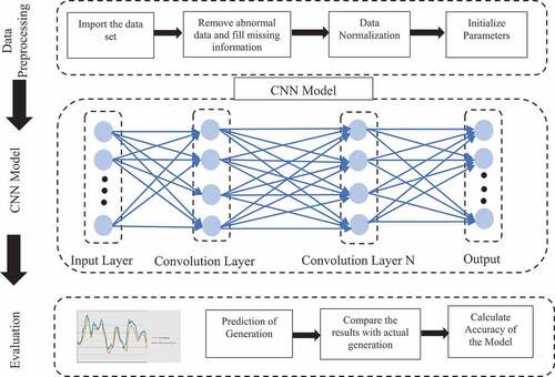
Specialized neural networks such as CNN are specifically designed to extract locally specific (spatial) data from the input data. CNN can do this by explicitly encoding it in the design. A standard CNN is made up of three different types of layers (or “building blocks”): convolution, pooling, and fully linked layers. Feature extraction is carried out using convolution and pooling layers in layers one and two and it is mapped into the output by a fully connected layer.

Historical solar and wind energy generation data on a single time scale have a limited quantity of time information and cannot accurately capture the trend and time sequence information. The original solar and wind power data must therefore be processed to extract more time sequence information. Some useful properties can be effectively extracted by convolutional neural networks. Therefore, in order to extract various time sequence properties from the original solar wind power generation data, this article uses a convolutional neural network. Using two-dimensional convolution, the initial solar wind energy generation sequence is transformed into a solar-wind energy sequence at various scales and mathematically written in eq. 1:

(1) $X_{\mathit{i}(\mathit{t})}=\mathit{Conv}2\mathit{d}(G_{\mathit{input}})$(1)

where $X_{\mathit{i}\left(\mathit{t}\right)}$is the sequence of solar-wind power generated by convolution at different time scales and $G_{\mathit{input}}$is the historical solar and wind power generation data. To extract the characteristics of various time scales, two-dimensional convolutions with convolution kernel sizes of $15\times 1,30\times 1,60\times 1,90\times 1,$and$120\times 1$ are used. The original solar and wind power generation sequences are split into five sub-sequences with time scales of 15, 30, 60, 90, and 120 min using five convolution kernels.

The output of the preceding layers is convolved using a convolution kernel in a convolutional layer to create an output feature vector $\mathit{X}$, which may contain several feature vector convolutions. If the sequence of wind and solar energy generation is $X_{\mathit{i}\left(\mathit{t}\right)}=X_{1\left(\mathit{t}\right)},X_{2\left(\mathit{t}\right)},X_{3\left(\mathit{t}\right)},X_{5\left(\mathit{t}\right)}$ in five sub-sequences with time scales. The mathematical operation of first convolution layer can be written as eq. (2):

(2) $y_i^1=\mathit{\sigma }\left(\left({\sum }_{m=1}^M{\sum }_{i=1}^5{W}_m^1{X}_{i(t)}^1\right)+b_i^1\right)$(2)

where $y_i^1$is the output of the first convolutional layer, $W_m^1$ is the weight matrix for first convolutional layer, and $\mathit{m}$ indicates the filter index value. $b_i^1$ is the bias in the convolution layer for different time sequences and $\mathit{\sigma }$ is sigmoid function selected for the first convolution layer. Similarly, the output of the second convolutional layer is mathematically written as eq. (3)

(3) $y_i^2=\mathit{\sigma }\left(\left({\sum }_{m=1}^M{\sum }_{i=1}^5{W}_m^2{X}_{i(t)}^2\mathit{\hspace{0.17em}}\right)+b_i^2\right)$(3)

Similarly, $n^{\mathit{th}}$ convolutional layer is also written as eq. (4), where activation function ReLU is used to rectify the output of previous layers written as eq. (5).

(4) $y_i^n=\mathit{\varsigma }\left(\left({\sum }_{m=1}^M{\sum }_{i=1}^5{W}_m^n{X}_{i\left(t\right)}^n\right)+b_i^n\right)$(4)

(5) $\mathit{f}\left(X_{\mathit{i}\left(\mathit{t}\right)}\right)=max\left(0,X_{\mathit{i}\left(\mathit{t}\right)}\right)$(5)

The activation function ReLU provides only positive output and trapped negative output by converting into zero. Based on the predicted generation, price is forecast and communicated to consumers for managing the consumption at consumer end.

Deamnd Consumption Model

Based on the energy generation, which is predicted using CNN model of machine learning, the consumption is managed at consumer end. At the consumer end, all linked loads are divided into three basic types of loads. The load stays on until the specified task is completed once it has begun. In this scenario, each client should choose a scheduling time to run their shiftable load, $a_s$. The problem’s objective purpose is described in (6).

(6) $\mathit{Min}\mathit{\hspace{0.17em}}\mathit{obj}\mathit{\hspace{0.17em}}={\sum }_{a_s=1}^{a_{\mathit{s},\mathit{i}}}{\sum }_{t=t_{s,a_s}}^{t_{d,a_s}}((P_{a_s\mathit{\hspace{0.17em}}}(\mathrm{t}))(\mathit{\rho }(\mathit{t})))$(6)

where $P_{a_s\mathit{\hspace{0.17em}}}\left(\mathit{t}\right)$ is the real power consumption of shiftable load a_s for the particular time duration denoted by t. The time of shiftable load consuming electricity is from the starting time denoted as $t_{s,a_s}$ and the time till this shiftable load is in operation is denoted as $t_{d,a_s}$. ϼ(t) is the proposed energy consumption price for particular duration given based on the forecast model for time interval t which is calculated by (7).

(7) $\mathit{\rho }(\mathit{t})\mathit{\hspace{0.17em}}=f_s\left({\sum }_{i=1}^n(P_{{\mathit{a}}_{\mathit{sn}}\mathit{\hspace{0.17em}}}(\mathit{t})+\mathit{\hspace{0.17em}}{\sum }_{a_s=1}^{a_{\mathit{s},\mathit{i}}}{P}_{a_s\mathit{\hspace{0.17em}}}(\mathit{t})\mathit{\hspace{0.17em}})+P_l(\mathit{t})\right)\mathit{\hspace{0.17em}}$(7)

where $P_{{\mathit{a}}_{\mathit{sn}}\mathit{\hspace{0.17em}}}\left(\mathit{t}\right)$ is the real power consumed by non-shiftable load for a particular duration t, and $P_l\left(\mathit{t}\right)$ denotes the total power losses at consumer end for particular time duration t for $i^{\mathit{th}}$ consumer. $f_s$ is the function for demand price forecast by utility based on the generation forecast.

Consumers are attempting to change shiftable loads scheduling durations to low-cost durations in order to reap the benefits. The appliance’s operating time is determined by (8).

(8) $t_{s,a_s}<\mathit{\hspace{0.17em}}\mathit{t}\mathit{\hspace{0.17em}}<t_{d,a_e}\mathrm{\forall }{a}_s,$(8)

A maximum allowable limit is set of each consumer denoted as $S_{\mathit{m},\mathit{i}}$ to reduce the chances of generating peak at low price duration for i^th consumer. Therefore, the total electricity consumed by $i^{\mathit{th}}$ consumer is denoted by (9). This total electricity consumed is also considered the reactive power consumption by unshiftable and shiftable loads are denoted as $Q_{{\mathit{a}}_{\mathit{sn}}\mathit{\hspace{0.17em}}}\left(\mathit{t}\right)$ and $Q_{a_s\mathit{\hspace{0.17em}}}\left(\mathit{t}\right)$, respectively, for the $i^{\mathit{th}}$ consumer.

(9) $(P_{{\mathit{a}}_{\mathit{sn}}}\left(\mathit{t}\right)+{\sum }_{a_s=1}^{a_{\mathit{s},\mathit{i}}}{P}_{a_s}\left(\mathit{t}\right){)}^2+(Q_{{\mathit{a}}_{\mathit{sn}}}\left(\mathit{t}\right)+{\sum }_{a_s=1}^{a_{\mathit{s},\mathit{i}}}{Q}_{a_s}\left(\mathit{t}\right){)}^2\le S_{m,i}^2\mathrm{\forall t}$(9)

The total power consumed by all shiftable and non-shiftable load is given by (10).

(10) $S_{\mathit{total}}(\mathit{t})\mathit{\hspace{0.17em}}=\mathit{\hspace{0.17em}}(f_s\left({\sum }_{i=1}^n(P_{{\mathit{a}}_{\mathit{sn}}\mathit{\hspace{0.17em}}}(\mathit{t})+\mathit{\hspace{0.17em}}{\sum }_{a_s=1}^{a_{\mathit{s},\mathit{i}}}{P}_{a_s\mathit{\hspace{0.17em}}}(\mathit{t})\mathit{\hspace{0.17em}})+P_l(\mathit{t})\right)\mathit{\hspace{0.17em}}+\mathit{\hspace{0.17em}}{f}_s\left({\sum }_{i=1}^n{Q}_{{\mathit{a}}_{\mathit{sn}}\mathit{\hspace{0.17em}}}(\mathit{t})+\mathit{\hspace{0.17em}}{\sum }_{a_s=1}^{a_{\mathit{s},\mathit{i}}}{Q}_{a_s\mathit{\hspace{0.17em}}}(\mathit{t})+Q_l(\mathit{t})\mathit{\hspace{0.17em}}\right)$(10)

where $Q_l\left(\mathit{t}\right)$ is the total reactive power losses at consumer end for particular time duration t for i^th consumer.

Machine learning model for energy consumption

Energy management

Electrical energy is distributed to users with variable characteristics, such as consumption levels, on a grid, which is a secure location. A more intelligent grid with appropriate energy management (distribution) systems reduces energy loss and depletion. Traditional systems offer all users electricity for free without considering their usage, the effects of climate change, or any of the other variables that contribute to inefficient energy use (Talwariya and Singh 2018). On the other hand, a smart grid keeps track of energy demands and distributes it appropriately. Grids typically perform badly due to their overload or, more significantly, the loss of energy demand data. There is no system in place to identify anomalous energy demand in the residential or business sectors as a result. This paper’s strategy uses an intermediate cloud analysis model to tackle this issue, where customer demands go through a number of analysis steps before being sent to smart grids. In the hypothetical energy management scenario shown in Figure 2, which makes use of the infrastructure we’ve suggested, future load forecasting is progressed to demand transmission and energy purchase for home consumers. To distinguish between each domestic consumer, the figure is colored differently.

Figure 2. Energy management model for domestic consumers using cloud.

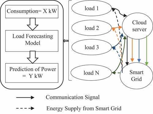
In Figure 2, a dotted line represents energy supply from the smart grid to different appliances at consumer end and the solid line represents communication signal between smart grid and intelligent electronic loads (which are able to communicate with smart grid) through cloud. The energy consumption for the following hour is produced by our recommended trained model using the energy data used in a minute by domestic consumers as input. Domestic users have a device with limited resources that includes a trained forecasting model. It uses historical data on energy use ($\mathit{X}\mathit{\hspace{0.17em}}\mathit{kW}$) as input and trains a model to forecast hourly energy use ($\mathit{Y}\mathit{\hspace{0.17em}}\mathit{kW}$). The request is made by domestic users and is sent to a cloud server, which saves it and examines it for anomalies by comparing it to previous demand data before delivering it to the smart grid. A abrupt shift in demand from a commercial or residential structure could be the anomaly. In response to the request, the smart grid delivers $\mathit{Y}\mathit{\hspace{0.17em}}\mathit{kW}$ of energy (Johannesen, Kolhe, and Goodwin 2019a; Talwariya and Singh 2018).

Future energy prediction

The technological contributions of our technique include future energy consumption prediction using a resource-constrained device with a decreased error rate and enhanced calculation. Before it can be applied to the model, the real-time data are pre-processed by the various steps. The first step in our novel sequential learning approach, which we describe below, is pre-processing raw data from an existing dataset in order to produce the best trained model.

Data pre-processing

Electric energy data include time, date, active and reactive power, current, voltage, and other elements that are involved in data collection via smart meters. The smart meter serves as hub, connecting the cables from numerous equipment or appliances on a single main board. Long-range parameters, redundancy, missing values, and other issues are common in the raw data, which is often collected for a month or a year (Mathew and Kolhe 2022) and they need to be pre-processed for renewable energy and load predictions considering the impact of external parameters (Johannesen, Kolhe, and Goodwin 2019a, 2022). These inaccuracies are a result of metering problems, individual faults, measurement device flaws, and environmental changes (Singh, Talwariya, and Kolhe ; Talwariya et al. 2020; Talwariya, Singh, and Kolhe 2019). As a result, techniques for data normalization and purification are needed for electric energy data in order to get more refinement and acceptable results (Johannesen, Kolhe, and Goodwin 2021; Talwariya, Singh, and Kolhe 2022).

Employ a variety of pre-processing techniques in our framework to clean the data before using it for training. In order to extract the pertinent data, we first remove the missing values (Singh, Talwariya, and Kolhe ; Talwariya et al. 2020). We do outlier identification before using the normalizing process. It has the benefit of avoiding odd numbers that are unusual or out of the ordinary, which can change the range of normalization values and push the parameters closer to the maximum/minimum range. The crucial pre-processing step of normalization came next, and we explored many options before settling on the optimal “standard transform selection” for the final research. Examples of normalization strategies include the Min-max scalar, the standard-scalar, the Max-Abs scalar, the quantile transform, etc. Data following normalization for domestic parameters, where data in the range of $0$–$250$ is normalized between $-2.5$ and $3.5$, has a transitional effect. It can be helpful to train precise models because most parameters lie between $-1$ and $1$. Finally, we compress the original datasets (domestic or commercial) in short intervals because we are dealing with short-term energy consumption forecasts. Pre-processing techniques over raw data boost the prediction and performance of the machine learning algorithm.

Load forecasting model

RNN operates on numerous inputs at once as opposed to the single input at a time employed by conventional energy prediction models. RNN is a neural network that feeds forward and has internal memory. Every input receives the same function, and the output depends on the prior prediction. This paper employed LSTM, which contain three gates input, forget, and output, to learn long-term sequences, to solve the RNN model, and to forget the effect for long-sequence problem. Calculations for the input, forget, and output gates are given by (11)–(13), respectively.

(11) $i_g=\mathit{\sigma }[w_{i_g}[h_{\mathit{g}-1,}{x}_g]+b_{i_g}]$(11)

(12) $f_g=\mathit{\sigma }[w_{f_g}[h_{\mathit{g}-1,}{x}_g]+b_{f_g}]$(12)

(13) $o_g=\mathit{tanh}[w_{o_g}[h_{\mathit{g}-1,}{x}_g]+b_{o_g}]$(13)

where $i_g$ stands for the input gate equation, $f_g$ for the forget gate equation, and $o_g$ for the relationship of the output gate. To convert the provided data to gates in the range of $0$–$1$, the sigmoid activation function is used for the input and forget gate and tangent is utilized for the output gate. The weights of the input, forget, and output gates are $w_{i_g},w_{f_g}$, and $w_{o_g}$, respectively. The input for the existing gate is $x_g$, while the output of the previous gate is indicated by $h_{\mathit{g}-1}$. These gates also include biased terms, denoted by $b_{i_g},b_{f_g},\mathit{\hspace{0.17em}}$and $b_{o_g}$, respectively, for input, forget, and output gate, respectively.

Results and discussion

Error calculation in model

Mean-square-error (MSE), root-mean-square-error (RMSE), and mean-absolute-error (MAE) are used to assess the performance of the prediction models (Johannesen, Kolhe, and Goodwin 2019b). The first widely used metric is MSE, which measures the mean-squared difference between expected and actual values, or the average of squared errors, as given in (14).

(14) $\mathit{MSE}=\mathit{\hspace{0.17em}}\frac{1}{n}{\sum }_1^n(Y_{\mathit{act}}-\mathit{\hspace{0.17em}}{Y}_{\mathit{pre}}{)}^2$(14)

In forecasting, climatology, and regression analysis, the standard deviation of prediction errors (RMSE) is a commonly used statistic that is used to validate experimental models that are calculated using (15).

(15) $\mathit{RMSE}=\sqrt{\frac{1}{n}{\sum }_1^n{({\mathit{Y}}_{\mathit{act}}-Y_{\mathit{pre}})}^2}$(15)

MAE, or the average magnitude of the prediction errors, measures the size of the errors without accounting for their direction. The average of all the absolute differences between a model’s forecast and its actual values over all instances in the testing set is what it is, to put it another way. The mathematical formula for MAE computation is shown in (16).

(16) $\mathit{MAE}=\mathit{\hspace{0.17em}}\frac{1}{n}{\sum }_1^n|Y_{\mathit{act}}-\mathit{\hspace{0.17em}}{Y}_{\mathit{pre}}|$(16)

where in (14), (15), and (16), $Y_{\mathit{pre}}$ is the anticipated consumption made by the CNN and LSTM model for generation and consumption forecast, respectively, while $Y_{\mathit{act}}$ represents the consumers’ actual consumption.

Solar-wind energy generation forecast model

A solar and wind farm is considered for the prediction of generation; maximum capacity of solar power generation is 60 kW and maximum wind capacity is $40\mathit{kW}$ at typical location in Rajasthan. Overall capacity of the plant is $100\mathit{kW}$. For the prediction of historical data of generation, humidity, temperature, wind speed, solar radiation, wind direction, rainfall, etc. are provided as input and using the proposed CNN model energy forecast for a typical day is shown in Figures 3 and 4, respectively, for solar and wind power generation.

Figure 3. Solar power generation curve.

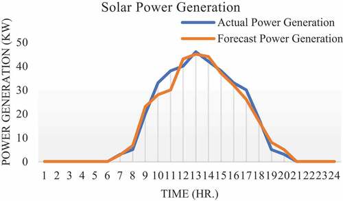
Figure 4. Wind power generation curve.

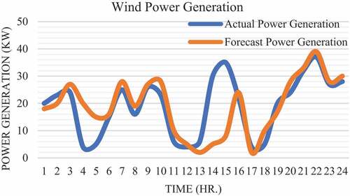
The error prediction for MSE, RMSE, and MAE are given in Table 1. The MSE is 6.122, RMSE is 2.474, and MAE is 1.495 for solar power generation and for wind power generation MSE is 78.25, RMSE is 3.034, and MAE is 5.41 calculated for a typical day.

Table 1. Error for solar PV and wind power generation.

Generation Source	MSE	RMSE	MAE
Solar PV Generation	6.122	2.474	1.495
Wind Power Generation	78.25	3.034	5.41

Energy consumption forecast model

This generated power is supplied to consumers and for this a price mechanism is developed, and forecast for the consumption at consumer end is shown in Figures 5, 6, and 7, respectively, for fixed, non-shiftable, and shiftable loads.

Figure 5. Energy consumption for fixed loads.

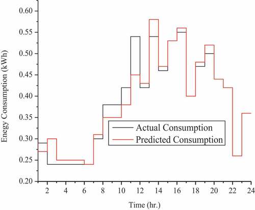
Figure 6. Energy consumption for non-shiftable loads.

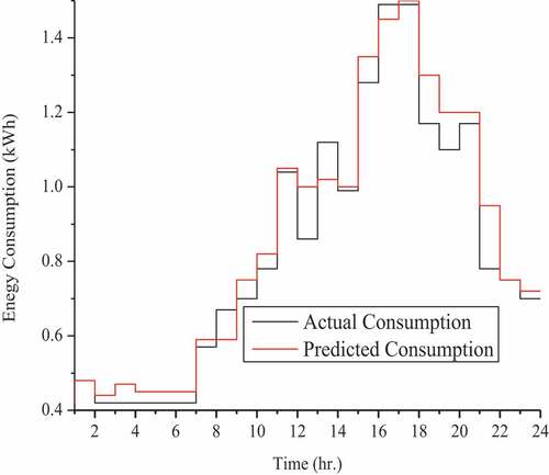
Figure 7. Energy consumption for shiftable loads.

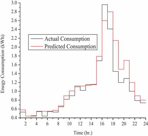
Actual and forecast energy usages in kWh for fixed loads are shown in Figure 5, and the MSE, RMSE, and MAE values are 0.0007, 0.027, and 0.0175, respectively. Figure 6 depicts a graph comparing uninterruptible (non-shiftable) loads energy consumption between actual and anticipated consumption, with MSE, RMSE, and MAE values of 0.0045, 0.067, and 0.049, respectively. The relationship between actual and anticipated energy usage for interruptible (shiftable) loads is shown in Figure 7, and the model generates sufficient results for consumption prediction at the consumer end, as indicated by MSE of 0.047, RMSE of 0.21, and MAE of 0.13. The compiled error report for energy prediction for different categories of appliances at consumer end is displayed in Table 2.

Table 2. Error for energy consumption prediction for types of loads.

Appliance type	MSE	RMSE	MAE
Fixed loads	0.0007	0.027	0.0175
Non-shiftable loads	0.0045	0.067	0.049
Shiftable loads	0.047	0.21	0.13

The results show that the proposed methods for predictions of solar and wind power generation and energy consumption forecast achieve better accuracy. The presented methodologies can be implemented for renewable energy predictions and loads predictions considering different categories. The presented results can be used further for doing demand-side management in coordination with renewable energy predictions for energy balancing. The presented results can be used for doing energy throughput using the appropriate energy storage capacity for maximizing the sustainable energy productions in coordination with demand-side management.

Conclusion

The energy management of the sustainable electrical energy network needs appropriate predictions from renewable energy sources as well as demand predictions. Machine learning tools (e.g. CNN) based on some pattern analyses are necessary for doing appropriate energy management considering renewable energy generation. The LSTM is a good tool for time-series forecasting using available sequential data and it is more appropriate for demand forecasting. In this work, CNN is used for predicting the solar and wind energy generation and forecasting of demand consumptions of some selected types/categories of loads via LSTM. The presented results have shown very good accuracy, and prediction errors are analyzed by MSE, RMSE, and MAE. The results are nearly accurate, with very little degree of error in prediction and the actual values. The MAE error for solar is 1.495 and that for wind energy generation is 5.41. It is necessary for doing energy management to have accurate demand predictions for selected categories of loads for managing the flexibility within the electrical energy network. In this work, LSTM method is used to predict the energy consumption and the MAE error for fixed load is 0.0175; for non-shiftable load, it is 0.049; and for shiftable load, it is 0.13. The results show that the proposed methods for predictions of solar and wind power generation and energy consumption forecast achieve better accuracy. The presented methodologies for renewable energy and demand predictions can be effectively used for demand-side management within electrical energy network and can also contribute to grid energy balancing through energy storage.

Nomenclature

PV	=	Photovoltaic
DNN	=	Deep neural network
CNN	=	Conventional neural network
RNN	=	Recurrent neural network
LSTM	=	Long short-term memory
RES	=	Renewable energy sources
MSE	=	Mean square error
RMSE	=	Root mean square error
MAE	=	Mean absolute error
Symbols	=
${\mathbf{X}}_{\mathbf{i}\left(\mathbf{t}\right)}$	=	Sequence of solar-wind power generated
${\mathbf{G}}_{\mathbf{input}}$	=	Historical solar and wind power generation data
${\mathbf{y}}_{\mathbf{i}}^1$	=	Output of the first convolutional layer
${\mathbf{W}}_{\mathbf{m}}^1$	=	Weight matrix for first convolutional layer
$\mathbf{m}$	=	Filter index value
${\mathbf{b}}_{\mathbf{i}}^1$	=	Bias in the convolution layer
${\mathbf{y}}_{\mathbf{i}}^2$	=	Output of the second convolutional layer
${\mathbf{y}}_{\mathbf{i}}^{\mathbf{n}}$	=	Output of the nth convolutional layer
${\mathbf{P}}_{{\mathbf{a}}_{\mathbf{s}}}$	=	Real power consumption of shiftable appliance
${\mathbf{t}}_{\mathbf{s},{\mathbf{a}}_{\mathbf{s}}}$	=	Starting time of shiftable appliances
${\mathbf{t}}_{\mathbf{d},{\mathbf{a}}_{\mathbf{s}}}$	=	End time of shiftable appliances
ϼ(t)	=	Proposed energy consumption price
${\mathbf{a}}_{\mathbf{sn}}$	=	Non-shiftable appliances
${\mathbf{P}}_{{\mathbf{a}}_{\mathbf{sn}}}$	=	Real-power consumed by non-shiftable appliances
${\mathbf{P}}_{\mathbf{l}}$	=	Total power losses at consumer end
${\mathbf{Q}}_{\mathbf{l}}$	=	Yotal reactive power losses at consumer end
${\mathbf{i}}_{\mathbf{g}}$	=	Input gate function
${\mathbf{f}}_{\mathbf{g}}$	=	Forget gate function
${\mathbf{o}}_{\mathbf{g}}$	=	Output gate function
${\mathbf{w}}_{{\mathbf{i}}_{\mathbf{g}}}$	=	Weight of input gate
${\mathbf{w}}_{{\mathbf{f}}_{\mathbf{g}}}$	=	Weight of output gate
${\mathbf{w}}_{{\mathbf{o}}_{\mathbf{g}}}$	=	Weight of forget gate
${\mathbf{x}}_{\mathbf{g}}$	=	Input for the existing gate
${\mathbf{h}}_{\mathbf{g}-1}$	=	Output of the previous gate
$\mathbf{b}$	=	Bias term
${\mathbf{Y}}_{\mathbf{act}}$	=	Actual consumption
${\mathbf{Y}}_{\mathbf{pre}}$	=	Anticipated consumption

Disclosure statement

No potential conflict of interest was reported by the authors.

Additional information

Notes on contributors

Akash Talwariya

Dr. Akash Talwariya received the B.Tech. in Electrical Engineering, M.Tech. in Power System from Rajasthan Technical University, Kota, Rajasthan, India in 2011 and 2015 respectively. Ph.D. degree in Electrical Engineering from JK Lakshmipat University, Jaipur, Rajasthan, India. He did post-graduation in Artificial Intelligence and Machine Learning from National Institute of Technology, Warragal, India. He joined L&T EduTech as Teaching Associate and current job profile is to create content for Electrical Engineering courses. His current research interest includes smart grids, game theory, machine learning, demand side management and future network architectures.

Pushpendra Singh

Dr. Pushpendra Singh is Associate Professor, Department of Electrical Engineering at JK Lakshmipat University, Jaipur. He did his Master of Technology and Doctorate from Malaviya National Institute of Technology (MNIT) Jaipur. With over Eighteen years of teaching, research, and administrative experience, he has held various administrative positions in the capacity of Principal, Head of Department. In his 18 years teaching, administrative and research duration he has published 85 research papers including high repute international journals, international conferences. He has 8 patent grants, 9 patents published, and one copyright granted in his account. Under his guidance two candidates have completed PhD degree. He is Senior member-IEEE, SM- IIIE and Fellow-IE(India). He is editorial member and advisory board member of quite a few international journals. His research area includes power system restructuring, power quality, integration of DERs, demand side management, power system stability, smart grid, distributed generators etc.

Jalpa H. Jobanputra

Dr. Jalpa H Jobanputra (Jalpa Thakkar) is working as an Associate Professor and Head of Department of Electrical Engineering at UPL University of Sustainable Technology in India. She has done Masters in Electrical Power System Engineering with Gold Medal from Gujarat Technological University and PhD in Electrical Power Transmission Management. She has more than a decade of Experience in Academics and Research in the Field of Electrical Engineering.

Mohan Lal Kolhe

Prof. Dr. Mohan Lal Kolhe is a full professor in smart grid and renewable energy at the Faculty of Engineering and Science of the University of Agder (Norway). He is a leading renewable energy technologist with three decades of academic experience at the international level and previously held academic positions at the world's prestigious universities, e.g., University College London (UK / Australia), University of Dundee (UK); University of Jyvaskyla (Finland); Hydrogen Research Institute, QC (Canada); etc. In addition, he was a member of the Government of South Australia’s first Renewable Energy Board (2009-2011) and worked on developing renewable energy policies. Due to his enormous academic contributions to sustainable energy systems, he has been offered the posts of Vice-Chancellor of Homi Bhabha State University Mumbai (Cluster University of Maharashtra Government, India), full professorship(s) / chair(s) in 'sustainable engineering technologies/systems' and 'smart grid' from the Teesside University (UK) and Norwegian University of Science and Technology (NTNU) respectively. He has successfully won competitive research funding from the prestigious research councils (e.g., Norwegian Research Council, EU, EPSRC, BBSRC, NRP, etc.) for his work on sustainable energy systems. His research works in energy systems have been recognized within the top 2% of scientists globally by Stanford University’s 2020, 2021, 2022 matrices. He is an internationally recognized pioneer in his field, who’s top 10 published works have an average of over 200 citations each.

References

- Agrawal, H., A. Talwariya, A. Gill, A. Singh, H. Alyami, W. Alosaimi, and A. Ortega-Mansilla. 2022. A fuzzy-genetic-based integration of renewable energy sources and E-Vehicles. Resources Policy 15 (9):3300. doi:10.3390/en15093300.
- Ahmad, S., A. Ahmad, M. Naeem, W. Ejaz, and H. S. Kim. 2018. A compendium of performance metrics, pricing schemes, optimization objectives, and solution methodologies of demand side management for the smart grid. Energies 11 (10):2801. doi:10.3390/en11102801.
- Baldi, S., Korkas, M. Lv, and E. B. Kosmatopoulos. 2018. Automating occupant-building interaction via smart zoning of thermostatic loads: A switched self-tuning approach. Applied Energy 231:1246–58. Dec. doi: 10.1016/j.apenergy.2018.09.188.
- Carley, S., E. Baldwin, L. M. MacLean, and J. N. Brass. 2017. Global expansion of renewable energy generation: An analysis of policy instruments. Environmental and Resource Economics 68 (2):397–440. doi:10.1007/s10640-016-0025-3.
- Gard-Murray, A. 2022. De-risking decarbonization: Accelerating fossil fuel retirement by shifting costs to future winners. Global Environmental Politics 22 (4):70–94. doi:10.1162/glep_a_00689.
- Ghaderi, A., B. M. Sanandaji, and F. Ghaderi. 2017. arXiv preprint arXiv:1707.08110, Deep forecast: Deep learning-based spatio-temporal forecasting. 1–6.
- Johannesen, N. J., M. L. Kolhe, and M. Goodwin, “Load demand analysis of nordic rural area with holiday resorts for network capacity planning”, In 4th International Conference on Smart and Sustainable Technologies (SpliTech), Croatia, 2019a, pp. 1–7. IEEE.
- Johannesen, N. J., M. L. Kolhe, and M. Goodwin. 2019b. Relative evaluation of regression tools for urban area electrical energy demand forecasting. Journal of Cleaner Production 218:555–64. doi:10.1016/j.jclepro.2019.01.108.
- Johannesen, N. J., M. L. Kolhe, M. Goodwin, “Comparing recurrent neural networks using principal component analysis for electrical load predictions,” 2021 6th International Conference on Smart and Sustainable Technologies (SpliTech), Bol and Split, Croatia, 1–6, 2021.
- Johannesen, N. J., M. L. Kolhe, and M. Goodwin. 2022. “Recurrent neural networks for electrical load forecasting to use in demand response”, chapter 3 of book ‘industrial demand response: Methods, best practices, case studies, and applications’, 41–58. UK: The Institution of Engineering and Technology.
- Khan, Z. A., T. Hussain, I. U. Haq, F. U. M. Ullah, and S. W. Baik. 2022. Towards efficient and effective renewable energy prediction via deep learning. Energy Reports 8:10230–43. doi:10.1016/j.egyr.2022.08.009.
- Liu, J., Q. Shi, R. Han, and J. Yang. 2021. A hybrid GA–PSO–CNN model for ultra-short-term wind power forecasting. Energies 14 (20):6500. doi:10.3390/en14206500.
- Li, Y., W. Xue, T. Wu, H. Wang, B. Zhou, S. Aziz, and Y. He. 2021. Intrusion detection of cyber physical energy system based on multivariate ensemble classification. Energy 218:119505. doi:10.1016/j.energy.2020.119505.
- Malakouti, S. M., A. R. Ghiasi, A. A. Ghavifekr, and P. Emami. 2022. Predicting wind power generation using machine learning and CNN-LSTM approaches. Wind Engineering 46 (6):0309524X221113013. doi:10.1177/0309524X221113013.
- Mathew, M. S., M. L. Kolhe, “Performance modelling of renewable energy systems using kNN algorithm for smart grid applications,” 2022 7th International Conference on Smart and Sustainable Technologies (SpliTech), Split/Bol, Croatia, 1–4, 2022.
- Nam, K., S. Hwangbo, and C. Yoo. 2020. A deep learning-based forecasting model for renewable energy scenarios to guide sustainable energy policy: A case study of Korea. Renewable and Sustainable Energy Reviews 122:109725. doi:10.1016/j.rser.2020.109725.
- Singh, P., A. Talwariya, and M. Kolhe. Aug 2019b. Demand response management in the presence of renewable energy sources using stackelberg game theory. In IOP Conference Series: Materials Science and Engineering. Vol. 605(1), 012004. IOP Publishing
- Talwariya, A., and P. Singh. Feb 2018. Demand side management: A survey of SPT & TOU. International Journal of Creative Research Thoughts 6(1):1675–78.
- Talwariya, A., P. Singh, M. D. Brinda, J. Jobanputra, & M. L. Kolhe, “Domestic energy consumption forecasting using machine learning”, In 2022 7th International Conference on Smart and Sustainable Technologies (SpliTech), Croatia. pp. 1–4. July 2022, IEEE.
- Talwariya, A., P. Singh, and M. Kolhe. 2019. A stepwise power tariff model with game theory based on monte-carlo simulation and its applications for household, agricultural, commercial and industrial consumers. International Journal of Electrical Power & Energy Systems vil. 111:14–24. Oct. doi: 10.1016/j.ijepes.2019.03.058.
- Talwariya, A., P. Singh, and M. L. Kolhe. 2021. Stackelberg game theory based energy management systems in the presence of renewable energy sources. IETE Journal of Research 67 (5):611–19. doi:10.1080/03772063.2020.1869109.
- Talwariya, A., P. Singh, and M. L. Kolhe. 2022. A stackelberg game theory based demand response algorithm for domestic consumers. Electric Power Components & Systems 50 (19–20):1186–99. doi:10.1080/15325008.2022.2150914.
- Talwariya, A., P. Singh, M. Kolhe, and J. H. Jobanputra. May 2020. Fuzzy logic controller and game theory based distributed energy resources allocation. AIMS Energy 8(3):474–92. doi: 10.3934/energy.2020.3.474.
- Talwariya, A., P. Singh, M. Kolhe and S. K. Sharma, “A game theory approach and tariff strategy for demand side management”, 3rd International Conference and Workshops on Recent Advances and Innovations in Engineering (ICRAIE), Jaipur, India. (pp. 1–5). IEEE, Nov. 2018.
- Wang, H., R. Cai, B. Zhou, S. Aziz, B. Qin, N. Voropai, E. Barakhtenko, and E. Barakhtenko. 2020. Solar irradiance forecasting based on direct explainable neural network. Energy Conversion and Management 226:113487. doi:10.1016/j.enconman.2020.113487.
- Wang, H., Z. Lei, X. Zhang, B. Zhou, and J. Peng. 2019. A review of deep learning for renewable energy forecasting. Energy Conversion and Management 198:111799. doi:10.1016/j.enconman.2019.111799.
- Zhang, R., G. Li, S. Bu, G. Kuang, W. He, Y. Zhu, and S. Aziz. 2022. A hybrid deep learning model with error correction for photovoltaic power forecasting. Frontiers in Energy Research 1103. doi:10.3389/fenrg.2022.948308.
- Zhang, C., H. Zhai, L. Cao, X. Li, F. Cheng, L. Peng, X. Wang, J. Meng, L. Yang, and X. Wang. 2022. Understanding the complexity of existing fossil fuel power plant decarbonization. Iscience 25 (8):104758. doi:10.1016/j.isci.2022.104758.