CarbonRoadMap: A multicriteria decision tool for multimodal transportation

Abstract

This article proposes a multicriteria approach and a decision support system to support multimodal transportation planning decisions by considering transportation delay, costs, and carbon emissions. The methodology is implemented into CarbonRoadMap, a web-based application that allows a decision maker to browse through the set of Pareto-optimal paths, display them on a map to support the selection of the desired optimum solution by weighting the three criteria. This decision support tool shows the benefits of using a multicriteria optimization methodology to obtain a set of paths, as the resulting solutions are very different from one another. A case study is provided for forest product distribution in North America.

Keywords:

• Carbon emissions
• decision support system
• multimodal transportation
• multiobjective optimization

1. Introduction

In the past decade, carbon concentration in the atmosphere has increased significantly (NOAA, 2016). According to the Intergovernmental Panel on Climate Change (IPCC), this increase is mainly anthropogenic and causes climate change (IPCC, 2014). Due to fossil fuel consumption, the logistics and transportation sector accounts for 5.5% of the global carbon emissions (World Economic Forum, 2009). Road transport alone accounted for close to 80% of the 1.8 Gt CO₂ equivalent issued by the entire transport sector (EIA, 2015). Since the adoption of the Kyoto protocol, a collective awareness of the consequences of climate change has arisen and intensive efforts are being made to reduce anthropogenic carbon emissions. More customers are now interested in the ecological and carbon footprints associated with the products they use. This creates pressure for companies to lower their carbon footprint while keeping costs under control.

Yet, most logistics decisions, such as freight transportation of goods, are typically based on economic criteria such as costs, often paired with delivery time considerations (SteadieSeifi, Dellaert, Nuijten, Van Woensel, & Raoufi, 2014), with little or no consideration for carbon emissions in the decision process. Since the usual means of transport are frequently energy intensive and great emitters of greenhouse gases (Winebrake, Green, Comer, Corbett, & Froman, 2012), it is timely to develop new tools to improve decision making that includes costs, time as well as carbon emissions.

The efficiency (fuel consumption per ton.kilometer) varies according to the modes of transport. Carbon efficiency (carbon emissions per t.km) is also variable. Each transportation mode has advantages. So, multimodal transportation appears to be one of the key strategies to reduce the carbon footprint of products, as it allows companies to reduce distribution costs while also reducing carbon emissions (World Economic Forum, 2009). However, planning and execution of multimodal transportation are more complex and requires a higher degree of coordination (Caris, Macharis, & Janssens, 2013). The decision support system (DSS) that we developed and is presented in this article can support companies to find good tradeoffs between reduction of the carbon footprint associated with transportation activities, improving delivery times and meeting cost standards.

This article presents a new methodology to support operational transportation planning decisions based on multicriteria optimization. This methodology is embedded into CarbonRoadMap, a web-based DSS which is presented in Section 3. The article also includes a case study (Section 4) associated with a forest products company in Canada, demonstrating how CarbonRoadMap can be used in practice. Section 5 presents the solutions obtained with the DSS and the conclusions are presented in Section 6.

2. Background

Many industries can benefit from reduction of their carbon footprint (Endrikat, Guenther, & Hoppe, 2014; Lash & Wellington, 2007; Plambeck, 2012). Many studies have shown replacing building materials with wooden alternatives can lead to carbon emission reduction, since wooden building materials are less energy intensive, and consequently, produce fewer carbon emissions than building materials as steel and concrete (Lucon et al., 2014). However, this advantage may be counterbalanced by truck transportation due to large distances between the production construction sites, particularly in North America. A Life-Cycle Assessment (LCA) performed on glued-laminated wood timber (glulam) from Quebec's boreal forest applied in a building has shown that extraction and production emit 110 kgCO₂eq. per cubic meter of glulam (Laurent et al., 2013). The Life-Cycle Inventory shows that glulam beams travel an average of 1,000 km to reach the construction site. Total carbon emissions from road transport over such distances with an assumed rate of no-load returns are 150 kgCO₂eq. per cubic meter of glulam, 140% of the carbon emissions of the previous stages of the life cycle. It seems necessary to provide solutions to reduce the impacts of this distribution step.

Wood products transportation is often carried out by truck, even though the use of alternative transportation means, such as train and ship, may reduce the delivery carbon footprint (Winebrake et al., 2012). To test this hypothesis, we developed an algorithm that generates maps showing carbon emissions from different modes of transport (truck, train, and boat). The lines on the map, representing possible paths, change color depending on carbon emissions. This makes it possible to compare the distance reachable only by truck (Figure 1) and by multimodal transport (Figure 2) with carbon emissions below defined levels. This is what we call the boundaries of carbon efficiency. For this example, the origin is located in Chibougamau, Quebec, located at coordinates (49.929704, -74.376411), where glulam beams are produced from boreal forest trees.

Figure 1. Truck-only carbon efficient boundary. The blue line represents carbon emissions under 50 kgCO₂eq. The red line represents carbon emission over 150 kgCO₂eq.

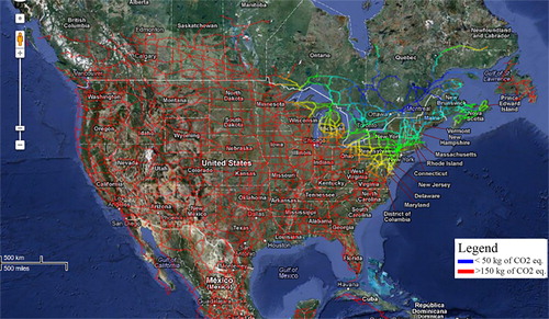
Figure 2. Intermodal carbon efficient boundary. The blue line represents carbon emissions under 50 kgCO₂eq. The red line represents carbon emission over 150 kgCO₂eq.

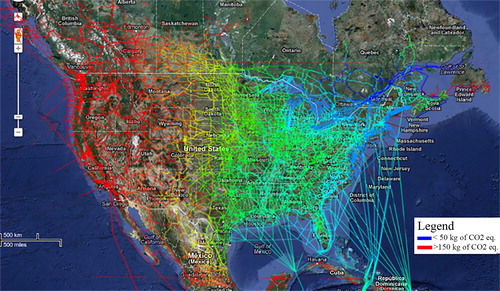
A significant portion of North America can then be covered below the maximum carbon emission level. In this way, six Canadian provinces and 39 United States can now be reached within the 150 kgCO₂eq. efficiency limit.

From this analysis, it is clear that there is potential for reduction of the carbon footprint from transportation by multimodal transportation instead of monomodal transportation. It has a great potential to support transportation managers to find multimodal routes that meet their preferences and needs. Although, interesting, roads that only consider minimizing carbon emissions are unlikely to be used in practice because they do not meet the needs of manufacturers who have to also take into account costs and delivery times into their decisions.

Intermodal transportation has been the subject of research in the last few years; comprehensive reviews are provided in SteadieSeifi et al. (2014) and Caris et al. (2013). Despite abundant literature in the field, multiobjective models accounting for both cost and delivery time have only appeared recently; Yang, Low, and Tang (2011) propose a goal programing model minimizing transportation costs and travel time. The minimization of carbon emissions associated with intermodal transportation is scarcely reported. Bauer, Bektaş, and Crainic (2010) propose a model to incorporate greenhouse gas emissions into service network design problems. Rudi, Fröhling, Zimmer, and Schultmann (2014) propose a multicommodity network flow model incorporating costs, carbon emissions and transportation delays; to the best of our knowledge, it is the only model incorporating these three criteria in tactical multimodal transportation planning problems. However, the study of Rudi et al. (2014) describes a tactical planning context, where a set of carriers must be selected for each transportation arc. As a result, a great part of the mathematical model proposed is dedicated to accurately modeling contracts and restrictions associated with the choice of carriers. In addition, the model allows for specific quantities of different products that must be shipped from various origins to various destinations. The planning context of the DSS model we present is more operational and plans for the shipment of make-to-order products (glulam beams) on an individual basis. Long-term contracts with carriers are usual in the forest product industry; therefore the choice of carriers in each region does not need to be included in the planning model. Our method also differs: while the DSS of Rudi et al. (2014) requires the user to set weights associated with each criterion, our approach allows for the generation of all nondominated paths (paths without any prior weighting). Moreover, we use a much larger size of the network with millions of nodes and edges compared to 57 nodes and 90 edges in the DSS of Rudi et al. (2014). With this large network, CarbonRoadMap is designed to use road databases directly in the modeling.

3. Methodology proposed multimodal DSS system

We developed a DSS to determine which transportation mode, or which combination of transportation modes, and which route should be used to deliver a specific product, while optimizing delivery time, costs, and carbon emissions. For any origin and any number of destinations, the approach consists of building a network representation of all potential paths to the destination(s). Considering the duration, costs, and carbon emissions associated with each feasible route, the tool effectively finds all nondominated routes and presents the user with the best route according to their preferences.

3.1. Data requirements and network representation

To evaluate the best routes available, an integrated network representation was developed. For this we needed high-quality GIS data of North America that we obtained using the National Atlas Database provided by the US Department of Transportation’s Bureau of Transportation Statistics (USDoTBTS).

Formally, the integrated multimode transportation network is represented as a directed multigraph, with a set of nodes and a set of arcs. The arcs represent route segments that allow a product to move from one location to another. It can represent a segment of a road, of a railroad or the route of a ship between two ports. In the multigraph, the nodes merely represent connecting points between various transportation arcs. Each arc has a set of specific attributes, such as a length (in kilometers), average transportation speed, availability, transportation modes used, whether the arc is used to connect different transportation modes or not, and whether the arc crosses an international border or not. Attributes represent properties of the transportation network and are independent of the characteristics of the freight being transported or the user of the DSS. These attributes are used to calculate context-specific factors that will be used in the optimization. Section 3.2 describes how the values of each criterion (carbon emission, delivery time and costs) are derived using a function based on the arc attributes.

The use of a multigraph is also very important to model real-world transportation costs structures. As shown in Martel (2005), the relationship between distance and transportation costs in North America is usually nonlinear, showing important economies of scale; this is especially true for the main freight corridors linking major urban and industrial areas.

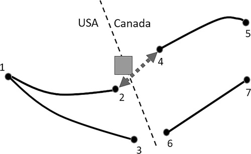
Typically, the road networks from different countries are not properly connected, even when the road databases come from the same source. In practice, many roads end at national or state borders without actually crossing the border. Connecting segments across borders which are closer than a predetermined threshold distance would create unrealistic networks and would in particular underestimate the distance required to cross borders. Instead, the following procedure has been implemented to interconnect the segments in the database. For each checkpoint, the closest road segment on each side of the border was determined. Then, an additional arc was inserted in the network connecting these two road segments. The additional costs and delays associated with customs border crossing are also added to this arc. Figures 3 and 4 show an example of such a network where different unconnected road segments are close to a border. The square represents a customs checkpoint between Canada and the United States. The road segment closest to the checkpoint on the United States side ends in Node 2; the closest segment on the Canadian side ends in Node 4. Thus, an additional arc is inserted that connects Nodes 2 and 4 (Figure 4). Although, Nodes 3 and 6 are closer to each other than Nodes 2 and 4, they remain unconnected.

Figure 3. Network before connection.

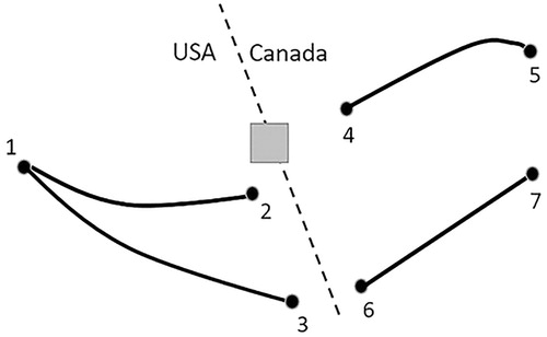
Figure 4. Network after connection. Arc 2-4 is inserted.

The same procedure was used to connect the rail transportation networks of different railroad companies, as well as intermodal transportation terminals.

3.2. Calculation arc factors

Attributes that are composed in our database are: arc length (in km) of different types (road, railway, maritime way, harbor [maritime way to road transition], train station [railway to road transition], dock [railway to maritime way transition], and customs [road-to-road transition]). Each of those types needs to be converted in factors related to our criteria: carbon emission, delivery time and cost. We used a linear model to convert arc length in carbon emission (Fe), time (Ft), and cost (Fc) factors. Each of the three factors is calculated by multiplying the variable parameters (ve, vt, vc) with the distance d of the arc (in km) and the fixed parameters (fe, ft, fc) are added up. Transition arcs have a distance of 0 km. (1) $$\mathrm{F}\mathrm{e}=\mathrm{f}\mathrm{e}+\mathrm{v}\mathrm{e}\times d$$(1) (2) $$\mathrm{F}\mathrm{t}=\mathrm{f}\mathrm{t}+\mathrm{v}\mathrm{t}\times d$$(2) (3) $$\mathrm{F}\mathrm{c}=\mathrm{f}\mathrm{t}+\mathrm{v}\mathrm{t}\times d$$(3)

The next table gives the fixed (fe, ft, fc) and the variable parameters (ve, vt, vc) per type of arc. Carbon parameters are based on the ecoinvent database (ecoinvent Center, St-Gallen, Switzerland). Other parameters are arbitrarily set to realistic values. The parameters presented in the Table 1 can be adjusted to fit the unique situation of a company.

Table 1. Factors for all criteria by cubic meter of glulam.

		Carbon (kgCO2eq.)	Cost (CAD)	Time (h)
Variable parameters	Road	0.08241	0.0205	0.01
	Railway	0.00581	0.0105	0.25
	Maritime way	0.02566	0.00235	0.05
Fixed parameters	Harbor	0	5	5
	Train station	0	3	3
	Dock	0	5	5
	Customs	0	1	0.2

3.2.1. Carbon emissions

In a recent survey Demir et al. (2014) listed and analyzed 25 different models to estimate carbon emissions associated to freight transportation. The intensity of carbon emissions from transportation activities varies due to many factors: loads, vehicle condition, and driving habits such as speed and acceleration (Ahn, Rakha, Trani, & Van Aerde, 2002). Ross (1997) uses analytical expressions to estimate carbon emissions based on energy consumption required to transport a given load; this approach is also used for rail transportation in Bauer et al. (2010). The macroscopic approaches, which rely on average speed over long driving distances, are those which are more suited to be implemented in the proposed methodology. We used an LCA-based approach to estimate emissions in line with the approach used by Quariguasi Frota Neto, Bloemhof-Ruwaard, van Nunen, and van Heck (2008). Indirect emissions are included in the calculation. Factors presented in Table 1 are from the ecoinvent database (version 2.2) (Hedemann & König, 2007) adapted to the North American context. Carbon emissions were calculated in SimaPro v7 (PRé Consultants, Amersfoort, The Netherlands) by the IPCC 2007 impact method using a global warming potential within 100 years (Solomon et al., 2007). Carbon emissions of the transshipment activities are neglected since they are difficult to calculate and very small compared to transport-related emissions (Rüdiger, Schön, & Dobers, 2016).

3.2.2. Costs estimations

Kay and Warsing (2009) proposed a model to estimate shipping rates for small to medium-sized loads (less-than-truckload rates) using only publicly available data. While simple linear functions can be used on short distance arcs, such as city streets, nonlinear models might be necessary to accurately estimate the cost of long-distance arcs between main transportation hubs (Kay & Warsing, 2009). Although, the model considers only full loads, the transport cost structures follow the usual components of fixed and variable costs (Martel, 2005). Fixed cost components are based on the intermodal terminals (harbor, train station, dock, and customs), while the variable cost is based on the distance.

3.2.3. Delivery times

Delivery time functions are usually straightforward, depending mostly on the maximum driving speed allowed on the transportation arc as well as mean loading/unloading times. Other relevant attributes might differ between transportation modes; railroads, and ships may be subject to schedules, while road transportation is subject to a maximum number of driving hours per day. Road congestion is not taken into account in the model, but other aspects like intermodal transshipment or international border crossings are included. Time-dependent travel times can be included, although, with a significant additional computational load.

3.3. Optimization algorithm

Once the transportation network has been defined and interconnected and factors have been obtained for each transportation arc, potential routes $V$ from origin to destination can be evaluated. As the goal of CarbonRoadMap is to support decision makers rather than to automate decision making, we would like to obtain the set of dominant routes through a dominance test. By applying the dominance test when finding the shortest path in the graph, the set of all dominant routes is obtained. The dominance test can be expressed in terms of routes as follows: a route $V$ is dominated by a group $G$ of routes $P_i$ if there is no weight vector$\mathrm{ }W$which allows the scalar product between $V$ and $W$ to be less than each individual scalar product between $P_i$ and $W$; this rule is outlined in (4): (4) $$V\mathrm{ }\text{is} \text{dominated} \text{by} G\mathrm{ }\text{if} \left[\left(V\cdot W\right)>\left(P_i\cdot W\right)\right]\mathrm{ }\forall P_i\in G$$(4)

Formally, this problem can be modeled as a single source multiobjective shortest path problem; a mathematical formulation is provided in Raith and Ehrgott (2009). Although, this problem is intractable in general, previous research has shown that for transportation network applications the set of nondominated solutions is very small (Müller-Hannemann & Weihe, 2006). The three factors used as objectives in our model are:

• Emissions measured in CO₂ equivalents;

• Transportation delay, measured in hours;

• Total transportation costs, measured in Canadian dollars (CAD).

Solution methods for the multiobjective shortest path problem can be found in Raith and Ehrgott (2009) and Machuca, Mandow, Pérez de la Cruz, and Ruiz-Sepulveda (2012). Although, some solutions can be obtained by transforming the multiobjective shortest path problem into a single-objective shortest path using a weighted sum of the objectives, this approach only allows finding a subset of the optimal solutions (i.e., the set of supported nondominated paths). As we are interested in finding both supported and nonsupported nondominated shortest paths, a label-setting algorithm (Guerriero & Musmanno, 2001) was chosen instead.

The proposed algorithm is fast enough to remain tractable for networks of sizes up to more than a million arcs. However, building extended networks covering whole continents, such as North America or Europe, will result in exceedingly large multigraphs with tens of millions of arcs. To be used in such cases, the network should be pruned by removing arcs from lower-priority road classes to limit the size of the network.

3.4. Filtering solutions presented to the user

Although, the number of nondominated paths remains tractable, it can be too large for a user to go through all of it and select a single solution. As such, we proposed a method that helps the user in selecting a small set of solutions. Let S be the set of nondominated solutions found by the optimization algorithm. Instead of going through each solution one at a time, the user can select a weight $w_{}^f$ for each factor f, so that the sum of all weights equals one. Let $v_f^{\text{min}}$ and $v_f^{\text{max}}$ be the minimum and maximum value for factor f among all solutions in S, $W^f$ the user-set weight associated to factor f and $v_f^{\mathrm{*}}\mathrm{ }$the value for factor f associated to a given solution s. When the user sets weights, the solution that minimizes Equation (5)(5) $$s\in S\mathrm{ }\left\{\arg {\text{min}}_s:{\sum }_{i=0}^n{W}^f\left(\frac{v_f^{\mathrm{*}}-v_f^{\text{min}}}{v_f^{\text{max}}-v_f^{\text{min}}}\right)\right\}$$(5) is displayed to the user. (5) $$s\in S\mathrm{ }\left\{\arg {\text{min}}_s:{\sum }_{i=0}^n{W}^f\left(\frac{v_f^{\mathrm{*}}-v_f^{\text{min}}}{v_f^{\text{max}}-v_f^{\text{min}}}\right)\right\}$$(5)

For each factor, the solution $v_f^{\text{min}}\mathrm{ }$is of particular interest: it is the optimum path of the shortest path problem considering this factor only.

Identifying the optimal path involves applying the weights associated with the criteria (carbon, costs, time) to each nondominated vector and finding the nondominated vector associated with the path with the least impact on our weighted criteria.

3.5. CarbonRoadMap interface

To make the methodology suitable for use by a vast number of decision makers, it has been embedded into CarbonRoadMap, a web-based DSS. The interface of CarbonRoadMap was developed as a web-based application that is easily accessible through a web browser. The interface is developed mainly in C#, JavaScript and HTML in a .NET and Windows environment. The interface mainly consists of a map generated through Open Layers which uses OpenStreetMap maps. Three vertical scroll bars allow the user to define the relative weights of the three criteria [carbon (c), costs (m), and delay (d)]. Additionally, a fourth scroll bar allows the user to explore the set of optimal solutions, composing the Pareto front.

To make the system more versatile, two decision support modes are integrated. The single mode allows the user to obtain the optimal path for a single origin to a specific destination. The one-to-many mode allows the user to obtain the set of optimal paths leading to multiple destinations from a single origin. Such a set can be displayed on a map tile. This mode is used to precompute all destinations from an origin node to make faster representations of the optimized path for a given destination. The optimization algorithm was implemented as a C++ library that is called by the DSS when necessary.

4. Case study description

To perform a case study, the multimodal transportation network of North America was assembled and imported into the decision support tool. The road, rail and sea network data of the National Atlas Database 2011 were downloaded from the website of the United States of America’s Bureau of Transportation Statistics (BTS). The purpose of the case study is to demonstrate the applicability of the approach rather than to precisely reflect the operating context of a given company. As such, the functions chosen to obtain the factors are relatively simple to provide reasonable estimates.

Carbon emission factors for each transportation arc were obtained using data from the ecoinvent database modified to adapt the data to the energy mix typically used in North America. Thus, it is estimated that freight transportation emits on average 0.15 kgCO₂eq. per tkm, which corresponds to typical truck usage and fuel mix for wood transportation in North America (Laurent et al., 2013). It is assumed that vehicles—trucks, trains, or ships—are fully loaded and returns are not considered. This assumption was retained because transport operations are delegated to a dedicated service provider, which optimizes these charges and minimizes empty returns by loading other products. Costs and delivery times for road transportation, including customs border crossing, are estimated based on the average of several studies performed by the authors and their respective research teams at the FORAC Research Consortium. An estimate of costs and delivery times associated with rail transport was provided by the Canadian National (CN) company, which owns and operates the largest rail network in Canada. Estimates for the cost per tkm and traveling time by rail to various destinations in North America were also provided by the CN company.

For the case study, a cubic meter of glulam was chosen as functional unit of a shipment to be transported. Therefore, truck transport of a cubic meter of glulam emits 0.08 kgCO₂eq. per km. Similarly, emission factors for rail and ship transportation are respectively 0.025 and 0.0058 kgCO₂eq. per cubic meter of glulam km. Table 1 shows the factors used in the optimization to estimate the various criteria depending on the distance traveled.

The transshipments between transportation nodes, customs, and border crossings as well as usage of toll roads or ferries also have an impact on both costs and delivery time. Estimates from the CN company were used to assess these factors (Table 1) (CN sale service, personal communication, April 2012). The values-for-costs in Table 1 are given per cubic meter, while the values for delay are independent of the quantity transported. We assumed the factors of inverse transshipment to have the same value. Likewise, the above factors are determined for the transport as fully loaded.

5. Results and discussion

5.1. Case study results

To explore the results obtained by using CarbonRoadMap, we consider a delivery for a beam of glulam originating from the city of Chibougamau, located in Quebec (Canada), to a destination located in Sioux Falls, South Dakota, in the United States of America. This location was chosen due to its accessibility by road transportation (being close to Interstate-90), rail, as well as water (being close to the Missouri River). As such, it allows for many combinations between various transportation modes. More than one million nondominated paths exist between the origin and destination; only 72 are selected to be presented to the user after the filtering step described in Section 3.4. Only the optimal solutions for the three criteria and the values associated with each of the criteria are given in Table 2. To distinguish them, the minimum and maximum values obtained for each criterion when examining all nondominated solutions are provided in bold. The cost optimization solution seems to be a good compromise for this specific case study, since the result of the minimization of the costs gives a carbon value and a delivery time relatively close to the minimum possible values for the two criteria.

Table 2. Optimal solutions of the case study.

	$v_{}^{\text{carbon} \text{emissions}}$ (kgCO2eq. /m^3)	$v_{}^{\text{cost}}$ (CAD/m^3)	$v_{}^{\text{delivery} \text{time}}$ (h)	Total length of the optimal path (km)
Minimal delivery time	233,17	58,01	28,3	2829,59
Minimal carbon emissions	49,09	312,27	1242,7	4652,19
Minimal costs	69,54	19,14	138,47	2577,29

To show what CarbonRoadMap looks like, Figsures 5–7 show serigraphs of the graphical interphase representing the minimization solutions of the three criteria. The route minimizing carbon emissions in Figure 4, makes extensive use of waterways, from the St. Lawrence River to the Great Lakes and then to the Illinois and Missouri Rivers. It is not very attractive to transportation managers, as the costs are 16 times higher than the minimal costs route and the duration is more than 51 days, 43 times longer than the fastest path. The route minimizing transportation delay in Figure 5, corresponds to a direct delivery by truck, which can be done in 28 h and results in emissions of 233 kgCO₂eq. This option is currently the most common choice in the industry to transport glulam beams. Figure 7 provides the minimal costs solution; this route uses the railway for the most part. It takes 4.9 times more time but achieves a significant 66% in cost reduction as well as a 29.4% decrease in CO₂ emissions compared to carbon minimization, Figure 6.

Figure 5. CarbonRoadMap screen shot presenting the paths which minimize delay. For the delay minimization solution, the path is red because the only mode of transport used is the truck.

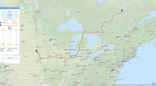
Figure 6. CarbonRoadMap screen shot presenting the paths which minimize carbon emissions. To minimize the carbon emission, train (green line) is used from Chibougamau, QC (origin) to reach the St. Lawrence River to be shipped by boat (blue line), and across the Great Lakes reaches the Mississippi and Missouri rivers, and finish the last mile by truck (red line) to Sioux Falls, SD (destination).

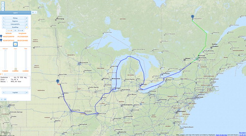
Figure 7. CarbonRoadMap screen shot presenting the paths that minimize costs. The train (green line) is the mode of transportation that minimizes the costs. Only the last kilometers are by truck, to reach the construction site.

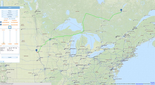
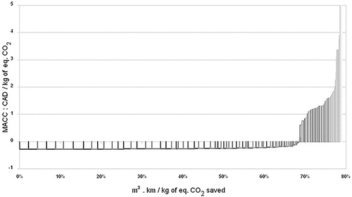
Figure 8. Marginal abatement cost curve showing results for the 60 largest cities in North America.

To be able to distinguish the use of the different modes of transport, each mode of transport is represented by a colored line in CarbonRoadMap. The red line is for the truck, the green is for the train, and the blue for the boat.

5.2. Abatement of carbon emissions

The examples provided in the previous sections are useful to outline what information can be derived from CarbonRoadMap for a single shipment. These conclusions are, however, too specific to help a company in making more general (tactical) decisions regarding their transportation mode selection policy. CarbonRoadMap’s one-to-many modes can be used for this purpose. We generated and analyzed the paths from Chibougamau, QC, to the 65 largest cities in North America regarding population. Expanding the number of destinations permits generating an interesting Marginal Abatement Cost Curve (MACC). A MACC is an effective way to show the extra (or “marginal”) cost of a solution to reduce (or to “abate”) carbon emissions, expressed in percentages, relative to a baseline (Kesicki & Strachan, 2011). In this context, the delay minimization path provides a sensible baseline because trucks are the only transportation mode currently used by Quebec glulam manufacturers.

The leftmost cube under the abscissa axis on the MACC represents the path leading to the largest improvements in costs and carbon emissions compared to the baseline (truck transportation); this path allows savings of up to 0.28$per kgCO₂eq emitted. Another interesting element is the point where the abatement curve crosses the abscissa, which represents the limit at which it is still possible to reduce both carbon emissions and transportation costs. This shows it is possibly profitable to decrease emissions by 70% compared to the truck-only solutions.

6. Conclusion

Transportation decisions are critical for a company’s supply chain performance but also to achieve significant carbon emission reductions. This article has proposed a methodology to build a multimodel transportation network and obtain the set of Pareto-optimal paths to reach either one or many destinations with a given point of origin and a set of optimization criteria (cost, carbon, and time). The algorithm used for this purpose allows generating all such paths through a single pass. This methodology has been implemented into CarbonRoadMap, a web-based decision support that allows a decision maker to browse through the set of Pareto-optimal paths and display them on a map.

A case study is presented for transporting glulam beams from northern Quebec with three optimization criteria: carbon emissions, costs, and transportation time. This case study shows the benefits of using a multicriteria methodology to obtain a set of paths, as the resulting solutions are very different from one another. This allows a manufacturer to select a route meeting the specific needs of each customer. On a higher level of decision making, we have shown that the DSS can also help in obtaining a broader picture of potential carbon emissions reduction of a portfolio of transport options and their impacts on costs and delays. When used in the context of producing building materials, it allows a company to control and manage the net carbon emissions associated with its products, which can be important in this industry. However, minimizing the transportation carbon footprint affects both costs and delivery time. To provide a full-personalized service, the wood manufacturer has to provide the customer with information on the three criteria to decide which type of delivery optimally serves the need of the customer.

The current model, designed for tactical planning, shows great potential for optimizing multicriteria transport, specifically the integration of carbon emission criteria. Some improvements are still possible, such as taking into account realistic data for carbon emissions resulting from transshipment activities. From an operational point of view, it would be relevant to add road traffic information to obtain a more realistic result regarding the delivery time. For strategic decision support, it could be interesting to suggest warehouse openings between production sites and customers, which could potentially reduce transportation costs and carbon emissions.

References

- Ahn, K., Rakha, H., Trani, A., & Van Aerde, M. (2002). Estimating vehicle fuel consumption and emissions based on instantaneous speed and acceleration levels. Journal of Transportation Engineering, 128(2), 182–190. doi:10.1061/(ASCE)0733-947X(2002)128:2(182)
- Bauer, J., Bektaş, T., & Crainic, T. G. (2010). Minimizing greenhouse gas emissions in intermodal freight transport: an application to rail service design. Journal of the Operational Research Society., 61(3), 530–542.
- Caris, A., Macharis, C., & Janssens, G. K. (2013). Decision support in intermodal transport: A new research agenda. Computers in Industry, 64(2), 105–112. doi:10.1016/j.compind.2012.12.001
- Demir, E., Bektas, T., Laporte, G. (2014). A review of recent research on green road freight transportation. European Journal of Operational Research, 237(3), 775–793. doi:10.1016/j.ejor.2013.12.033.
- EIA. (2015). Annual Energy Outlook 2015. U.S. Energy Information Administration. Washinton D.C., USA. https://www.eia.gov/outlooks/aeo/pdf/0383(2015).pdf
- Endrikat, J., Guenther, E., & Hoppe, H. (2014). Making sense of conflicting empirical findings: A meta-analytic review of the relationship between corporate environmental and financial performance. European Management Journal, 32(5), 735–751. doi:10.1016/j.emj.2013.12.004
- Guerriero, F., & Musmanno, R. (2001). Label correcting methods to solve multicriteria shortest path problems. Journal of Optimization Theory and Applications, 111(3), 589–613. doi:10.1023/A:1012602011914
- Hedemann, J., & König, U. (2007). Technical documentation of the ecoinvent database. Dübendorf, CH: Swiss Centre for Life Cycle Inventories.
- IPCC, I.P. on C.C. (2014). (Ed.), Climate change 2014: mitigation of climate change: Working Group III contribution to the Fifth Assessment Report of the Intergovernmental Panel on Climate Change. New York, NY: Cambridge University Press.
- Kay, M. G., & Warsing, D. P. (2009). Estimating LTL rates using publicly available empirical data. International Journal of Logistics Research and Applications, 12(3), 165–193. doi:10.1080/13675560802392415
- Kesicki, F., & Strachan, N. (2011). Marginal abatement cost (MAC) curves: confronting theory and practice. Environmental Science & Policy, 14(8), 1195–1204. doi:10.1016/j.envsci.2011.08.004
- Lash, J., & Wellington, F., (2007). Competitive advantage on a warming planet. Harvard Business Review, 85(3), 94–102, 143.
- Laurent, A.-B., Gaboury, S., Wells, J.-R., Bonfils, S., Boucher, J.-F., Sylvie, B., … Villeneuve, C. (2013). Cradle-to-gate life-cycle assessment of a glued-laminated wood product from Quebec’s Boreal forest. Forest Products Journal, 63(5–6), 190–198. doi:10.13073/FPJ-D-13-00048
- Lucon, O., Ürge-Vorsatz, D., Zain Ahmed, A., Akbari, H., Bertoldi, P., Cabeza, L. F., … Vilariño, M. V. (2014). Buildings. In O. Edenhofer, R. Pichs-Madruga, Y. Sokona, E. Farahani, S. Kadner, K. Seyboth, … J. C. Minx (Eds.), Climate Change 2014: Mitigation of Climate Change. Contribution of Working Group III to the Fifth Assessment Report of the Intergovernmental Panel on Climate Change, Chapter 9. In O R Edenhofer (Eds.), Cambridge University Press, Cambridge.
- Machuca, E., Mandow, L., Pérez de la Cruz, J. L., & Ruiz-Sepulveda, A. (2012). A comparison of heuristic best-first algorithms for bicriterion shortest path problems. European Journal of Operational Research., 217(1), 44–53. doi:10.1016/j.ejor.2011.08.030
- Martel, A. (2005). The design of production-distribution networks: a mathematical programming approach. In J. Geunes, P. M. Pardalos (Eds.), Supply chain optimization, applied optimization., 98, 265–305, Springer, U.S. doi:10.1007/0-387-26281-4_9
- Müller-Hannemann, M., & Weihe, K. (2006). On the cardinality of the Pareto set in bicriteria shortest path problems. Annals of Operations Research, 147(1), 269–286. doi:10.1007/s10479-006-0072-1
- NOAA. (2016). ESRL Global Monitoring Division - Global Greenhouse Gas Reference Network. Retrieved from http://www.esrl.noaa.gov/gmd/ccgg/trends/
- Open Layers. Retrieved from http://openlayers.org/
- OpenStreetMap maps. Retrieved from http://www.openstreetmap.org/
- Plambeck, E. L. (2012). Reducing greenhouse gas emissions through operations and supply chain management. Energy Economics, Green Perspectives, 34, S64–S74. doi:10.1016/j.eneco.2012.08.031
- Quariguasi Frota Neto, J., Bloemhof-Ruwaard, J. M., van Nunen, J. A. E. E., & van Heck, E. (2008). Designing and evaluating sustainable logistics networks. International Journal of Production Economics, 111(2), 195–208. doi:10.1016/j.ijpe.2006.10.014
- Raith, A., & Ehrgott, M. (2009). A comparison of solution strategies for biobjective shortest path problems. Computers & Operations Research, 36(4), 1299–1331. doi:10.1016/j.cor.2008.02.002
- Ross, M. (1997). Fuel efficiency and the physics of automobiles. Contemporary Physics, 38(6), 381–394. doi:10.1080/001075197182199
- Rudi, A., Fröhling, M., Zimmer, K., & Schultmann, F. (2014). Freight transportation planning considering carbon emissions and in-transit holding costs: a capacitated multi-commodity network flow model. EURO Journal on Transportation and Logistics, 1, 38. doi:10.1007/s13676-014-0062-4
- Rüdiger, D., Schön, A., & Dobers, K. (2016). Managing greenhouse gas emissions from warehousing and transshipment with environmental performance indicators. Transportation Research Procedia Arena TRA2016, 14, 886–895. doi:10.1016/j.trpro.2016.05.083
- Solomon, S., Qin, D., Manning, M., Chen, Z., Marquis, M., Averyt, K. B., … Miller, H. L. (2007). Climate Change 2007: The Physical Science Basis. Contribution of Working Group I to the Fourth Assessment Report of the Intergovernmental Panel on Cli mate Change. IPCC. Cambridge, UK/New York, NY: Cambridge University Press.
- SteadieSeifi, M., Dellaert, N. P., Nuijten, W., Van Woensel, T., & Raoufi, R. (2014). Multimodal freight transportation planning: A literature review. European Journal of Operational Research., 233(1), 1–15. doi:10.1016/j.ejor.2013.06.055
- Winebrake, J. J., Green, E. H., Comer, B., Corbett, J. J., & Froman, S. (2012). Estimating the direct rebound effect for on-road freight transportation. Energy Policy, Special Section: Frontiers of Sustainability, 48, 252–259. doi:10.1016/j.enpol.2012.05.018
- World Economic Forum. (2009). Supply chain decarbonization: the role of logistics ans transport in reducing supply cahin carbon emissions. World Economic Forum, Geneva, Switzerland, 1–40, available at: www.weforum.org/pdf/ip/SupplyChainDecarbonization.pdf.
- Yang, X., Low, J. M. W., & Tang, L. C. (2011). Analysis of intermodal freight from China to Indian Ocean: A goal programming approach. Journal of Transport Geography, 19(4), 515–527. doi:10.1016/j.jtrangeo.2010.05.007