A hypothesis concerning the nitrate ion

ABSTRACT

The global electric circuit and the marine layer in coastal regions result in the presence of atmospheric negative polarity ions within the canopy of plants. This leads to the hypothesis:

In the presence of negative polarity atmospheric ions plants activate a plant wide system to absorb and utilize these negative polarity ions.

This plant wide system, termed Extracellular Transport System (ETS), is focused on nitrate movement. The object of this paper is to verify the existence of ETS by characterizing 1) how ETS absorbs ion from the atmosphere and 2) within the plant how ETS moves ions from source to destination. Over the past 2-years characteristics of ETS were examined in pecans, pistachios, lemons, wine grapes, cotton, corn, avocados and chili peppers in production agriculture fields in Arizona and California. Nitrate movement was separated into three physical locations: Location I, in the atmosphere outside the plant; Location II, in the interfacial volume between the atmosphere and the plant surface; Location III, in the plant itself. The paper is divided into three parts. Each part is concerned with a particular location of nitrate movement. The major tool of verification is presentation of simultaneous patterns of nitrate ion arrival rate on a simulated plant surface and subsequent movement of nitrate within the extracellular region of the plant. Use of this tool is illustrated in corn, lemons, chili peppers and avocados.

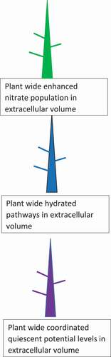
A base functionality of ETS has been developed: ETS is a transient, plant wide system wherein 1) nitrate ions are putatively absorbed by a variety of epidermal structures including trichomes and transferred into the extracellular region, 2) hydrated pathways are produced in the extracellular region through which these nitrate ions pass 3) electrical potential gradients are created in the extracellular region which provide a force field to provoke movement of nitrate ions through these pathways. Anthropomorphic climate has three dimensions: light, temperature and moisture. Phytomorphic climate has five dimensions: light, temperature, moisture, earth tides and atmospheric ion presence. ETS is a natural adaptation of plants to the transient nature of atmospheric negative polarity ion presence. It provides a mechanism for plants to utilize this ubiquitous and renewable source of nitrate.

Introduction

Figure 1–2. The global electric circuit is a loop of moving electric charges between the electrosphere and the earth’s surface and from the earth’s surface back to the electrosphere.^{1, page 31} This loop of charge movement has two directions. Under fair weather positive charges move downward from electrosphere to the earth’s surface. Under disturbed weather, negative charge moves downward from the electrosphere to the Earth's surface. Figure 1 illustrates this loop of bidirectional charge movement.

Figure 1. Ion movement due to the global electric circuit and the marine layer. The global electric circuit is a loop of ion movement between the electrosphere and the land mass. The marine layer is mass of ions moving inland from the ocean to the coastal land mass. These ions can be positive or negative polarity.

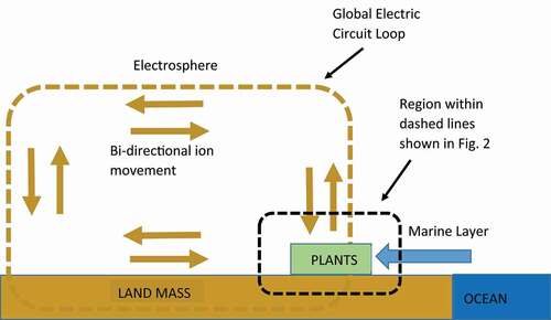
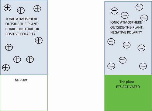
Figure 2. Two possible polarities of ions surrounding the plant. The global electric circuit and the marine layer bring positive or negative polarity ions into the atmosphere surrounding the plant. When the plant senses that the atmosphere surrounding it contains negative polarity ions, it activates a plant wide system (ETS) to absorb and utilize these negative polarity ions.

The marine atmospheric layer moving inland from the coast also carries charge to the coastal regions. A prominent example of this is the Salinas Valley in California. With great regularity, this marine layer moves inland from Monterey Bay and envelopes the lower Salinas Valley with a layer of electrical charge. Figure 1 also indicates this movement of charge.

In both the global electric circuit and the marine layer, the focus of interest is within the dashed region illustrated in Figure 1. The electrical charge fills the atmosphere surrounding plants at the soil surface. The polarity of this charge can be positive or negative. Figure 2 illustrates this distinction in the polarity of the ions in the atmosphere. The ions act as a stimulus. Plants respond differently depending on the polarity of the ions. If the polarity of the ions is positive, the plant does not respond. If the polarity is negative, there is a plant wide response. This difference in response leads to the following hypothesis:

In the presence of negative polarity atmospheric ions plants activate a plant wide system to absorb and utilize these negative polarity ions.

This plant wide system, termed the Extracellular Transport System (ETS), is present in all tissues involved in nitrate absorption, transport, reproduction and storage. Verification of the hypothesis will be presented in three parts depending on the location of the nitrate ion:

• Location I: In the atmosphere outside the plant,

• Location II: In the interfacial volume. The term “interfacial volume” is defined herein as the region above the plant surface which contain structures and/or an E field which can cause significant enhanced absorption of atmospheric nitrate ions.

• Location III: Inside the plant.

The focus will be on movement of the nitrate ion in each of these locations.

It is also possible to visualize this hypothesis in terms of a stimulus/response mechanism wherein negative polarity atmospheric ions are a stimulus and the activation of ETS is a response.

Negative polarity atmospheric ions are dominated by forms of nitrate ions.^{1,page 33} The term “negative polarity ion” is assumed to be nitrate ions throughout this paper.

All time references in this paper are in Pacific Standard Time.

Limitation of the hypothesis

The hypothesis concerns the existence and functionality of a plant wide system (ETS) for atmospheric nitrate absorption and utilization. It does not state an anatomical location of the onset of the pathways and electric fields. This is beyond the scope of the hypothesis. The discussion which follows is limited to verifying the existence of ETS and characterizing its functionality.

Location I: Nitrate ions in the atmosphere outside the plant

Verification of the hypothesis begins outside the plant with measurement of the magnitude, polarity and timing of atmospheric ion movement to a simulated plant surface. These measurements will be illustrated in Figure 3–6.

Figure 3. Simulated plant surface surrounded by negative polarity atmospheric ions. Nitrate ions move to the plate because of the difference between the potential of the atmosphere ΦA and the potential of the plate ΦP.

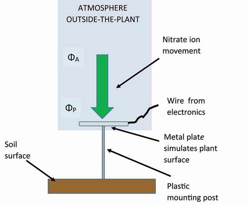
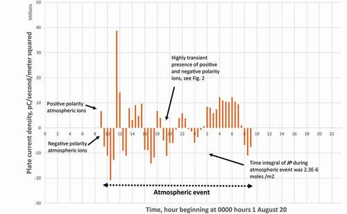
Figure 4. Atmospheric ion current density, Soledad, CA, pinot noir vineyard, 5 min data acquisition, 9 to 10 December, 2020.

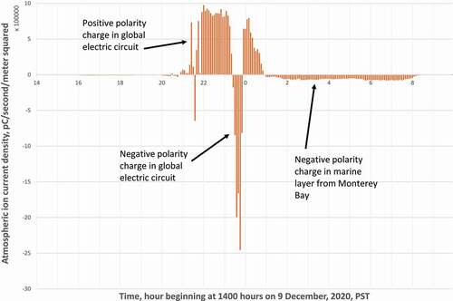
Figure 5. Soledad, CA, Vineyard, Pinot Noir, Plate ion current density, 0.25 m height, 10 August to 31 August, 2019.

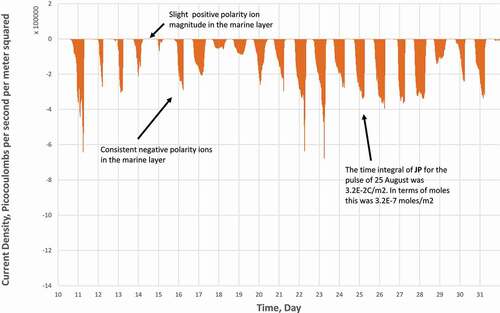
Figure 6. San Simon, AZ, Pecans, sensing plate ion current density, 1 meter height, 1 August to 2 August, 2020, 30-min data acquisition.

Simulated plant surface

A metal plate shown in Figure 3 mounted above the ground functions as a simulated plant surface. The rationale is to measure the rate of arrival of nitrate ions on this simulated plant surface. To do this the plate is subjected to a three step procedure:

Step 1: Electronics connects the plate to ground.

Step 2: Plate is disconnected from ground and exchanges charge with its surroundings. Plate potential equilibrates with the potential of the atmosphere at the height of the plate. Potential traverse recorded in electronics.

Step 3: Plate connected to electronics. Electronics sets the plate potential at ground potential. Potential difference from the atmosphere to the plate causes ion movement. Electronics draws off the charge from the plate and counts the electrons transferred. Plate is held at ground potential. Counting continues for a fixed time period. Result is the number and polarity of ions arriving at the plate in a fixed time period. Rate of ion arrival is computed by dividing the total count by the fixed time period.

This three step procedure is the same procedure employed by Wilson in 1906 using microscopes, electroscopes and a brass disc.²

The rate of ion arrival from the atmosphere to the plate can be described mathematically by a force/flow type of relation:

(1) Force * proportionality constant = Flow

In terms of the diagram in Figure 3:

(2) (Φ_{A –} Φ_P) * σ = J_P [coulomb/second/meter squared]

where Φ_A is the potential of the atmosphere in the vicinity of the metal plate in volts,

Φ_P is the potential of the metal plate held at ground potential in volts,

σ is the conductance of the path between the potentials in coulomb/second/meter squared/volt,

J_P rate of ion arrival on the plate during the atmospheric event.

The potentials and conductance are function of x, y, z, and t in units of meters and seconds. The count of electrons as a rate is given by J. The total number of electrons is given by the time integral of J. When the ions arriving at the plate surface are positive ions, the value of J will be positive. When the ions arriving at the plate surface are negative ions, the value of J will be negative. The time integral of J gives the total number of ions arriving at the plate during the entire atmospheric event. The term “atmospheric event” is defined herein as the duration of time between the onset of negative polarity ion presence and the termination of negative polarity ion presence.

Contrast between nitrate arrival rate in the marine layer and the global electric circuit, Figure 4–6

Figure 4 shows the values and polarity of atmospheric ion arrival rate or current density measured in a pinot noir vineyard with a plate mounted at a height of 25 cm at the end of a row. The current density, an electric circuit term, can be interpreted as an arrival rate of ions to the plant surface. The latter is a more physically understandable term. The term “arrival rate” and “current density” are synonymous. In Figure 4, there was a 30-min putative presence of negative polarity ions from the global electric circuit followed by a 9-h presence of negative polarity ions in a marine layer from the ocean in Monterey Bay. The arrival rate of ions in the global electric circuit is high in magnitude and short in duration. By contrast, the marine layer arrival rate is lower in magnitude but much longer in duration. The peak magnitudes of the global electric circuit pulse J_P was 2.5E6 pC/sec/m2 and 7.6E4 pC/sec/m2, respectively. The time integral of J_P in Eqn. 2 for the global electric circuit event and marine layer events were 1.4E-2 coulombs/m2 and 1.6E-1 coulombs/m2, respectively. The pattern in Figure 5 illustrates the generality of this contrast in timing and magnitude of nitrate ion arrival rate from the marine layer. The timing of the marine layer nitrate movement is set by the timing of the cold air mass movement drawn inland by the heated landmass of the coastal region. Figure 6 illustrates the generality of the timing and magnitude of nitrate arrival rate from the global electric circuit. The histogram in Figure 7 indicates the global electric circuit has the same timing as the marine layer. Negative ion presence is in general a night time phenomenon.

Figure 7. San Simon, AZ, Pecans, histogram: frequency of occurrence of negative polarity atmospheric ion current density greater than 1e4 pc/sec/m2 magnitude, 1 July TO 31 August, 2020, Thirty-minute data acquisition.

In background data sets in production agriculture blocks in Arizona and California developed over the past 2 years, the rate of arrival of negative polarity ions varied over a four order of magnitude range, from 5E3 to 5E7 pC/second/m2.

The magnitude of rate of arrival can be integrated over the duration of the atmospheric event to yield a total nitrate ion arrival in moles. This value will vary widely but is included in the comments made in Figures 4–6. The conversion from charge to moles employs the standard faraday constant of 0.94E5.^{3, Table of Physical Constants}.

Summary of the characteristics of the atmosphere as experienced by plants

The atmosphere contains ions of two polarities: positive and negative. Negative ions are forms of nitrate ions. As such they can be used in plant growth and reproductive processes. The presence of negative ions is transient. The magnitude of negative ions present varies widely in magnitude.

The system that the plant has evolved to efficiently use negative ions takes into account these characteristics. It must be plant-wide because absorption is mostly confined to the epidermis but usage and storage is in the entire plant.

The plant system will be transient because it is a transient response to a transient stimulus.

Nitrate ions are charged. Uptake from the atmosphere and transfer within the plant can employ electric force fields.

Concentrations of negative polarity atmospheric ions will vary with height. The uptake of ions by the plant will vary with height.

Nitrate from the atmosphere is renewable but the plant has no way of knowing when the presence of atmospheric nitrate ions will repeat. Uptake will occur whenever nitrate ions can be immediately stored or used. The plant has no other source of nitrate ions other than detritus.

Location II: Nitrate ions in the interfacial volume

This part of the hypothesis concerns absorption of nitrate ions by the plant. The mechanisms whereby transfer takes place will be discussed from an anatomical point of view

The wide range of nitrate movement into the plant surface and strongly different rates of movement suggests the presence of an interfacial volume between the plant surface and the atmosphere. Within this volume there are structures that function as ion attractants. Figure 8 illustrates schematically the range of epidermal structures in this volume that can contribute to nitrate uptake. Direct openings into the plant surface is largely confined to stomates.⁴ These openings are only on the plane of the plant surface or even below this plane on the case of gymnosperms.^5,6 Stomates are also covered by a cuticle which extends into the substomatal cavity. The cuticle would prevent entry but at the same time defines a path of entry of atmospheric ions. A cluster of protons at the bottom of the substomatal cavity when the guard cells open the cavity would result in an electric field which would move negative ions from the plane outside the surface into the cavity.

Figure 8. Schematic interfacial volume showing structures, putative positive charge locations (red) and electric field lines (purple) at the plant surface. The cuticle (tan) is shown covering the sides of the substomatal cavity and only the basal cells of the papillae.⁷

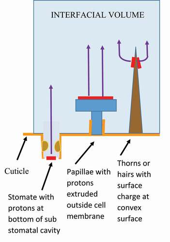
Presence of positive surface charge on these structures such as shown in Figure 8 (in red) causes movement of negatively charge nitrate ions to the structures.

The surface of plants is replete with structures which extend above the surface and can function as attractants for nitrate uptake. These structures are trichomes. Trichomes have a wide variety of form.^{4, Figs. 9.24,9.25; 6}

Trichomes composed of living cells in many cases do not have a cuticle⁷ and at the same time they extend above the plant surface. The living cells could provide direct passage of the nitrate ions into the symplast. The living cells could also extrude temporarily protons outside the cell membrane in the manner shown in Figure 8. These could provide a micro-electric field extending into the atmosphere to attract negatively charged ions.

Trichomes not composed of living cells but of highly convex shape such as thorns are locations of higher positive charge concentration. This shape makes them function as miniature lightning rods to attract the negatively charged atmospheric ions. The shape of such convex structures are in some cases almost ideal for this purpose. A particular example is the arapidosis trichome.^{4, Fig. 5.31} This shape leads to a quasi omni-directional electric field.

Epidermal structures viewed as generators of an electrostatic field, Fig. 8

It is possible to consider cellular and non-cellular epidermal structures as generators of an electrostatic field at the plant surface pointing out away from the surface. The electric field lines of force associated with these structures are shown in Figure 8 as electric lines of force moving from the structures into the atmosphere. These field lines function as nitrate ion attractants. Permanent epidermal structures such as thorns would channel nitrate ions to the plant surface. Transient epidermal activity in living cells in trichomes would provide a direct path for nitrate entry as well as a channeling function. This field would attract negatively charged nitrate ions. Ions would enter the symplast through living cells in the trichomes or stomatal openings.

Mathematically this field can be described by a positive increase in the magnitude of Φ_P in Eqn. 2 above. The increase in potential difference would increase the magnitude of J_P.

The extent of the interfacial volume above the plant surface is the distance wherein the E field generated by epidermal structures has significant influence on ion movement.

While the existence of such fields on plants has not been experimentally verified, the efficacy of the electric field has been tested. There has been a study of the atmospheric charge levels at the 3-m height under specialized conditions of no vegetation and no wind⁸. This study indicated considerable stratification. The eight plant types tested by the Author indicated that within the plant there is a consistent polarization with the upper part of the plant normally higher in potential than the lower part of the plant. This would have a considerable influence on the nitrate uptake.

There is at present no experimental support for a simulated plant surface with active characteristics.

Summary of epidermal structures viewed as ion attractants

An interfacial volume exist between the plant surface and the atmosphere. This volume contains structures that facilitate movement of nitrate ions toward the plant surface and into openings in the plant surface. The structures generate electric lines of force within the interfacial volume that function to channel nitrate ions toward and into the plant surface.

Location III: movement of nitrate inside-the plant

Introduction

The hypothesis states that a plant-wide system exist that utilizes absorbed atmospheric nitrate ions. Utilization requires the transport of nitrate ions from source to destination. ETS is essentially a nitrate transport system. Examples of nitrate transport will be presented in four crop types: corn, lemons, chili peppers and avocados. Movement of nitrate requires a pathway and a force field to provoke the movement in the pathway. In other words, the functionality of ETS must extend not only to the nitrate itself, but also to the pathway and the force field. The four examples will demonstrate functionality of ETS in three dimensions: movement of nitrate itself, existence of a hydrated pathway and existence of an electric force field to provoke movement of a charged nitrate ion.

The hypothesis states that this functionality is activated by the presence of negative polarity atmospheric ions. The examples will demonstrate this simultaneity. The major tool for this demonstration will be the simultaneous plots of patterns of atmospheric nitrate rate of arrival on the metal sensing plate outside the plant and the nitrate population, hydrated pathway and force field inside the plant. The functionality of ETS has three dimensions: the nitrate itself, the hydrated pathway and the force field within the pathway.

Over the past 2 years, the Author has made these simultaneous measurements of the atmospheric ions levels and these three dimensions in the extracellular region of the plant during periods of positive and negative polarity ion levels in the atmosphere surrounding the plants. These measurements were made in production agriculture blocks of pistachios (Pistacia vera kerman), pecans (Carya illinoinensis, western), avocados (Persea americana, haas. organic), wine grapes (Vitis vinifera, pinot noir and cabernet sauvignon), cotton (Gossypium hirsutum, pima), lemons (Citrus limon, prayer), corn (Zea mays, blue river 64N94, organic), chili peppers (Capsicum annuum, machete, organic). The measurements of atmospheric ion levels were similar to the measurements described in the previous sections. The height of the metal plate was 0.25 meters or 1 meter or both. Measurement of extracellular nitrate population, extracellular potassium population, water content and extracellular quiescent potential was made using electrochemical sensors and procedures known as the Phytogram technique. The basic characteristics of the Phytogram Technique will now be explained.

Phytogram technique

This technique senses electrochemical characteristics of the fluid in the extracellular volume within the plant. It originally began as a potential measurement within the plant similar to the potential measurements in electrocardiograms in humans. The term “phytogram” is a shortened version of the term “electrophytogram.” The Phytogram has evolved into a measurement of both physical and chemical parameters of the extracellular fluid of plants.^9-11

Application of the Phytogram has been almost exclusively confined to production agriculture. The application of the Phytogram in the context of this hypothesis will now be explained in terms of a representative plant type, corn. The sensors, technique and results are the same in other plant types. Differences arise due to the different anatomical locations of the electrochemical sensors and plant architecture.

Phytogram technique as applied in corn, Fig 9a 9e Location of the sensors in the corn plant

Figure 9a gives the location of the sensors in the corn plant. There are three sensors in the stalk and five sensors in the leaf blade collars. The leaf blade sensors are in the transfer region of the nitrate gathering leaf blades. The sensors in the nodes are located in the nitrate storage and usage regions.

Figure 9a. Sensors in the corn plant. Sensors in the stalk were noble metal filaments, 406 micrometers in diameter, 10 mm long. Sensors in the leaf blade collars were noble metal filaments 150 micrometers in diameter, 6 mm long.

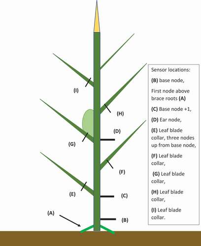
Figure 9b. Cross-sectional view of the sensor filament resident in plant tissue. Filament diameter is 406 micrometers. Average cell diameter is 20 micrometers. Extracellular fluid wets the surface of the filament. This fluid contains nitrate and potassium ions (not shown). Nitrate and potassium ions from this fluid adsorb on the filament surface. Thickness of layer shown is in the order of nanometers. Filament surface is equipotential and in equilibrium with extracellular fluid potential. Distance between filament surface and normal functioning cells is in the order of micrometers.

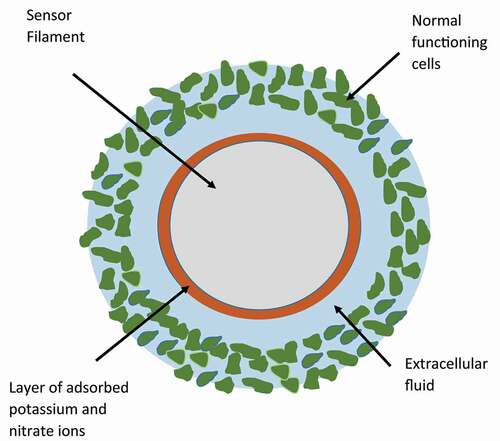
Figure 9c. Cross-sectional view of the sensor filament resident in plant tissue. Filament diameter is 406 micrometers. Average cell diameter is 20 micrometers. Extracellular fluid wets the surface of the filament. This fluid contains nitrate and potassium ions (not shown). Nitrate and potassium ions from this fluid adsorb on the filament surface. Thickness of layer shown is in the order of nanometers. Filament surface is equipotential and in equilibrium with extracellular fluid potential. Distance between filament surface and normal functioning cells is in the order of micrometers.

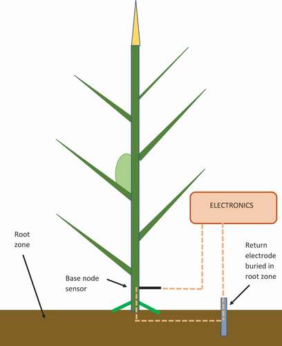
Figure 9d. Conditions in the extracellular volume when the atmospheric charge surrounding plant is charge neutral or positive polarity.

Figure 9e. Conditions in the extracellular volume when the atmospheric charge surrounding plant is negative polarity.

Implant of the sensor into the tissue

The stalk and leaf blade collars are soft tissue such that predrilled holes in the plant are not required. The filament is inserted directly into the node for the full 10 mm of sensor length. The plant responds immediately by sealing the entry point and servicing the damaged tissue.¹³ This servicing is accomplished within hours. The situation outside of the damaged tissue then functions normally. This is seen in the abnormal (but coherent and predictable) values immediately after implant and then a sequence of equilibrated values. In terms of plant physiology, this rod-like implant is similar to the rod-like implant of an aphid stylet, but the location of the filament is not within a phloem cell, but a general extracellular region of tissue.^{14, page 300; 15, page 206} The filament residence is normally one to 2 years.

In the case of hard tissue (trunks and branches) pre-drilled holes and customized nylon set screws are required to permit insertion of the filament. The electrochemically active surface of the filament is then located in the region at a smaller radius than the cambium.

In all cases, biocompatible materials are required to prevent necrosis.

The result of this implant procedure is a sensor part of which is inside the plant and part of which is outside the plant. The part outside the plant is connected to electronics. The sensor surface inside the plant functions as an “electrochemical window” from which one can observe the activity of the cells adjacent to the surface. One can initiate electrochemical procedures outside the plant which when imposed inside the plant assay the constituents of the extracellular fluid wetting the sensor surface.^{3 chapters 7 and 13; 16 chapter 7; 11, and 13}

The sensor surface inside the plant

Figure 9b illustrates the sensor (filament) resident inside the plant. The relative size of the cells and the filament are shown and stated in the Figure caption. Functionally, the surface is wetted by extracellular fluid. The extracellular fluid contains ion levels set by the physiological activity of the cells adjacent to the sensor. Some of these ions adsorb on the sensor surface and form one side of a double layer capacitor. The other side of the capacitor is a layer of charge on the surface of the metal. The sensor becomes a double layer capacitor whose charge magnitude is set by the number of adsorbed ions. The two principle adsorbed ions are potassium and nitrate. By identifying the number of nitrate ions adsorbed, one is able to quantify the number of ions in the extracellular fluid. The result is an assay of nitrate ions reported as a population of ions on the sensor surface. This is the origin of the nitrate population values reported in Figure 11, 12, 16, 17 and 18.

To convert from population on the sensor surface in nanocoulombs to concentration in the extracellular fluid in moles/liter one can employ a calibration factor based on in vitro calibration testing. The result is the concentration of nitrate in the extracellular fluid contiguous to the filament surface shown in Figure 9b.

The timing of implant is limited by the age of the tissue. It is necessary to implant only during the upper shoulder of the S curve of growth.^{14, Fig. 16.2} This avoids scar tissue formation at the sensor surface.

The electrochemical circuit

Figure 9c shows the electrochemical circuit required in the electrochemical procedures applied to the base node sensor shown in Figure 9a. The second electrode is normally a zinc rod buried at a depth outside the range of short-term penetration by irrigation water but still within highly conductive soil. This second electrode is essentially nonpolarizable.^{3, Fig. 1.3.5}

The current levels in this circuit are in the order of nanoamperes.

Regional values of Nitrate

The wetted area of the sensor may be located along the full length of the filament. The concentration is then a characteristic of the annular volume of fluid contiguous to the sensor surface. As such it encompasses the different tissue types within this annular volume. Each tissue type can contribute to the adsorbed population. In other words, the value of nitrate is a regional value. This same situation holds for the values of water content and quiescent potential. From the standpoint of ETS, the hydrated pathway and force field are also regional values of the extracellular volume.

Contrast in plant status when ETS is not activated and ETS is activated

Figure 9d illustrates the whole plant status when ETS is not activated. Figure 9e illustrates the basic parameters of ETS: nitrate population, water content and quiescent potential when ETS is activated.

ETS patterns during a twenty-two day time period in corn Figure 10–11

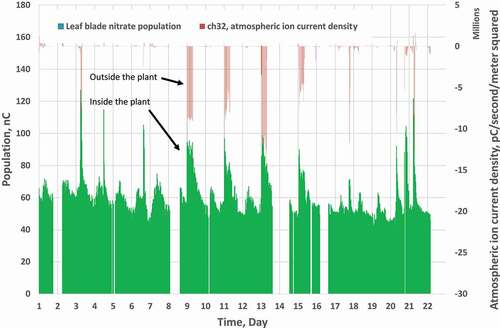
This implementation in corn will be shown in a sequence of Figures at a weekly and then an hourly time scale. First the atmospheric ions levels will be shown in Figure 10 for a 22-day period. This is the stimulus that activates ETS. Then the simultaneous atmospheric ions levels (the stimulus) and the inside-the-plant nitrate population (response) will be shown in Figure 11 for this same 22-day period. Precise timing of nitrate population, water content and quiescent potential will then be shown in the hourly time scale of Figures 12–14.

Figure 10. Pearce, AZ, Corn, Organic, blue river 65n94, ch31, atmospheric ion current density, 0.25 and one-meter height, 1 August to 22 August, 2020.

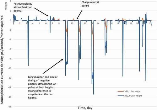
Figure 11. Pearce, AZ, simultaneous measurement of atmospheric nitrate outside-the-plant and enhanced nitrate population inside-the-plant, corn, organic, 1 to 22 August, 2020.

ETS patterns during a thirty three hour time period in corn Figures 12–14

A long duration atmospheric negative ion pulse occurred at 0000 hours on 10 August, 2020. Figure 12 shows the carryover of the nitrate population after the termination of the atmospheric pulse. This continuation or carryover is a consistent characteristic of the nitrate population for all eight crops. This indicates a short-term storage on the part of the plant that is necessary to distribute the nitrate which has been taken up. Figure 13 shows the water content shifts in the plant concomitant with the nitrate population movement.

Activation of ETS causes a shift in potential to very coordinated and definitive values. For example in Figure 14, the potential of the blade collar at the top of the stalk and the potential in the base node at the bottom of the stalk moved to the same potential level upon ETS activation. This set up a potential gradient and subsequent force field which drove nitrate into the ear node and the base node.

The dots in the patterns in Figure 12–14 are the half-hour data acquisition times. This 30-min acquisition rate is not sufficient to separate out which changes at the onset occurred first. It is possible to conclude that the activation was plant-wide. Deactivation appears to be set by the time at which the nitrate has reached its destination in reproductive or storage tissue.

The values of nitrate population are given as a number of coulombs. In vitro calibration runs in a chamber of known size containing known concentration of nitrate, potassium ions and water permitted the values of nitrate population to be quantitatively related to values of molarity of nitrate. The total amount of nitrate could not be obtained from the molarity value alone since the volume of fluid at the known concentration in vivo is not known. This will be discussed below in the discussion of ETS avocado patterns.

Transient character of ETS in lemons Figure 15

The transient character if ETS is most apparent in shifts in quiescent potential upon ETS activation and deactivation; Figure 15 illustrates this in plant wide sensors in a lemon tree. The deactivation level of the quiescent potential was about 1450 mV. Activation caused shifts as high as 1000 mV. This is probably due to the complex architecture of the lemon tree. The significant part of this shift is the return of the entire plant to the deactivation level when the nitrate ions have been dispersed. This suggests the deactivation potential level is also quite definitive.

The patterns in Figure 15 also illustrate the situation wherein a response is observed when no stimulus is observed. The reason for this is the discrete or digital nature of the stimulus and the equally discrete nature of the method of data acquisition. If 30-min recording intervals are scheduled, the electronics performs the data acquisition procedure at the beginning of the hour and half hour. Thirty plant sensors and at least one or two plate sensors are interrogated. This procedure takes 6 min. If the stimulus/response of a particular sensor occurs during these 6 min, it will be recorded. If not the electronics will record a quiescent reading for the sensor. For example, data acquisition takes place between 1000 hours and 1006 hours. The atmospheric event occurs during this time. It will be recorded. If the atmospheric event occurs between 1006 and 1030 h it will not be recorded. This mismatch is the reason for the lack of a one-to-one correspondence between stimulus and response in the patterns of Fig. 15.

ETS in chili peppers, Figs. 16a-d

A guide for examining the chili pepper patterns in Figs. 16a-c is first shown in Figs 9d and 9e. Although the plant type in Figs. 9d and 9e is corn, ETS functionality is the same for chili peppers. The following figures contain parallel patterns: Figure 12 and Figure 16a; Figure 13 and Figure 16b; Figure 14 and Figure 16c. The sensor is in the upper shoulder of the chili itself. This is the site of the termination of nitrate transfer. It is also the site of the onset of nitrate assimilation.

Figure 12. (a) The atmospheric pulse changed from zero to 10 M pC/second/m2 within a duration of thirty minutes. This approximate level was maintained 7.5 hours. Decline was equally precipitous. (b), (c), (d), (e) The base node, ear node and leaf blade nitrate population increased within the same time period. This indicates the response within the plant was systemic. The magnitudes of the increase were different. But these magnitudes are proportional to the product of the wetted area of the filament and the concentration of nitrate within that wetted area. This makes it difficult to make direct comparison of the magnitudes. (f) There was a definite carryover of the response past the end of the atmospheric ion presence. This suggests that the nitrate was absorbed by the plant and then temporarily stored to permit a slower transfer to the usage and storage locations.

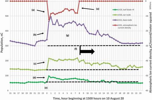
Figure 13. (a) The onset of hydration of the pathways were systemic. (b) Hydration continued past the end of the atmospheric pulse to permit transfer of nitrate to the base node. (c) Hydration of the ear node was initially enhanced but then elicited a decline below the initial level.

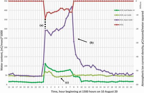
Figure 14. These quiescent potential patterns will be examined as a chronology over the duration of the atmospheric event. The graph shows patterns in the leaf blade at the top of the stalk, the ear node in the middle of the stalk and the base node at the bottom of the stalk. (a) The potential values differ between the three locations before ETS activation by 550 mV. (b) Onset of negative polarity atmospheric ions activates ETS resulting in enhanced nitrate levels (Figure 12) and hydrated extracellular pathways (Figure 13) and now in Figure 14 a shift in quiescent potential, (c) The leaf blade and base node potential are changed to 950 mV, (d) the ear node changed to 1060 mV. This results in a gradient of 110 mV between the ear node in the middle of the stalk and the base node and leaf blade at the bottom and the top of the stalk, respectively. The significant aspect of this gradient is that the ear node potential is positive with respect to the base node and leaf blade node. A negative ion in the extracellular region would be driven toward the ear node with this gradient (electrical force field). These levels suggest that ETS has set up these potential levels to force nitrate ions toward the ear node. This condition continues throughout the duration of the event. (e) When the event terminates, the potentials return to their pre-event levels.

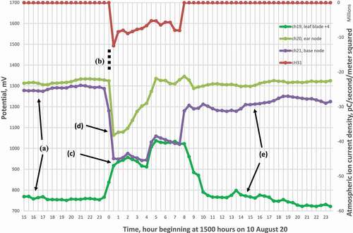
Figure 15. Soledad, CA, lemons, conventional, 1 to 12 April, 2020. (a) Potential level of widely separated parts of the plant during the ETS unactivated mode is in the order of 1450 mv relative to a zinc reference electrode in the soil. (b) ETS activation causes a consistent shift to lower potential values as great as 1000 mV, (c) Differences within the parts of the tree as high as 300 mV. These patterns suggest that in a complex plant architecture such as a lemon tree, ETS sets up a complex set of potential levels which govern nitrate movement or non-movement during activation.

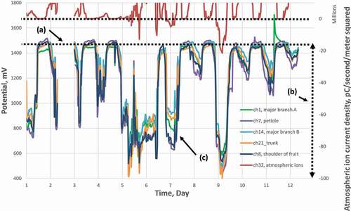
Figure 16a. Pearce, AZ, Chili Peppers, Nitrate population in the upper shoulder of the chili and atmospheric ion current density, 16–17 August 2020. (a) Single high magnitude atmospheric ion pulse. (b) Duration of transfer near constant for 9.5 h.

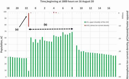
Figure 16b. Pearce, AZ. Chili Peppers, water content in upper shoulder of the chili and atmospheric ion current density, 16–17 August 2020. (a) ETS immediatley hydrates the extracellular region in the vicinity of the sensor.

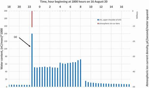
Figure 16c. Pearce, AZ, Chili Peppers, Quiescent potential in the upper shoulder of the Chili, 16–17 August 2020. (a) ETS shifts the potential first to a higher level than ambient and then to a lower level than ambient. This is interpreted as a method of permitting the chili to prepare for nitrate.

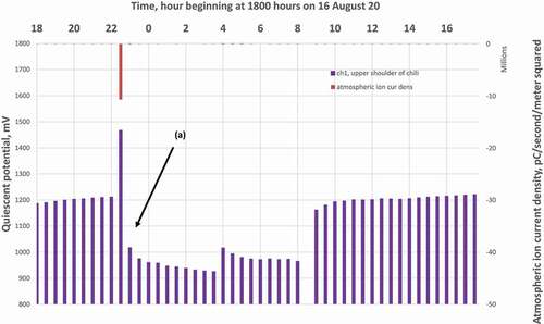
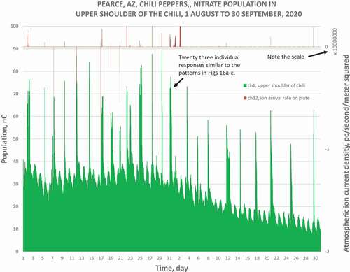
Figure 16d. Pearce, AZ, Chili peppers,upper shoulder of the Chili, 1 August to 30 September, 2020.

A single half-hour global electric circuit relatively high magnitude pulse of negative polarity ions occurred at 2230 h. The next 9.5 h had no further negative ion presence. ETS absorbed nitrate for one-half hour but then controlled the transfer to the chili pepper at a near constant rate for the next 9.5 h, presumably to facilitate steady transfer of the nitrate during growth. This illustrates plant wide controlled storage and controlled transfer at the same time.

A definite and distinct transient occurred in the nitrate population, water content and quiescent potential during the first 30 min of the response. Response was quasi steady after this first 30 min. The interpretation of this initial transient is the time required for the plant to set up reductases in the chili to assimilate the nitrate. Taiz and Zeiger refer to a 40 min period required for reductase gene formation following introduction of nitrate presence in barley seedlings.^{15, page 362} In this case nitrate was introduced at 2230 h, the plant went immediately into an enzyme production mode. Reductases were established within the chili. This took 30 min. Then transfer and assimilation were sustained for the next 9 h. ETS fed nitrate into the chili at a near constant rate as seen by the near constant pattern of quiescent potential in Figure 16c after the first 30 min.

The patterns shown in Figs 16a-c are one of twenty-three such responses over the two-month maturation period of the chili. These patterns can be viewed in the context of the long-term nitrate population shown in Figure 16d.

Nitrate movement in an avocado leaf petiole Figure 17–19

There were numerous negative polarity atmospheric ion events due to the ocean marine layer from Monterey Bay during the period February 1–29, 2020. Figure 17 illustrates the uptake of ions and subsequent transfer of these ions through the leaf petiole. The pulse-like character of the plant response followed the pulse-like character of the marine layer stimulus. Why the cluster of negative ions did not repel each other is inexplicable at this time. But the observation of a pulse shape is very decisive. The pattern in Figure 17 also indicates a non-response on the part of the plant on 20 February. This could be a result of a response in a different part of the tissue not near the sensor.

Calculation of the amount of nitrate in the atmospheric ion pattern

Figure 18 illustrates the atmospheric stimulus/plant response on an expanded time scale for 24-h period beginning on 16 February. This duration of the atmospheric event was 17.5 hours. The duration of the plant response was 12.5 hours. These simple patterns and the simple physical location of the sensor in the petiole permits a determination of the amount of atmospheric nitrate and the amount of nitrate passing through the petiole.

The determination is implemented by dividing up the pattern of atmospheric nitrate into a sequence of 30-min segments. The average arrival rate of nitrate collected on the plate for about 5 s during the 30 min is assumed to be the same value for the arrival rate during the entire 30-min period. The amount of nitrate arrived during the 30 min is this value times 1800. The amount of nitrate arrived during the entire atmospheric event is the summation of the nitrate arrived during each of the 30-min segments of the event, The result of this computation for the amount of nitrate arriving at the plate during the atmospheric event is 4.6E10 pC/m2. This converts to 4.6E-7 moles/m2 of nitrate ions.

Calculation of the amount of nitrate in the population passing through the leaf petiole

The method employed in the calculation of the total amount of nitrate ions passing by a cross section of the petiole is to divide the total time period of the population passage into 30-min time segments. Each segment is characterized by three values: concentration of the nitrate during the 30-min time period, length of the cluster during the 30-min time period and cross sectional area of the cluster during the thirty minute time period. The total amount of nitrate moving through the extracellular wetted area of the petiole cross section is then given by the following

(3) Total amount of nitrate = Σ c_i * d_i * A_i

where the summation Σ is over the ith segments of the nitrate population response during the event in units of moles and

c_i is average concentration during the i_th segment[moles/m³]

d_i is the average length during the i_th segment [m]

A_i is average cross sectional area during the i_th segment [m²]

Incremental concentration is the concentration increment above the base level of concentration just before the beginning of the event. Eqn. 3 is a method of digitizing an analog event measured at discrete intervals.

Before applying Eqn. 3 to the patterns shown in Figure 18 it is better to apply Eqn. 3 to a theoretical wave or cluster passing by the cross section of the petiole which contains the sensor. Figs 19a and 19b are presented to enhance understanding.

Fig. 19a shows a wave or cluster of nitrate ions passing through the petiole. This pulse-like form was observed in avocado, wine grape and cotton petioles. The mathematical approach is to divide the cluster into time segments and determine the amount of nitrate passing the cross section during each time segment. The dimensions of the variables in Eqn. 3 provide insight into the method. Length times area yield a volume. Then concentration within this volume yields an amount of nitrate contained in the volume.

An alternate explanation is that concentration is an intensive variable. An amount of nitrate is an extensive variable. Eqn. 3 makes the conversion from an intensive variable to an extensive variable.

Fig. 19b gives an example of nine time segment having different values of concentration, length and area

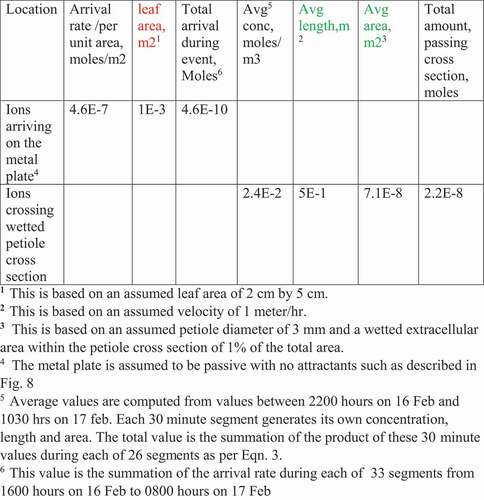
With this rationale in mind Eqn. 3 can be applied to the pattern of nitrate moving through the avocado leaf petiole. First the ith population in nanocoulombs was converted to a concentration value in moles/liter using the calibration equations determined in the in vitro calibration procedures. The ith values of concentration were converted to moles/m3. Then Eqn. 3 was applied to yield a total amount for all thirty three thirty minute segments. Assumptions had to be made concerning the length of the nitrate cluster passing by the cross section of the petiole containing the sensor and the wetted area of extracellular volume. Figure 20 gives the result of this procedure.

Figure 20 gives the values of the amount of atmospheric nitrate per unit area that arrived on the metal plate during the event and the amount of nitrate passing by the cross section of the wetted area of the extracellular volume of the petiole. Figure 20 also contains representative assumed values of the leaf area, cluster velocity and wetted extracellular area in the petiole cross section.

Energy aspects of this movement of nitrate through the petiole

The amount of energy required to move the amount of nitrate in Figure 20 through the petiole can be theoretically determined if one assumes a potential gradient of 100 mV to force movement of the nitrate between the bounds of the potential gradient. The energy expended then becomes

(4) Electrical transport energy = charge * potential gradient [joules]

(5) Electrical transport energy = 7.5E-2 coulombs * 0.1 volts [joules]

= 7.5E-3[joules]

This is the transport energy required by ETS.

When the nitrate reaches its destination, it can be presumed to be converted into nitrite as a first step in assimilation. One NADPH molecule is required for one NO₃ molecule.^{15, Eqn 12.1} Assume 220 kj/mole as the energy content of NADPH. ^{15, page 226}. The energy required for the initial metabolic process

(6) Metabolic Energy = 7.5E-7moles * 220 kJ/mole = 1.65E-1 [joules]

The ratio of the metabolic energy to transport energy is 1.65E-1/7.5E-3 or 22. Hopefully, one would expect the ratio to be much greater than one. The value of 22 is in the right direction but only as valid as the assumptions made. But it does suggest that a computation of this ratio is possible and can give insight into the energy level of ETS induced movement.

Summary of Location III, movement of nitrate within the plant

Nitrate utilization is manifest in nitrate movement from multiple sources to multiple destinations within the plant. In corn this utilization is manifest in movement of nitrate from multiple leaf blades to the bottom of the stalk and the ear node. This movement is possible because of the transient presence of hydrated pathways in the extracellular volume. This movement is facilitated by electric force fields within the extracellular volume which push or pull negatively charged nitrate ions.

This movement occurs over the entire plant.

This movement is transient. The duration of movement is from the onset of nitrate ions in the extracellular volume to the arrival of the nitrate at its destination.

Movement of nitrate requires three characteristics: the nitrate ions themselves, the hydrated pathway and the force field within the pathway. ETS has all three characteristics but in addition ETS has the ability to regulate onset, storage and transfer.

The focus of Parts II and III was to verify the existence of ETS in terms of an exposition of its basic characteristics. These are enhanced nitrate population, magnitude of the hydrated pathway and magnitude of potential gradients.

Discussion

Existence of ETS

From a paleobotany viewpoint one would expect plants to have evolved using atmospheric nitrate. Prior to farming in the last several thousand years, it was the only source of nitrate outside of rainfall and detritus. This would explain the strong response to atmospheric nitrate by plants which have ample quantities of anthropogenic nitrate in the soil.

Trichomes are ubiquitous and have an extremely wide variety of shape. Assuming evolution is an adaption to a more favorable condition, the sheer variety of shape, mostly convex, would suggest plants have attempted to maximize nitrate absorption.

Electric force fields

Since nitrate is electrically charged, it seems logical that the plants would evolve an electric field mechanism for transfer. Plants make good use of protons for generation of potential sources.¹² The presence of an electric force field is an essential part of ETS.

ETS in the presence of anthropogenic nitrate input

Modification of ETS in the presence of anthropogenic nitrate input was observed in pecans and pistachios. High magnitude spontaneous positive potential pulses were observed. The problem is the location of storage of excess nitrate within the plant. Since ETS is plant wide, it was able to sense this stored nitrate. Further discussion is outside the scope of the hypothesis.

Computation of the amount of absorbed nitrate

In computing, the amount of nitrate passing a cross section of a petiole assumptions were required. This points out the inadequacy of the existing data sets. The basic problem is the sensor acquires the magnitude of the presence of nitrate at a given time. Velocity of nitrate or the derivative of presence at that same time is needed. This can only be obtained from multiple sensors in the same pathway.

The wetted area of the sensor surface can be employed as a measure of the nitrate cluster cross-sectional area. But this must be further tested.

Origin of the hydrated pathways and potential gradients of ETS

The hydrated pathways in the extracellular volume came from an extrusion of potassium ions in the cells located in the extracellular volume. This was measured but not reported because it was considered ancillary to the main characteristics of ETS. This suggests that ETS has the ability to influence the characteristics of the symplast of these cells. The shift in potential values upon ETS activation requires a shift in charge levels outside cell membranes. This also suggests ETS has the ability to influence the characteristics of the symplast of cells. Further discussion of this mechanism and anatomical origin of shifts in potential values is outside the scope of the hypothesis.

Simultaneity of changes in ETS parameter values

Acquisition of data at 30-min intervals indicates simultaneity in changes of ETS parameters at that time resolution. The patterns in Figure 15 indicate the lack of a one-to-one correspondence between stimulus and response. But there is also evidence, particularly in chili peppers, that pulses of atmospheric nitrate occur at shorter time periods. This leads to the conclusion that data must be acquired at time intervals less than 30 min to properly observe the stimulus/response mechanism.

Climate

The problem of data acquisition interval is part of a more general problem. Anthropomorphic climate, that is, climate as experienced by humans, is comprised of three variables or dimensions: light, temperature and moisture. These are analog or continuum variables. Phytomorphic climate, that is, climate as experienced by plants, is comprised of five variables or dimensions: light, temperature, moisture, ion presence and earth tides. The first three are the same as in anthropomorphic climate. But the fourth variable, ion presence, is not an analog or continuum variable. For example, in Figures 17 and 18 the atmospheric event occurred over a 17.5-h interal. This was readily recorded with a 30-min data acquisition interval. But employing 5-min data acquisition intervals, a high magnitude atmospheric event was observed in the pattern in Figure 4 with a duration of less than 5 min. The ion presence event is an analog variable within itself, but when it occurs is a discrete, non-analog variable. This must be taken into account in any acquisition procedure and also in any computation of the total amount of nitrate uptake by the plant. Earth tides are outside the scope of this discussion.

Figure 17. These two patterns are from a sensor in the petiole of a pinnate leaf of an avocado tree and the sensor of ion arrival on the atmospheric ion sensor plate. (a) Low magnitude, long duration and onset time of nitrate presence indicate these are marine layer pulses of nitrate, (b) A cluster or wave of nitrate ions passes by the sensor over a period at least seven hours, (c) No response due to this pulse. This indicates ETS is selective, (d) Figs. 18 and 19 are concerned with this period of time.

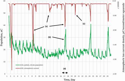
Figure 18. Same patterns shown in Fig. 17 but at an expanded time scale for the period from 1500 hours on 16 February to 1730 hours on 17 February, 2020. (a) Duration of the atmospheric event was from 1630 hours on 16 February to 0800 hours on 17 February. (b) Duration of the nitrate population wave passing by the sensor was from 2230 hours on 16 February to 1030 hours on 17 February, 2020, (c) Carryover of the plant response after the termination of the atmospheric pulse was similar to corn, See Fig. 12–14 (d) Division of pattern into 30-min segments of time. Three segments are shown here in the vertical lines in the figure. The average population value during the thirty minutes is converted to a nitrate concentration in the extracellular fluid in unit of moles/m³. A very graphic analogy to this model is a loaf of bread cut into individual slices. Each slice is a period of time.

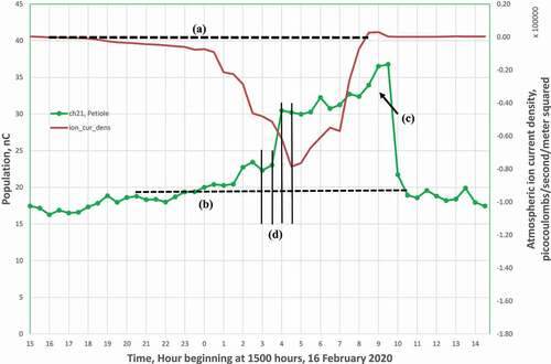
Figure 19. (Upper) Schematic space pattern of the wave or cluster of nitrate ions moving through petiole of an avocado tree leaf similar to that shown in Fig. 18., Soledad, CA, 16-17 February, 2020. (a) Petiole, side view (light green), (b) Wave or cluster of nitrate ions (white), (c) Sensor in the petiole (red). This sensor yielded the pattern of nitrate population shown in Figs. 17 and 18, (d) Electric force field pulling nitrate cluster through the hydrated pathway (purple) (e) Cross section of the petiole (black dashed line). The movement of the cluster is broken into time segments described in Eqn. 3. The amount of nitrate passing by the cross section during each time segment is the product of the three variables in Eqn. 3. The summation in Eqn. 3 is the addition of this product for each time segment

(Lower) Schematic illustration of nitrate segments that have passed by the cross section in the petiole shown in Figure 19a. (a) Petiole, (c) Sensor in the petiole, (e) Cross section of the petiole. These are a sequence of nine nitrate population time segments. Each segment has its individual value of incremental concentration during that segment, length during that segment and area during that segment. Incremental concentration is shown in the color of the segment, the horizontal length of the segment is the distance traveled during the time segment and the vertical width is the area of the cluster during that time segment. Each of these three variables can change during each time segment.

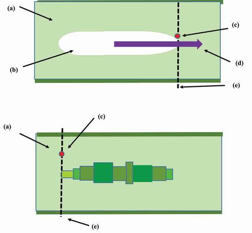
Figure 20. Amount of nitrate arriving on the metal mounted at one meter height during the event and amount of nitrate passing a cross section within a petiole during and after the event. Avocados, Soledad, CA 16-17 February, 2020. Assumed parameters are in red and green.

Correlation is not causality

The onset of the presence of atmospheric negative polarity ions consistently correlated very closely with the onset of the shifts in ETS characteristics inside the plant at a 30-min time resolution. The termination of the atmospheric pulse did not correlate closely with the termination of the ETS parameters within the plant.¹⁶ The internal ETS parameters consistently terminated later than the termination of the atmospheric pulse. This suggests very strongly that these patterns are indicative of a stimulus/response mechanism wherein the response, that is, the internal transport of nitrate requires more time to reach destinations within the plant. In other words, the absorption of nitrate is rapid, but the dissemination of nitrate is slower.

…the seed sprouts and grows, though he does not understand how - Mark 4,27

Additional information

Funding

This work was supported by the Agricultural Electonics Corporation [1].

References

- MacGorman, Rust WD. The electrical nature of storms. Oxford University Press; 1998.
- Wilson CTR. On the measurement of the earth-air current and on the origin of atmospheric electricity Proc. Camb Philos Soc. 1906;13:1–21.
- Bard AJ, Faulkner LR 2nd Edition 2001. Electrochemical Methods, Fundamentals and applications. New York: Wiley
- Evert RF. Esau’s Plant Anatomy. 3rd Edition. New York: Wiley; 2006.
- Esau K. Anatomy of Seed Plants. 2nd Edition. New York: Wiley. 1977.
- Payne WW. A glossary of plant hair terminology. Brittonia. 1978;30:239–255. doi:https://doi.org/10.2307/2806659.
- Fahn A. Structural and functional properties of trichomes of xeromorphic plants. Ann Bot. 1986;59:631–637. doi:https://doi.org/10.1093/oxfordjournals.aob.a087146.
- Crozier WD. Atmospheric electrical profiles below three meters. Journal of Geophysical Res. 1965;70:785–792. doi:https://doi.org/10.1029/JZ070i012p02785.
- Gensler WG. Electrochemical healing similarities between animals and plants. Biophys J. 1979;27:461–466. doi:https://doi.org/10.1016/S0006- 3495(79)85230-3.
- Gensler WG. (2010) Method and apparatus for determination of ion population and type of ion within plants. US Patent #8,289, 035
- Gensler WG. (2017) Method for measuring the amount of extracellular fluid surrounding a surface disposed within a plant and the ionic population and identity of the dominant ion within that fluid. US Patent 9,719,952
- Gensler W. A hypothesis concerning callose. Plant Signal Behav. 2018;14(1):1548878. doi:https://doi.org/10.1080/15592324.2018.1548878.
- Rugenstein SR. Tissue response to palladium microprobe, as observed in Gossypium hirsutum L. (Malvaceae) American J Botany. 1982;69(4):519–528. doi:https://doi.org/10.1002/j.1537-2197.1982.tb13287.x.
- Jensen, WS and FB Salisbury (1984) Botany, 2nd Edition. Belmont (CA): Wadsworth Publishing Company; 1992.
- Taiz L, Zeiger E. Plant Physiology. Sinauer Associates Inc; 2002.
- Bockris, J O’M, Reddy, AKN. Modern Electrochemistry Vol. 2, New York: Plenum Publishing Corporation; 1972.