Registration of AFM and SEM Scans Using Local Features

Abstract

Surface investigations combining the atomic force microscope and scanning electron microscope benefit from the complementarity of both technologies. For the analysis and visualization of a pair of corresponding scans, identifying their spatial alignment is essential. This article presents an automatic registration scheme based on finding correspondences between local image features. The result is then refined by maximizing a similarity measure between the aligned scans. Two feature extraction algorithms have been integrated and tested: Scale-invariant feature transform and speeded-up robust feature. For the experimental evaluation, five types of sample objects showing a variety of different surface structures have been used. The registration scheme succeeds in all application scenarios.

Keywords:

• alignment
• local features
• microscopy
• multi-modal registration
• performance evaluation

NOMENCLATURE

A, B	=	detected regions
C(x, y)	=	ground level for AFM scans
D(x, y, σ)	=	DoG detector
e rms	=	root mean square transfer error
G(x, y, σ)	=	Gaussian smoothing kernel
	=	Hessian matrix
I(x, y)	=	intensity image
k	=	parameter for DoG detector
L(x, y, σ)	=	scale-space representation with Gaussian smoothing kernel
MI(I 1, I 2)	=	mutual information of two intensity images
P I1 and P I2	=	scan histograms
P I1I2	=	joint probability
R	=	rotation matrix
S	=	scaling matrix
t	=	translation vector
T(x, y)	=	transformation model used for registration
α ij	=	coefficients for AFM ground level fitting
δ1 and δ2	=	displacement errors
ϵ S	=	overlap error in %
θ	=	rotation angle of T(x, y)
σ	=	smoothing parameter for G(x, y, σ)
ω	=	region of interest for transfer error computation

1. INTRODUCTION

The atomic force microscope (AFM) is a special form of the scanning probe microscope. In contrast to the scanning tunneling microscope, which is based on the measurement of a tunneling current between probe and sample, the AFM does not require a conducting or semiconducting sample (Binnig et al. 1986). The AFM probes the sample surface with the tip of a cantilever. From the deflection of a laser beam pointing at the cantilever, the force between the tip and surface is derived. An alternative method of measuring the cantilever bending uses piezoresistive elements integrated into the cantilever. Generally, three modes of AFM operation can be distinguished based on the tip-sample interaction: contact mode, intermittent contact mode, and non-contact mode. Besides the ability to reconstruct the specimen topography, the AFM can also be used to measure physical properties of a sample surface. These include magnetic and Coulomb forces, friction, and chemical interaction.

The scanning electron microscope (SEM) generates an electron beam that is used to scan the sample surface (Reimer 1998). An electron gun equipped with a tungsten filament or a field emission gun is used as an electron source. From the electrons emitted by the sample, a signal can be measured that is used to form an image. The resulting SEM image displays a mixture of different types of image contrast. Contrary to AFM, a pure representation of the specimen topography by image intensity is difficult in the SEM. Because the electron beam does not only interact with the specimen surface but also with subjacent material, the measured signal is influenced by the three-dimensional structure of the specimen. The imaging modes of the SEM can be distinguished depending on the type of the detected signal. The secondary electrons emitted by the sample are the most frequently used source of signal. Secondary electron (SE) scans are strongly influenced by the specimen topography. From the primary electrons that are backscattered from the sample, the backscattered electron (BSE) signal can be detected. These images are mostly influenced by the material composition of the sample.

Combined AFM and SEM studies can provide a thorough view of a specimen surface and material properties. Dual studies have been reported in several applications, indicating a clear benefit of the side-by-side use of AFM and SEM. Some examples are human hair analysis (Poletti et al. 2003), imaging of Bacillus spores (Tarasenko et al. 2006), nanofibres (Wei et al. 2008), and studies on porous anodic alumina (Zhu et al. 2010). An example of an AFM and SEM image pair can be seen in Figure 1. The AFM can provide a higher vertical resolution than the SEM, ranging down to < 0.5 Å. With a number of precautions, true atomic resolution is possible with the AFM. The maximal lateral resolution of AFM and SEM is approximately equal and falls in the range of a few nanometers. On the other hand, SEMs can be operated at low magnifications with a field of view of several millimeters. The largest AFM scans typically cover an area of 100 µm × 100 µm. Due to the high depth of field of the SEM, which can be in the range of millimeters, it can image rough surfaces. The imaging height of the AFM is limited by the vertical range of the scanner, which is typically <20 µm.

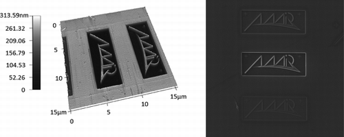
Figure 1 Example of AFM and SEM image pair, showing FIB-milled structures on a silicon wafer. The left scan shows the AFM topography view. The right scan shows a secondary electron SEM image, covering a larger scanning area than the AFM scan.

Due to the complementary nature of AFM and SEM in regard to maximal resolution and field of view, combined studies do not only benefit from successive but also from simultaneous AFM and SEM imaging. In this case, the SEM also helps to guide the AFM cantilever to the designated location. Some effort has been made towards the integration of an AFM inside the vacuum chamber of the SEM (Joachimsthaler et al. 2003; Mick et al. 2010), where the focus has been on the mechanical setup. In (Wortmann 2009), the aspect of combined AFM and SEM has been discussed under the viewpoint of visualization. The problem of finding the spatial correspondence between these imaging modalities is a widely unstudied topic. This procedure is referred to as image registration. In Seeger (2004), a method based on manual labeling with an automatic refinement has been reported. The goal of this work is to provide a fully automatic procedure for the registration of AFM and SEM scans. This can be employed for either retroperspectively analyzing the outcome of a combined AFM and SEM study, or for guiding successive AFM scans during the examination. The results must be applicable to hybrid AFM and SEM setups, as well as successively acquired scans from separate devices.

The remainder of this article is structured as follows: Section 2 describes the design of the registration procedure. A set of performance criteria is stated in Section 3 and applied for the evaluation of the registration scheme in Section 4. Section 5 provides a discussion of the results and future steps.

2. SYSTEM DESIGN

The task of image registration is a well-studied topic with its origin in the analog time of image processing. Nevertheless, no superior method for all image registration tasks could be identified as of yet. This is mainly due to the different assumptions made for specific registration problems, such as natural photograph stitching, multimodal medical image fusion, or multispectral image fusion (Zhou and Omar 2009). Although there is no generally valid solution for all image registration tasks, a procedure for image registration can be designed systematically for a given problem (Goshtasby 2005). Registration schemes can be classified under various aspects. An important means of differentiation is the classification into feature-based and area-based registration.

	Feature-based methods try to identify discriminative local image features and to determine feature correspondence between the images. In medical image registration, there is also a distinction between features artificially added to the image scene (extrinsic registration) and those directly available from the anatomy (intrinsic registration).
	Area-based methods align the images using an initial guess of the transformation function and then optimize an image similarity measure by modifying the transformation parameters. Very accurate results can be expected but the radius of convergence is small.

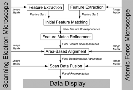
AFM and SEM image registration requires a registration scheme for multi-modal registration, which can also work with little or no prior knowledge about the transformation parameters and can handle a high amount of sensor noise. The usage of extrinsic image features is difficult and generally not wanted. Due to the large search space, the direct use of an area-based method in combination with an exhaustive search is not always applicable. Instead, a multi-stage procedure is proposed here, and the process is depicted in Figure 2. It performs a feature-based AFM and SEM image registration first. The result is then refined by an area-based method. A concrete selection of algorithms will be discussed in detail in the following.

Figure 2 Overview of proposed registration scheme. Initially, local features are extracted from the SEM and AFM scans. The features are matched against each other and the match is checked for consistency in a refinement step. Based on the feature correspondence, the transformation model parameters are computed. Area-based fine alignment is performed optionally. The final fused view is generated and then displayed.

2.1. Transformation Model

The description of the spatial correspondence between AFM and SEM scan requires a transformation model T. For any image coordinates (x, y) in the base image, T(x, y) are the image coordinates in the image to be registered. The goal of the following steps will be to determine the model parameters.

Generally, T can be any function. In some applications of image registration it is chosen to be a polynomial function or even a piecewise defined nonlinear function. These transforms are incorporated in order to correct for image distortions. However, distortion compensation can also be regarded as a step of preprocessing. The only correction applied here is fitting of a polynomial curve, in order to assure a uniform ground level in the AFM scans. The curve, as follows

has been fitted into the ground regions and subtracted from the original scan data. Additionally, the method proposed in (Gnieser et al. 2009) could be used to compensate for local distortions in the SEM scan. Similar to Fan et al. (2006), where a linear model is used to register contact and intermittent contact mode AFM scans, the transform is chosen to be a combination of scaling S, rotation R and translation t.

where

The model parameters S, R, and t are estimated from a set of automatically labeled landmark pairs. For the conformal transform model, two pairs of landmarks are theoretically sufficient to determine the model parameters. More accurate estimations are obtained by selecting >2 landmark pairs and performing linear regression.

2.2. Feature Extraction

Selecting a method for the detection of meaningful features from image scenes is one of the most critical points in the design of a registration scheme. Not only are assumptions regarding the imaging properties made here, but also about the image contents. This is critical, because the registration scheme should work with a large number of specimen and application scenarios. For example, a formerly presented application specific object detector (Wortmann and Fatikow 2009) detects carbon nanotubes exploiting their straight line property. Those objects might serve as local image features for registration purposes, but the detector requires objects of a particular shape.

When little or no knowledge about the image contents is available, local feature detectors, which are generally applicable, can be considered. Two modern approaches will be investigated here, the scale-invariant feature transform (SIFT) (Lowe 2004) and the speeded-up robust feature (SURF) (Bay et al. 2008). Both methods have their origin in monomodal applications such as image retrieval or image stitching, mainly in natural photography. Up to now, there are only a few applications of SIFT and SURF in microscopy. Image stitching for light microscopy using SURF has been demonstrated (Wortmann 2010) recently. Because preliminary investigations indicated promising results for a number of applications of AFM and SEM registration, SIFT and SURF are further pursued here. Both algorithms provide a means of interest point detection and also an interest point descriptor.

The goal of interest point detection is the identification of highly distinct image points. Those points are mainly image corners or blob-like structures. Detection is carried out in scale space, which means that the search is performed in several smoothed and downscaled copies of the image data. The SIFT algorithm uses the Gaussian smoothing kernel with the scale-space parameter σ. For an input image I(x, y) the scale-space is defined by the following function:

with the Gaussian smoothing kernel

In theory, the interest point detection of SIFT relies on the Laplacian of Gaussian (LoG) operator, which is based on second order derivatives of the image neighborhood. Practically, the LoG is approximated by the Difference of Gaussian (DoG) detector, which is computationally more efficient.

k is a constant factor separating two close-by scales. The SURF detector is based on the Determinant of Hessian (DoH) and also relies on second order derivatives:

Practically, the smoothing kernel is approximated with the help of average filters. Average filters can be computed at constant time using integral images, and therefore bring a tremendous speedup in contrast to the Gaussian smoothing kernel. The integral images are also used to compute local approximations of the derivatives.

The DoH detector produces the strongest responses on blob-like structures and ideally does not respond along edges. In contrast, the DoG is an edge emphasizing filter. Interest points along edges are undesirable, because their location is expected to be unstable. Therefore, the SIFT detector implemented a suppression of edge responses by also approximating the Hessian matrix around local extrema of the DoG.

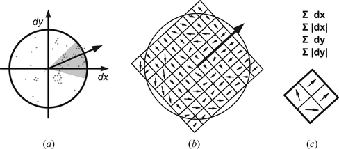
For each local feature point, a distinctive descriptor is required in order to establish feature correspondence. The construction of the descriptor is depicted in Figures 3 (SIFT) and 4 (SURF). Initially, a dominant direction is assigned to each feature point, assuring invariance to rotation. SIFT also allows multiple dominant directions by assigning multiple descriptors to a single feature point. A description vector of the local neighborhood is generated by orientation histograms (SIFT) and sums of Haar wavelet responses (SURF), each with respect to the assigned direction. The SURF algorithm enables computation of the local sums based on absolute values or separately split-up by sign. This results in a descriptor length of 64 or 128, respectively. For the SIFT algorithm, only the standard descriptor with a length of 128 has been used here.

Figure 3 Generation of the SIFT descriptor. Initially, local gradient magnitudes and orientations in the neighborhood of a feature point are weighted with a Gaussian window centered at the feature position. From the result an, orientation histogram (a) is computed, For all orientations with a magnitude of > 80% of the highest peak (indicated by the circle), a descriptor is assigned. Therefore, a grid (b) is placed around the feature point and local gradient magnitudes and orientations with respect to the assigned direction are computed and weighted by a Gaussian window. (c) From the gradients in each sector of the grid, an orientation histogram is computed.

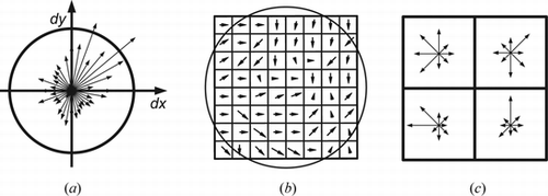
Figure 4 The SURF features descriptor. Wavelet responses for the x any y directions are computed in the neighborhood of a feature point and weighted with a Gaussian window centered at the feature position. The feature orientation is assigned with the help of a sliding window (a). A grid of wavelet responses relative to the assigned feature orientation (b) is then used to compute a descriptor entry. The descriptor entry for each block (c) is built of the sum and the sum of absolute values of the local wavelet responses. Finally, the SURF descriptor is composed out of all block entries.

2.3. Feature Matching

By establishing the feature correspondence between the AFM and SEM feature set, the spatial transformation parameters can be estimated. Generally, feature correspondence can be determined by a nearest-neighbor search using the invariant descriptor vectors. However, no algorithm is known for solving the exact nearest–neighbor problem in high-dimensional space, which is faster than exhaustive search. The best-bin-first algorithm (Beis and Lowe 1997) is a common approximation of the nearest-neighbor search, which gives a speedup by about two orders of magnitude. Also, unstable feature matches where the nearest neighbor distance is too close to the second-nearest-neighbor distance are excluded. The approximation brings the risk of not finding the exact nearest-neighbor. On the other hand, even for true nearest-neighbors there is no guarantee for feature correspondence, especially if an ambiguous image structure is present in the scene.

For the elimination of incorrect feature matches, the random sample consensus (RANSAC) algorithm is applied (Fischler and Bolles 1981). Up to now, only the invariant feature descriptor has been used to establish feature correspondence and the feature location has been neglected. RANSAC checks the initial set of matched features for consistency with the transformation model. In each iteration, a subset is randomly chosen from the initial set of feature matches. The subset has the minimal size necessary for computing the transformation model parameters. All remaining feature pairs are then checked for geometric consistency with the model parameters derived from the subset. A feature pair is referred to as an inlier, if it fits with the transformation model within the limits of a given error threshold. The inliers form a geometrically consistent set: the consensus set. Finally, the transformation parameters are computed by linear regression from the consensus set with highest cardinality over all iterations. RANSAC extensions such as m-estimator sample consensus (MSAC) or maximum likelihood sample consensus (MLESAC), define a loss function also for inliers or fit a combined error model to inliers and outliers.

There have been some attempts to further improve the initial matching by focusing on the assumption of a fixed difference in scale (Bastanlar et al. 2010). Given an initial set of feature pairs, the ratio between detected scales will cluster around the scaling ratio of the corresponding scans. This is exploited by eliminating matches with a ratio of scales deviating too much from this assumed scaling ratio. However, this ranks one aspect of the geometrical consistency check (scale) over the others (rotation and translation), whereas RANSAC checks all components simultaneously. On the other hand, for the registration of AFM and SEM scans prior knowledge about the transformation parameters is often more comprehensive than, for example, in natural photography. In most cases, the equipment provides a more or less accurate estimate of the pixel width in physical units and therefore the difference in scale can be concluded. In an SEM-integrated AFM (Mick et al. 2010), typically the difference in orientation between the AFM cantilever and SEM scanning grid is restricted or fixed. In contrast, for successive examinations with changes in the sample mounting the rotation is typically unknown.

The different amount of prior knowledge about the transformation parameters can be taken into account by implementing a post processing of the initial set of feature matches. Correspondences of features are checked for their ratio of scale and difference in orientation, and these parameters are compared to the prior knowledge. Depending on the expected uncertainty of the prior knowledge, a margin can be defined in terms of the allowed ratio of scale and difference in orientation. All matches not falling into the boundaries of this margin are eliminated.

2.4. Area-Based Refinement

For a number of reasons, the transformation parameters can still be suboptimal. This can happen if feature points are rare or cover only a small part of the scan area. Also, the computed location of distinct image features can be slightly different between AFM and SEM. For instance, the reproduction of edges and corners is affected by shadowing in the SEM depending on the detector arrangement. In the AFM, the reproduction of such structures strongly depends on the cantilever tracing mechanism. Therefore, the interest point detector responses can appear shifted.

These problems can be partly overcome by application of an area-based registration scheme. When selecting a similarity measure, the aspect of multimodality must be taken into account. Some similarity measures rely on a direct similarity of pixel values; for example, the normalized cross-correlation. A similarity measure which has been proven suitable especially for multimodal registration is based on mutual information (MI). MI is a measure of statistical dependency between two data sources (Goshtasby 2005). The underlying assumption is that if AFM and SEM scans are well-aligned, it is likely that there is a high co-occurrence between corresponding pixel values. This means that image parts with a given intensity in the SEM are probably mapped to a limited, but not necessarily equal, intensity range in the AFM. MI for an image pair I ₁(x, y) and I ₂(x, y) can be computed from the following:

where the probabilities P _I1 and P _I2 can be estimated from the image histograms, and the joint probability P _I1I2 from the co-occurrence histogram. At the best alignment of AFM and SEM scans, the value of MI is assumed to have a maximum.

2.5. Image Fusion

Once the spatial interrelationship between AFM and SEM scans is known, a fused image can be computed. Three methods have been discussed (Wortmann 2009): color space fusion, multi-resolution fusion, and surface rendering. Color space fusion is one of the simplest forms of image fusion, in which the available data sets are copied into the different color channels of a color image. A drawback is that small changes in color are hardly visible. Multi-resolution fusion performs fusion in all levels of a scale-space representation and then reconstructs an assembled image out of it. This procedure can cause a loss of image detail, but is a good solution if a monochromatic planar fused scan is desired. The preferred method for the applications investigated here is surface rendering. Because the AFM is capable of imaging three-dimensional surfaces, it is self-evident to use three-dimensional perspectives for the fusion of AFM and SEM scans. Usually, AFM surface plots are colored by a color map which highlights the surface level detected by the AFM scan. Instead, the SEM scan is incorporated to texture the surface plot.

3. PERFORMANCE CRITERIA

Meaningful figures of merit are essential in order to evaluate the algorithm performance. Due to the different nature of the subproblems, dedicated performance criteria are used for feature detection, feature matching and area-based refinement of the transformation parameters.

In the context of feature detection and matching, the ratio between finally resulting correct and total matches is often used as the only performance indicator. This has the benefit of being well defined, easy to compute, and also helps to estimate the chance of success of model-fitting tools such as RANSAC. On the other hand, it does not provide a measure on how many existing correspondences are rejected incorrectly and are finally unavailable for the transformation model parameter estimation. This can be pointed up with a simple example: a detector failing to reproduce responses under minimal variations of the imaging conditions and a very transformation variant descriptor (e.g., binary equality check of the surrounding image patch). This detector/descriptor combination will find a very low number of feature correspondences, but most of them will probably be correct matches. Although this method obtains a high correct ratio, it is useless for the registration of AFM and SEM scans and most other applications.

This problem can be overcome by establishing a ground-truth feature correspondence for a given pair of scans, based on a ground-truth spatial transformation: by projecting the interest points of one scan to the coordinate system of the corresponding scan. A simple way of testing for correspondence is to define a fixed-level distance threshold: projected points with a lower distance are defined to be corresponding points. In fact, this method has been used for the performance evaluation of early feature extraction algorithms; however, it is not invariant to scale. A scale-invariant definition of feature correspondence should allow a variable displacement between projected features. Additionally, projected feature pairs with large differences in scale should not be defined as corresponding features, because successful matching cannot be expected in this case.

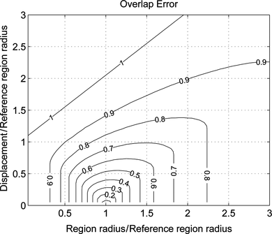
A method integrating all these needs is based on the idea of not establishing an interest point correspondence, but instead a correspondence of regions (Mikolajczyk et al. 2005). This can be justified by the fact that both detector and descriptor work on an image region rather than on image points. The region size of the detector and descriptor windows is proportional to the feature scale. Figure 5 shows successfully matched corresponding regions in AFM and SEM scans detected on an nanocluster sample using the SIFT detector. The region size has been selected to be the circumcircle of the descriptor window. Region correspondence can be defined with the help of the overlap error ϵ _S for two regions, A and B:

The formula is based on the ratio between intersection and union of the regions, and returns an overlap error of zero for identical regions. According to (Mikolajczyk et al. 2005), region correspondence is assumed for overlap errors <50%. In this case, strong descriptors are still able to detect feature correspondence. The overlap error ϵ _S between two regions mapped onto each other as a function of difference in region size (proportional to scale) and location can be seen in Figure 6.

Figure 5 Successfully matched corresponding regions on the nanocluster sample using the SIFT detector. The circle diameter indicates the scale on which the region has been detected.

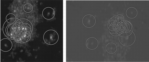
Figure 6 Overlap error between two regions mapped onto each other as a function of difference in region size (proportional to scale) and location. For overlap errors <50%, region correspondence is assumed.

A measure of detector performance is obtained by computing the repeatability score for an AFM and SEM image pair. It is the ratio between the number of feature correspondences and the smaller number of features detected in one of the scans. Only the image areas present in both scans are regarded here. A good detector will reproduce responses in both modalities and therefore yield high repeatability scores. Although the repeatability score provides a realistic view on the expected ability to reproduce results in a different modality, for detector comparison it has a drawback. Using the above definition of ϵ _S , detectors returning large regions are privileged. To avoid this behavior, the detected regions can be rescaled so that each base region (e.g., from the SEM scan) is normalized to the same size and the size ratio between corresponding regions remains untouched.

The descriptor and matching performance can be measured with the help of the recall versus 1-precision plot (Mikolajczyk and Schmid 2005). It measures the ability to detect correct feature correspondences and to reject incorrect matches. Recall and 1-precision are defined as follows:

For a series of varying matching thresholds, the values are plotted on a curve. A good descriptor and matching strategy obtains a high recall rate (detects many of the existing feature correspondences) and a low 1-precision value (returns few incorrect correspondences).

In contrast to the SURF algorithm, the SIFT algorithm allows multiple descriptors for a single feature. During the experiments, a percentage of 15% to 50% of detected SIFT features was found not to be the unique feature point for a location. This has a number of effects on the performance evaluation. In the computation of the detector repeatability, regions which are present multiple times in the dataset obtain a higher weight. Because existing region correspondences as well as missing correspondences are concerned, this effect is minimal. However, in all investigations of detector performance, multiple entries for identical regions have been eliminated. On the other hand, generating multiple descriptors for different orientations is a superior feature of the SIFT matching strategy and should be taken into account in the performance evaluation. Allowing multiple descriptors, as such, brings no preference of the SIFT algorithm in the evaluation of the matching performance, because potentially the number of correspondences and correct and incorrect matches are all increased.

The accuracy of the area-based registration is examined by comparing the obtained transformation with the ground-truth transformation. A direct comparison of the transformation parameters in terms of absolute differences does not provide a good measure of the expected error. For example, an absolute error of 1 in t _x might be acceptable in some applications, but for s _x it is most likely not. Another problem is the dependency between the alignment error and the scan area: in the center of rotation and scale, errors in R and S have no impact. A better performance criterion is described in Capel (2004). The actual transfer error between an estimated transformation , and a ground-truth transformation T (x, y) can be computed from the following:

For symmetry reasons, the displacement error is computed in forward (δ ₁ ) and inverse (δ ₂ ) directions. Over a region of interest Ω the vector field of displacement errors is averaged, which results in the root mean square transfer error e _rms of :

4. EXPERIMENTAL RESULTS

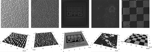
The techniques presented in Section 2 have been tested in five different application scenarios. Image processing has been carried out using the image processing environment of MATLAB (Gonzalez et al. 2004). The image material has been acquired using a Tescan LYRA 3 FEG/XMH (SEM), a Zeiss LEO 1450 (SEM), and a custom-built AFM setup which can be integrated into the vacuum chamber of the SEMs (Mick et al. 2010). All SEM scans are based on the SE detector signal. The AFM scans measure surface topography in intermittent contact mode. All types of samples used can be seen in Figure 7. The goal has been to cover a range of different image contents for obtaining a meaningful performance estimation of the proposed registration procedure. Compact disc (CD) and digital versatile disc (DVD) samples have been prepared for inspection by separating pieces of the data layer. The data layer surface shows structures in blob and dash shape. For obtaining edge-like structures, letters have been milled into a silicon substrate using the focused ion beam (FIB) column of the Tescan LYRA. Gold nanoclusters of varying size have been imaged on a silicon substrate. A test pattern made of gold on a silicon substrate exhibits a lot of square-shaped structure, which is highly ambiguous.

Figure 7 Samples used during experiments, scanned by SEM (upper row) and AFM (lower row): CD surface, DVD surface, FIB-milled pattern, gold nanoclusters, and gold on silicon test pattern (left to right).

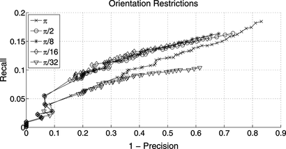
The result of the detector performance analysis is shown in Figure 8 for the DoG (SIFT) and modified DoH (SURF) detectors. On the CD and DVD samples, the SURF detector is slightly superior. For the FIB-milled pattern, nanocluster and gold on silicon pattern, the SIFT detector performs better. On average, the repeatability values are comparable to those reported in Bay et al. (2008) under scale and rotation. For the following task of feature matching, the detector repeatability is sufficiently high in all cases. A set of successfully matched feature pairs for the DVD sample can be seen in Figure 9. Figure 10 studies the effect of restricting differences in the scale ratio during the matching procedure. SIFT-features computed on the DVD sample have been used for this experiment. Although the 1-precision values can be improved by this post-matching step, the recall rate decreases noticably. An improvement of the overall performance is only observed for a moderate restriction of scale ratios by allowing 25% of deviation from the ground-truth scale ratio. On the other hand, introducing restrictions on the allowed difference in orientation leads to a strong gain of performance. Figure 11 shows the recall versus 1-precision plot for a different amount of deviation from the ground-truth difference in angle. The level of π corresponds to the absence of any restrictions. At the very restrict level of π/32, the performance falls below the unrestricted case. It has to be noted that the ground-truth rotation R is accurate in this case. Using a biased estimate of R the performance gain caused by orientation restrictions will be smaller.

Figure 8 Detector performance in terms of repeatability for all samples. A high repeatability means that if a feature is detected in the AFM scan, it is likely to find a corresponding feature in the SEM scan. Feature correspondence is defined by an overlap error <50%. Due to the aspect of multimodality, a lower repeatability is obtained here as compared to monomodal registration (e.g., photograph stitching).

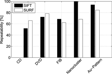
Figure 9 Feature correspondences between an image pair of the DVD sample set. Only correct matches are displayed. The left image shows the AFM scan, and; the right image shows the SEM scan.

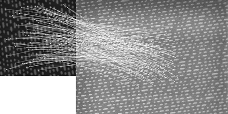
Figure 10 Performance of the scale ratio restriction approach, depicted by the recall 1-precision plot for SIFT features computed on the DVD sample. A moderate restriction allowing 25% of deviation from the ground-truth reproduction scale slightly improves the performance in comparison to the unrestricted case (allowing ∞ deviation). By further increasing the restrictions, the performance decreases because correct matches with imprecisely detected scale are then incorrectly rejected.

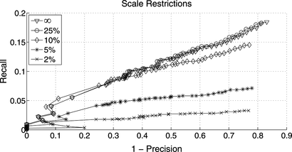
Figure 11 Performance of orientation difference restriction approach, depicted by the recall 1-precision plot for SIFT features computed on the DVD sample. Even low restrictions such as a deviation of π/2 from the ground-truth rotation result in a significant gain in performance. For very high restrictions such as a deviation of π/32, the performance falls below the restriction-free case.

The overall matching performance is compared in Figures 12-16. Experiments have been carried out using regions detected by the SIFT and SURF detectors. Therefore, the number of ground-truth correspondences used to compute the recall rate is different for SIFT and SURF matching. The plot shows that the SIFT algorithm outperforms the SURF algorithm in almost all situations. Generally, the performance is best for the CD, DVD, and nanocluster matching. These are the samples with blob- and dash-shaped structures. The FIB-milled pattern and the gold on silicon test pattern exhibit mostly edge- or corner-like structures and the matching performance is comparably low in both cases. For the FIB-milled pattern, the 1-precision can be improved significantly by using matching restrictions. In contrast, the improvement is moderate for the gold on silicon test pattern sample. In this case, the algorithm performance suffers from the highly ambiguous image structure. No application could be found where the extended SURF descriptor (SURF128) is superior to the regular descriptor (SURF64).

Figure 12 Matching performance for the DVD sample and multiple detector/descriptor combinations, and matching restrictions on scale ratio (S, 25%) and rotation (R, π/16). The SIFT algorithm clearly outperforms the SURF algorithm. The regular-sized SURF descriptor (64) outperforms the extended (128) SURF descriptor.

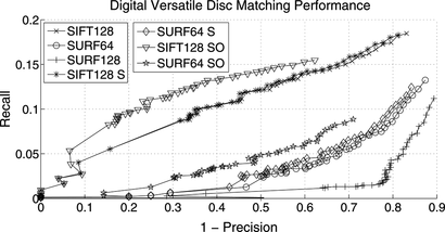
Figure 13 Matching performance for the CD sample and multiple detector/descriptor combinations, and matching restrictions on scale ratio (S, 25%) and rotation (R, π/16).

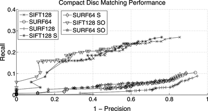
Figure 14 Matching performance for the FIB-milled pattern and multiple detector/descriptor combinations, and matching restrictions on scale ratio (S, 25%) and rotation (R, π/16).

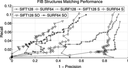
Figure 15 Matching performance for the nanocluster sample and multiple detector/descriptor combinations, and matching restrictions on scale ratio (S, 25%) and rotation (R, π/16).

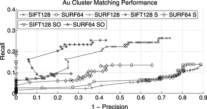
Figure 16 Matching performance for the gold on silicon test pattern and multiple detector/descriptor combinations, and matching restrictions on scale ratio (S, 25%) and rotation (R, π/16). Matching restrictions on SURF features bring moderate gains in performance, but have been left out for clarity reasons.

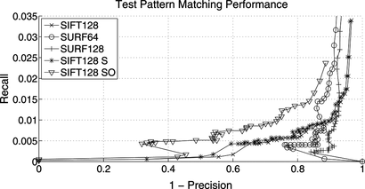
Table 1 shows the execution times measured on an Intel Core i5-750 with 4GB RAM. Only the regular SIFT and SURF algorithms have been evaluated under the aspect of execution time. The values strongly depend on the scene contents and the scan size. On average, the SIFT-based registration takes 3.21 times more computation time. The values have been split up into feature extraction (detection and description), initial matching, and refinement (RANSAC). The computational burden of matching restrictions is negligible and has not been taken into account.

Table 1. Average computation times of the different setups

Setup	SIFT extraction	SIFT matching	SIFT refinement	SURF extraction	SURF matching	SURF refinement
CD	5.33s	0.11s	0.14s	1.81s	0.60s	0.14s
DVD	7.55s	1.07s	0.11s	3.53s	1.05s	0.17s
FIB	22.30s	1.21s	0.44s	2.66s	0.08s	0.49s
Nanocluster	4.84s	0.02s	1.03s	0.69s	0.01s	0.38s
Au-Pattern	8.71s	5.61s	1.08s	1.19s	0.44s	5.30s

SE detector signals are the most commonly used signals in SEM and all scans inspected above have been SE scans. The question arises whether local feature-based registration is also applicable to AFM- and BSE-based SEM scans. For this purpose, the FIB-milled pattern which can be seen in Figure 7 has been imaged additionally in BSE mode. Compared to the corresponding SE scan, all imaging parameters have remained unchanged: field of view, pixel resolution, working distance, and acceleration voltage. In contrast to the SE scan, the BSE scan is weaker in resolving fine structures and the bright fringes are less pronounced. Only the regular SIFT and SURF algorithms have been tested on the BSE scans. In summary, with identical settings much less feature points are detected in the BSE scan in comparison to the SE scan (SIFT:-76%, SURF:-87%). On the other hand, the matching performance of both algorithms is significantly improved in terms of recall and 1-precision. As a result, the final number of correct correspondences remains sufficiently high. However, BSE scans exhibit material contrast and the only material imaged in this example is silicon. In applications with stronger material contrast, a decrease of the algorithm performance must be expected.

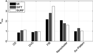
The optimization of the MI criterion has been carried out using the downhill simplex method described by Lagarias et al. (1998) with standard termination criteria. A ground-truth transformation T (x, y) has been computed by linear regression from manually labeled landmark points for all samples. Figure 17 shows the results in terms of e _rms after feature-based registration and after area-based refinement using the MI criterion. The region of interest Ω has been set to a rectangular area centered in the overlap region of the AFM and SEM scan. Application of the area-based registration leads to a moderate reduction of the average error in most applications. However, for the nanocluster sample the average error is increased. This resulted from a slight modification of scale S and rotation R by the optimization procedure. In summary, area-based refinement of the registration result can help to reduce the e _rms error, but does not converge to the ground-truth transformation T (x, y). A reason for this is the anisotropic imaging characteristics of AFM and SEM. They result in the formation of shades and dilatation in dependency of the electron detector position or AFM scanning direction.

Figure 17 Performance results of the area-based registration in terms of e _rms . Values for SIFT and SURF show the remaining error after feature-based registration. MI is the error after area-based refinement of the registration.

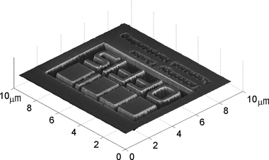
The final result of the system is the fused representation of AFM and SEM scans. Figure 18 shows a three-dimensional view of the DVD surface, textured with the correctly registered SEM scan of the corresponding area. In Figure 19, similar results are shown for the FIB-milled pattern.

Figure 18 Fusion result for the DVD sample. The AFM scan has been rendered as a three-dimensional surface and is textured by the correctly registered SEM scan.

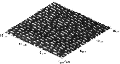
Figure 19 Fusion result for the FIB-milled structure. At the edges of the structure which are facing the SEM's electron detector, a high-intensity SE signal is visible.

5. DISCUSSION AND FUTURE WORK

The proposed procedure has been implemented and tested on a variety of different sample and equipment combinations. In summary, the registration succeeded in all application scenarios. A major benefit of the proposed method over the registration scheme described in Seeger (2004) is the total absence of manual working steps and a minimum number of parameters. In the application scenarios presented here, the feature-based registration faces two imaging modalities with strongly different imaging characteristics and artifacts. These include different intensity levels, morphological changes, shadows, AFM cantilever control-related artifacts, and scanner noise. Under these conditions, generally weaker matching results must be expected as compared to those reported by Mikolajczyk et al. (2005) or Lowe (2004) for natural photography. Nevertheless, the correspondence analysis of pairs of scans is still successful, despite the lower absolute number of correct feature matches.

Both, the SIFT and SURF algorithms have been designed mainly for the registration of natural photographs or video, where the main challenge is to handle changes in illumination or viewpoint and occlusions. It seems that these requirements correspond well with the requirements of AFM and SEM image registration. The aspect of different intensity levels between AFM and SEM is compensated by the normalization of feature vectors. A reduction of the level of sensor noise is integrated in the scale-space approach. Sensor-specific artifacts such as local charging in the SEM scan show the same effect as occlusions in natural photography: features cannot be matches in this local neighborhood, but the performance in the remaining image area is stable.

From the performance evaluation of the feature-based registration, it can be seen that the SIFT algorithm outperforms the SURF algorithm under most aspects. The most-stated advantage of the SURF algorithm is its high speed of computation, which is of minor importance for the task of AFM and SEM image registration. Therefore, the generally preferred algorithm is SIFT. It has been shown that incorporating prior knowledge on the difference in scan orientation or magnification helps to improve the matching performance. In the future, further feature extraction algorithms should be integrated and inspected for their suitability for the registration of AFM and SEM scans.

A limitation of the SIFT and SURF descriptor generation, in the presence of multiple forms of contrast is the computation of the local gradients or wavelet responses, respectively (see Figures 3 and 4). The determination of the dominant feature orientation and local gradient orientations assume a nearly monotonically increasing mapping between AFM and SEM intensity values, and therefore identical gradient orientations in both modalities. Violations of this assumption lead to a total failure of the matching procedure, as the feature orientation and therefore the assignment of local gradients or wavelet responses are incorrect. This limitation can be overcome by adding descriptor copies with inverse orientation to the feature set. However, the negative effect in terms of 1-precision has not been studied yet.

Due to shadowing and morphological differences between the modalities, the SIFT and SURF feature detectors do not reproduce exact feature locations for an image pair. The area-based refinement of the registration result brings a modest improvement but still leaves a significant transfer error. In future investigations, the MI criterion could be compared to alternative criteria. However, all methods considered here work directly on the scan data, and it is possible that the residual error cannot be removed by means of a direct method. Seeger (2004) tries to model the process of AFM and SEM image formation and compensates sensor specific artifacts in order to create a similar image pair for registration. In trade for the potential gain in registration accuracy, a multitude of assumptions have to be made about the imaging process and equipment parameters.

ACKNOWLEDGMENT

This work has been supported in part by the European Community: Project FIBLYS (FIB anaLYSis), CP-TP 214042-2.

REFERENCES

- Bastanlar , Yalin , Alptekin Temizel , and Yasemin Yardimci . 2010 . Improved SIFT matching for image pairs with a scale difference . IET Electronics Letters 46 ( 5 ): 346 – 348 .
- Bay , Herbert , Andreas Ess , Tinne Tuytelaars , and Luc Van Gool . 2008 . Speeded-Up robust features (SURF) . Comput. Vis. Image Underst. 110 ( 3 ): 346 – 359 .
- Beis , Jeffrey S. , and David G. Lowe . 1997 . Shape Indexing Using Approximate Nearest-Neighbour Search in High-Dimensional Spaces. Proc. IEEE Conf. on Computer Vision and Pattern Recognition pp. 1000-1006 .
- Binnig , Gerd , Calvin Forrest Quate , and Christoph Gerber . 1986 . Atomic force microscope . Phys. Rev. Letters 56 ( 9 ): 930 – 933 .
- Capel , David. 2004 . Image mosaicing and super-resolution . London : Springer .
- Fan , Yuan , Qian Chen , Shiva Arun-Kumar , Andrew D. Baczewski , Nick V. Tram , Virginia M. Ayres , Lalita Udpa , and Alan F. Rice . 2006 . Registration of tapping and contact mode atomic force microscopy images. Sixth IEEE Conference on Nanotechnology (IEEE-NANO) 1: 193-196 .
- Fischler , Martin A. , and Robert C. Bolles . 1981 . Random sample consensus: A paradigm for model fitting with applications to image analysis and automated cartography . Commun. ACM 24 ( 6 ): 381 – 395 .
- Gnieser , Dominic , Carl G. Frase , Harald Bosse , and Rainer Tutsch . 2009 . Model-based correction of image distortion in scanning electron microscopy. Proc. of 9th Int. Symp. on Measurement Technology and Intelligent Instruments (ISMTII) 1: 1–147–1–151 .
- Gonzalez , Rafael C. , Richard E. Woods , and Steven L. Eddins . 2004 . Digital image processing using MATLAB . Upper Saddle River , NJ : Prentice Hall .
- Goshtasby , Arthur Ardeshir . 2005 . 2-D and 3-D image registration . Hoboken , NJ : Wiley-Interscience .
- Joachimsthaler , Ingo , Ralf Heiderhoff , and Ludwig Josef Balk . 2003 . A universal scanning-probe-microscope based hybrid system . Measurement Science and Technology 14 ( 1 ): 87 – 96 .
- Lagarias , Jeffrey C. , James A. Reeds , Margaret H. Wright , and Paul E. Wright . 1998 . Convergence properties of the Nelder–Mead simplex method in low dimensions . SIAM J. on Optimization 9 ( 1 ): 112 – 147 .
- Lowe , David G. 2004 . Distinctive image features from scale-invariant keypoints . International Journal of Computer Vision 60 ( 2 ): 91 – 110 .
- Mick , Uwe , Volkmar Eichhorn , Tim Wortmann , Claas Diederichs , and Sergej Fatikow . 2010 . Combined nanorobotic AFM/SEM system as novel toolbox for automated hybrid analysis and manipulation of nanoscale objects. IEEE Int. Conf. on Robotics and Automation (ICRA) pp. 4088–4093 .
- Mikolajczyk , Krystian , and Cordelia Schmid . 2005 . A performance evaluation of local descriptors . Pattern Analysis and Machine Intelligence, IEEE Transactions 27 ( 10 ): 1615 – 1630 .
- Mikolajczyk , Krystian , Tinne Tuytelaars , Cordelia Schmid , Andrew Zisserman , Jiri Matas , Frederik Schaffalitzky , Timor Kadir , and Luc Van Gool . 2005 . A comparison of affine region detectors . International Journal of Computer Vision 65 ( 1/2 ): 43 – 72 .
- Poletti , Giulio , Francesco Orsini , Cristina Lenardi , and Emanuele Barborini . 2003 . A comparative study between AFM and SEM imaging on human scalp hair . Journal of Microscopy 211 ( 3 ): 249 – 255 .
- Reimer , Ludwig. 1998 . Scanning electron microscopy: Physics of image formation and microanalysis . Berlin , DE : Springer .
- Seeger , Adam. 2004 . Surface reconstruction from AFM and SEM images . PhD thesis , University of North Carolina .
- Tarasenko , Olga , Said Nourbakhsh , Spencer P. Kuo , Asya Bakhtina , Pierre Alusta , Dina Kudasheva , Mary Cowman , and Kalle Levon . 2006. Scanning electron and atomic force microscopy to study plasma torch effects on b. cereus spores. IEEE Transactions on Plasma Science 34 (4): 1281–1289.
- Wei , Qufu , Dan Tao , Weidong Gao , and Yubo Huang . 2008 . Scanning electron microscopy and atomic force microscopy of composite nanofibres . Microscopy and Analysis 22 ( 2 ): 11 – 12 .
- Wortmann , Tim. 2009 . Fusion of afm and sem scans. Proc. of Int. Symposium on Optomechatronic Technologies (ISOT) pp. 40–45 .
- Wortmann , Tim. 2010 . Automatic stitching of micrographs using local features. Proc. of Int. Symposium on Optomechatronic Technologies (ISOT). SP-MNM-2 .
- Wortmann , Tim , and Sergej Fatikow . 2009 . Carbon nanotube detection by scanning electron microscopy. Proc. of the Eleventh IAPR Conference on Machine Vision Applications (MVA) pp. 370–373 .
- Zhou , Yi , and Mohammed Omar . 2009 . Pixel-level fusion for infrared and visible acquisitions . Int. Journal of Optomechatronics 3 ( 1 ): 41 – 53 .
- Zhu , Yuan Yuan , Gu Qiao Ding , Jian Ning Ding , and Ning Yi Yuan . 2010 . AFM, SEM and TEM studies on porous anodic alumina . Nanoscale Research Letters 5 ( 4 ): 725 – 734 .