Estimation of design discharge for an ungauged overflow-receiving watershed using one-dimensional hydrodynamic model

Abstract

Design discharge at a location of interest is conventionally determined using flood frequency analysis, precipitation frequency analysis, or national flood frequency equations. However, none of these three methods can be used to estimate the design discharge for ungauged watershed where high flows are from overflows of the watershed's bordering stream(s), such as the Hartsville Coulee watershed located in northwestern Minnesota. The historical high flows in the Hartsville Coulee were from the overflows of the Red River of the North (RRN). The objective of this study was to set up and use a HEC-RAS hydrodynamic model to determine the maximum overflow rate from RRN into the Hartsville Coulee in 1997, when the record flooding occurred. The model was calibrated using the observed daily streamflows at four US Geological Survey (USGS) gauging stations along RRN. The breach, over which the floodwater was spilled into the Hartsville Coulee in 1997, was defined using the topographic data surveyed by US Army Corps of Engineers (USACE). The results indicated that the maximum overflow rate was likely between 250 and 310 m³ s⁻¹. The computed overflow rate in this study was well compatible with the value estimated by USGS based on a field reconnaissance as well as the value estimated by USACE using Manning equation. In generalization, the HEC-RAS hydrodynamic module can be used to estimate design discharges for overflow-receiving drainage areas such as the Hartsville Coulee watershed.

Keywords:

• Flood estimation
• hydraulic modelling
• riverine hydraulics

1 Introduction

Hydraulic engineering structure (e.g. diversion channel) is usually sized in accordance with a required/minimum discharge (USACE 2001a). Conventionally, the discharge was determined as a flow rate that is associated with a recurrence interval (e.g. 50-year), the reciprocal of the probability for the discharge to occur in any given year (Ashkar and Bobee 1988, USACE 2003). However, contemporary projects, such as the proposed Hartsville Coulee (Figure 1) diversion channel in northwestern Minnesota (USACE 1998), may need to be designed to have a conveyance capacity of record peak discharges (USDA 1994). This contemporary design approach is based on a storm event that actually occurred in the history. In contrast, the conventional design approach uses a synthetic storm, which did not occur in the history and may not occur in the future either. Nevertheless, both approaches require a design discharge be determined using a scientifically based method. For a gauged watershed, the record peak discharge is known from available observed flows and the recurrence-interval discharge can be determined using the well-established method of flood frequency analysis (FFA; Griffis and Stedinger 2007). FFA has evolved into a uniform procedure as a result of the research efforts in the decades before the 1980s (e.g. HD 1966, WRC 1977). The detailed description of this procedure can be found in Bulletin 17B (IACWD 1982, Thomas 1985).

Figure 1 Map showing the location of the Hartsville Coulee watershed and the river reaches modelled in this study

For an ungauged watershed receiving no inflow from outside the watershed, the recurrence-interval discharge can be estimated using either the method of precipitation frequency analysis (PFA; USACE 1985, USGS 2002) or the national frequency (NFF) equations (Ries and Crouse 2002). PFA requires that the watershed have long-term (e.g. 10 or more years) precipitation data to generate a reliable intensity duration frequency (IDF) curve (Chow et al. 1988), from which a synthetic storm for the recurrence interval of interest can be determined (USDA-NRCS 2004). The storm is then taken as the input of a hydrologic model (e.g. HEC-1; Ely et al. 1981) to compute the resulting peak discharge (Daniil et al. 2005). This computed discharge is assumed to have a recurrence interval identical to that of the storm (Packman and Kidd 1980, Hotchkiss and McCallum 1995, Levy and McCuen 1999) and is considered as the design discharge though this assumption is not unlikely invalid.

When the IDF curve cannot be developed and/or the hydrologic model cannot be constructed due to insufficient available data and resources, the recurrence-interval discharge may be estimated using the NFF equations as a last resort. These equations, developed and published by the US Geological Survey (USGS; Jennings et al. 1994, Hirsch 2000), use the site-specific parameters (e.g. drainage area and slope length) of a watershed to estimate the peak discharges of various recurrence intervals, including 5-, 10-, 20-, 50-, and 100-year, by assuming that the discharges would be solely generated from the storm run-off within the watershed. That is, the NFF equations are invalid for watersheds that receive inflows from their neighbouring drainage basin(s), which is the case for the Hartsville Coulee watershed (Figure 1) because it could receive breakout flows from the Red River of the North (RRN) during flooding periods.

For an ungauged watershed that receives breakout inflow from outside the watershed, it is impossible to determine recurrence-interval discharges. Alternatively, the record peak discharge can be estimated by analysing the largest breakout flow rate occurred in the history and used as the design discharge. In the Hartsville Coulee watershed, USGS (Bolles and Wang 2003) estimated the record peak discharge by examining the scouring damage to a culvert crossing, while the US Army Corps of Engineers (USACE 2008a) used a steady-state HEC-RAS model to estimate the peak discharge. The USGS method was very empirical and subjective, and greatly simplified the important hydraulic properties of the culvert materials (e.g. erodibility). On the other hand, the HEC-RAS model used by USACE requires the unknown peak discharge as well as the Manning's n values as inputs (USACE 2008b). Because the discharge depends on the Manning's n values (Finnemore and Franzini 2001) and because these values are also unknowns, the model might be unable to give a unique discharge prediction. Practical applications of hydraulic models such as HEC-RAS (e.g. FEMA 1995, PIE 2004) usually take Manning's n as a calibration parameter, i.e. adjust Manning's n to make the model-predicted discharges closely match the corresponding observed values. Although the models have been widely used to compute water surface profiles (e.g. FEMA 1987, 1995) and evaluate the in-stream and off-channel storages (e.g. PIE 2004, USACE 2005), the information on using hydraulic models (in particular, hydrodynamic models) to estimate breakout flows is scarce in literature. The objective of this study was to use a HEC-RAS hydrodynamic model to determine the maximum overflow rate from RRN into the Hartsville Coulee in 1997. In addition to giving a more realistic design discharge for the proposed diversion channel, this study also demonstrates a HEC-RAS application that has not been well documented.

HEC-RAS is one of the most widely used one-dimensional (1D) hydrodynamic models. Its 1D representation scheme of the full depth-averaged equations remains a two-dimensional (2D) treatment and can satisfactorily describe in-channel flows (Tayefi et al. 2007). Previous studies (Horritt and Bates 2002, Chatterjee et al. 2008) indicated that HEC-RAS can be calibrated to have a simulation performance compatible with or better than that of 2D and/or coupled 1D–2D models. The overflow into the Hartsville Coulee in 1997 was fully confined in the channel (USACE 1998). Herein, HEC-RAS was used to achieve the aforementioned objective of this study.

2 Description of HEC-RAS

HEC-RAS is designed to perform 1D hydraulic calculations for a full network of natural and constructed channels (USACE 2008a). It supports steady and unsteady flow water surface profile calculations. The hydraulic calculations for cross-sections, bridges, culverts, and other hydraulic structures that were developed for the steady flow component were incorporated into the unsteady (i.e. hydrodynamic) flow module. The unsteady flow module has the ability to model storage areas and hydraulic connections between storage areas as well as between stream reaches. However, this module was developed primarily for subcritical flow regime calculations. While the details of HEC-RAS (version 4.0.0) can be found in USACE (2008b), brief descriptions of its hydrodynamic component and how lateral weir is modelled are presented hereinafter to provide the background information for audiences to well judge the results of this study.

Assuming a horizontal water surface at each cross-section normal to the direction of flow, i.e. a negligible exchange of momentum between the channel and floodplain, HEC-RAS distributes the discharge according to conveyance and solves a set of 1D differential equations (Horritt and Bates 2002, Chatterjee et al. 2008, USACE 2008b) using the four-point implicit/box scheme (Szymkiewicz 1996, Freitag and Morton 2007, Tayefi et al. 2007). The differential equations are expressed as

where Q is the total flow; Z is the water surface elevation; the subscripts c and f refer to the channel and floodplain, respectively; and φ is the ratio of the channel conveyance to the total conveyance (i.e. the summation of the channel conveyance and floodplain conveyance).

Within HEC-RAS, the steady flow bridge and culvert routines (Bourdarias and Gerbi 2007) are used to compute a family of rating curves for the structure. During the simulation, for a given flow rate and tail water level, a resulting headwater elevation is interpolated from the curves. For a junction, HEC-RAS applies flow continuity to reaches upstream of flow splits and downstream of flow combinations, whereas stage continuity is used for all other reaches. In addition, upstream boundary conditions are required at the upstream end of all reaches that are not connected to other reaches or storage areas, while downstream boundary conditions are required at the downstream end of all reaches which are not connected to other reaches or storage areas. In this study, a single-valued rating curve and/or normal depth from Manning's equation (Finnemore and Franzini 2001) are specified as the downstream boundary condition.

HEC-RAS models a lateral weir structure using minimum two cross-sections: one upstream and another downstream of the structure. The upstream cross-section can either be right at the beginning of the structure, or it can be a short-distance upstream. The downstream cross-section can be right at the downstream end of the structure or it can be a short-distance downstream. Any number of additional cross-sections can be added in the middle of the structure. HEC-RAS assumes linearly varied slopes for the weir sill and the water surface between any two adjacent cross-sections. The overflow is computed using the standard weir equation (USACE 2008b).

3 Materials and methods

3.1 The Hartsville Coulee and its drainage area

The Hartsville Coulee originates in an area about 30 km southeast of the Grand Forks gauging station (USGS 05082500; Figure 1). Its headwater is adjacent to RRN. The coulee menders northwards approximately 35 km and then empties into the Red Lake River (RLR) at approximately 5 km along RLR upstream of the confluence of RLR and RRN. The coulee has an average channel bed slope of 0.002, an average channel width of 20.5 m, and an average channel depth of 1.5 m. The coulee has three culvert crossings (Figure 1) beneath the 10th Street, the Zavoral Road, and the Bygland Road, respectively. The 10th Street crossing is located at 0.8 km upstream of the coulee mouth, while the Zavoral Road and Bygland Road crossings are located at 4.3 and 4.5 km upstream, respectively.

The Hartsville Coulee watershed has a drainage area of about 150 km². The watershed has a very low topographic relief, with an elevation ranging from 242 to 266 m above mean sea level. As a result, the precipitation and temperature within the watershed vary negligibly with topographic elevation. The annual average precipitation is 490 mm, 25% of which is in the form of snowfall (Slack et al. 1993). The annual average daily temperature varies from −35.5°C in winter to 40°C in summer, with a mean of 3.5°C. Streamflows in the Hartsville Coulee are normally generated from spring snowmelt run-off, but the coulee's historical peak discharge was resulted from the 1997 overflow of RRN (LeFever et al. 1999, USACE 2001a). The overflow occurred between 19 and 26 April, when the flood crest in RRN was above the top elevation of the right river bank in the vicinity of the Thompson Bridge crossing (Figures 2 and 3). The crossing is located approximately 34 km along RRN upstream of the Grand Forks gauging station (USGS 05082500). The peak discharge was fully confined within the coulee channel.

Figure 2 The dimensions of Thompson Bridge

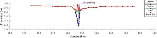
Figure 3 The overtopped RRN right bank section downstream of Thompson Bridge, superimposed by the predicted highest water surface occurred in 1997

As part of the ring dike flood control project in Grand Forks, North Dakota–East Grand Forks, Minnesota (USACE 1998), a diversion channel was proposed to move the existing coulee mouth to a location 4.8 km farther upstream along RLR (USACE 2001a). The landowners to be affected by this proposed diversion requested that the diversion channel be designed using a discharge equivalent to the peak discharge conveyed by the coulee in 1997 (Bolles and Wang 2003). However, the design discharge cannot be determined using either the PFA method or the NFF equations because the peak in the coulee was not generated from the local precipitation run-off. Also, the design discharge cannot be determined using the FFA method because there was no gauging station within the watershed and thus observed data on streamflows are unavailable.

Alternatively, a HEC-RAS hydrodynamic model for the RRN reach between the Halstad gauging station (USGS 05064500) and the Emersion gauging station (USGS 05102500; Figure 1) can be used to estimate the 1997 overflow from RRN into the Hartsville Coulee. The design discharge can be determined as the summation of the estimated peak overflow rate and the local peak flow rate generated from the spring snowmelt run-off by assuming that these two peaks coincided. This assumption tends to give a conservative value for the design discharge, which is preferable for sizing the proposed diversion channel (Bolles and Wang 2003). The local peak flow rate can be predicted using the PFA method. This selected RRN reach includes the river bank section through which the floodwater was spilled into the coulee (Figure 3). In addition, Halstad and Emerson are appropriate as the model boundaries because both stations are sufficiently far away (with a river distance of greater than 95 km) from the overtopped bank section (Kurz et al. 2007).

3.2 Geometric data

The RRN reach between the Halstad and Emerson stations meanders northwards 365 km and includes 19 bridge crossings. The reach was defined using 237 cross-sections positioned by USACE (2001b). The geometric data for these sections were derived from field surveys in reference to the USGS 7.5 min quadrangle maps. In addition, USACE (2001b) provided detailed data on types (e.g. circular or boxed) and dimensions (i.e. opening sizes, pier shapes, and low-chord and high-chord elevations) of the 19 bridge crossings. The data have accuracy sufficient for engineering planning and design purposes, and thus were used in this study.

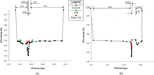
Thompson Bridge has four openings (i.e. three piers; Figure 2). Its minimum low-chord elevation is 253.50 m and maximum high-chord elevation is 256.49 m. In the vicinity downstream of the bridge, the top elevations of the right river bank are overall 0.5 m lower than those of the opposite left river bank. The right river bank section from 75 to 305 m downwards the bridge has an average top elevation of 256.90 m (Figure 3), which was lower than the 1997 flood crest. In this study, this 230 m long section was modelled as a lateral weir using two inclusive RRN cross-sections (USACE 2008a). The weir parameters are described in Section 3.4. The cross-sections for the four RRN gauging stations, namely Halstad, Grand Forks, Drayton (USGS 05092000), and Emerson (Figure 1) are shown in Figures 4 and 5.

Figure 4 The cross-sections at the US Geological Survey (USGS) flow gauging stations at (a) Halstad (USGS 05064500) and (b) Grand Forks (USGS 05082500). The labelled numbers are the calibrated Manning's n values

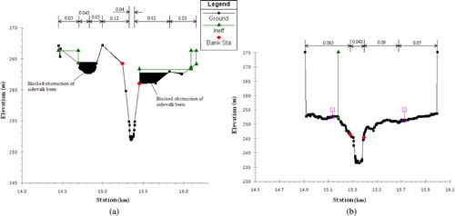
Figure 5 The cross-sections at the USGS flow gauging stations at (a) Drayton (USGS 05092000) and (b) Emerson (USGS 05102500). The labelled numbers are the calibrated Manning's n values

For the modelled reaches of the tributaries except for the one of RLR (Figure 1; Table 1), the cross-sections were extracted from the topographic information presented by the 30 m National Elevation Dataset (NED). NED was developed by merging the highest-resolution, best-quality elevation data available across the USA territory into a seamless raster format (USGS 2001). The extraction was implemented using an ArcView^® GIS extension of Profile Extractor (version 5.5), which can be downloaded at no cost from http://arcscripts.esri.com. The cross-sections for the modelled RLR reach were obtained from USACE (2003). The reaches that are shown in Figure 1 but not listed in Table 1 were not modelled as ‘branch’. Instead, the flows from those reaches were considered as either lateral or point inflows (USACE 2008a; Figure 6). Further, bridge/culvert crossings of the tributaries were not modelled in this study

Figure 6 Schematic of the HEC-RAS model

Table 1 The tributary reaches modelled as branch in this study

State	Tributary^a	Reach below	Length (km)	Number of cross-sections	Predicted 1997 daily peak discharge at the outlet (m^3 s^−1)^b
Minnesota	Marsh River	Shelly	10.73	5	225
	Sandhill River	Climax	3.27	4	128
	RLR^c	Crookston	43.41	53	568
	Snake River	Alvarado	33.21	7	410
	Two Rivers	Lake Bronson	43.92	7	135
North Dakota	Goose River	Hillsboro	17.91	7	218
	Turtle River	Arvilla	67.86	14	64
	Forest River	Minto	31.87	8	84
	Park River	Grafton	27.14	8	209
	Drain20 NR	Glasston	22.68	4	21
	Pembina River	Walhalla	61.40	10	544
^aThe locations of the tributaries are shown in Figure 1.
^bThe peak discharges were predicted using the SWAT models (Kurz et al. 2007). The models can be used to generate flow hydrographs at the outlets of, and at any locations of interest within, the watersheds drained by the tributaries.
^cThe cross-sections were obtained from St Paul District USACE.

3.3 Flow data

USGS has complete records of daily streamflows and stages for the four RRN gauging stations. The data for the period of from 10 April to 10 May 1997, during which the floodwater crested along RRN and was spilled into the Hartsville Coulee, were plotted and are shown in Figures 7–10. The flow hydrograph at Halstad was used to define the upper boundary condition of the HEC-RAS model, whereas the flow hydrographs at the other three stations and the stage hydrographs at all four stations were used to calibrate the model.

Figure 7 The predicted and observed daily streamflows and stages at Halstad

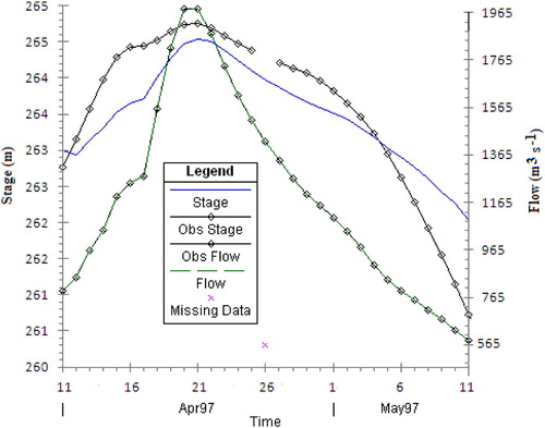
Figure 8 The predicted and observed daily streamflows and stages at Grand Forks

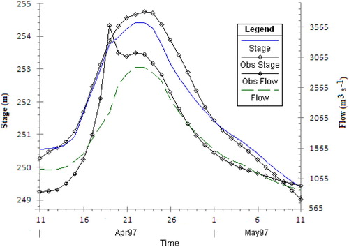
Figure 9 The predicted and observed daily streamflows and stages at Drayton

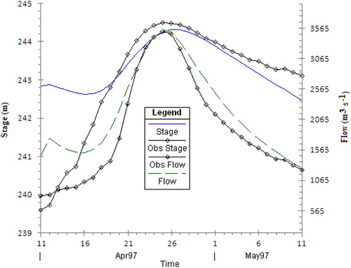
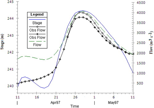
Figure 10 The predicted and observed daily streamflows and stages at Emerson

Some of the tributary stations (e.g. Crookston) shown in Figure 1 have observed data on daily streamflows; the others (e.g. Shelly), however, have either incomplete or no record of streamflows. Further, although a watershed may have a gauging station with a complete record of streamflows, its ungauged area, the drainage area that is not monitored by the station, is generally very large. For example, the 15,110 km² RLR watershed has 1460 km² ungauged area, and totally about 6% of the 250,700 km² drainage area between the Halstad and Emerson stations is not monitored. As a result, the tributary stations provided very limited information that could be used to define the tributary boundary conditions of the HEC-RAS model. Thus, the boundary conditions were defined as the daily streamflows that were simulated using the soil and water assessment tool (SWAT) models of the watersheds drained by the tributaries.

SWAT is a physically based, continuous-time, spatially distributed model that operates on a daily time step and is designed to predict impacts of management practices on water, sediment, and agricultural chemical yields in large ungauged watersheds (Arnold et al. 1998, Arnold and Fohrer 2005). Through a project (Wang et al. 2003a) funded by the US Department of Agriculture Natural Resources Conservation Service, Wang et al. (2003b) set up the SWAT models for the entire RRN basin in the US territory. The models were calibrated and validated using the available daily streamflows for the years from 1978 to 1997. The calibrated models can be used to predict the 1997 flow hydrographs at any locations of interest across the watersheds between the Halstad and Emerson stations. Table 1 shows the SWAT predicted peak discharges at the mouths of the selected tributaries, which are meant for information purposes only. The details about these models and their simulation performances can be found in Kurz et al. (2007).

Further, USACE (2001a) set up an event-based HEC-1 model for the Hartsville Coulee watershed. The basic model input is the equivalent water depth of the accumulated snowpack measured at the Grand Forks International Airport, located at about 2 km west of the watershed. The model predicted that the 1997 snowmelt run-off within the watershed generated a local peak discharge of about 60 m³ s⁻¹. This study presumed that this local peak coincided with the RRN overflow peak. Herein, the design discharge for the proposed diversion channel was simply computed as the summation of these two peak discharge values.

3.4 Model setup

As mentioned above, the observed daily flow hydrograph at Halstad for the study period (i.e. 10 April to 10 May 1997) was used as the upper boundary condition of the HEC-RAS model. On the other hand, the lower boundary condition of the model was specified as normal depths at Emerson for a channel bed slope of 0.000065. This slope was estimated as the ratio of the difference of the channel bed elevations at Emerson and its nearest adjacent upstream cross-section to the river distance between those two locations.

In addition, the SWAT simulated flow hydrographs for the tributaries were specified as either lateral or point inflow boundaries of the model (Figure 6). Further, the river bank section overtopped in 1997 (Figure 3) was modelled as a lateral broad-crested weir with a weir coefficient of C _d = 3.0. The dimensions of the weir were determined based on the data surveyed and provided by courtesy of M.D. Lesher (USACE Hydraulic Engineer, personal email/mail communication, July 2006). The weir was determined to have a side slope (i.e. the ratio of horizontal length to vertical height) of 5, a top width in flow direction of 6.0 m, a breach bottom width of 243.8 m, and a breach bottom elevation of 256.18 ± 0.15 m. The breach was assumed to be a result of overtopping that would start at a water surface elevation of 256.91 m as measured at the weir location in RRN.

The period of 10–13 April was used to stabilize the model parameters (e.g. initial channel storage), whereas the period from 14 April to 10 May was used for model calibration and evaluation. The model was calibrated by manually adjusting the Manning's n values to minimize the differences between the predicted and observed: (1) flow hydrographs at Grand Forks, Drayton, and Emerson, and (2) stage hydrographs at all four RRN stations. The initial Manning's n values were determined in reference to Chow (1959), FEMA (1987, 1995), Mays (2005), and USACE (2005).

3.5 Measure of model performance

The model performance was assessed by comparing the simulated flow and stage hydrographs at the RRN stations with the corresponding observed hydrographs. The comparison was based on visualization plots showing simulated versus observed values. Besides, the comparison was based on the examination of predicted versus observed peaks (magnitudes and timings) and volumes. The volume for a flow hydrograph was computed by integrating the hydrograph throughout the calibration period of from 14 April to 10 May 1997. The volume prediction accuracy was measured using the deviation of volume (D _vj ) statistics, while the peak prediction accuracy was measured using the error function (E _rrj ) statistics (Wang and Melesse 2005).

E _rrj is computed as

where and are the simulated and observed peak discharges, respectively, at station j; and are the timings of the simulated and observed peaks, respectively, at station j; and T _b is the total simulation days, which are 31 for this study.

D _vj is computed as

where Q _simi ^j and Q _obsi ^j are the simulated and observed streamflows, respectively, on the ith time step for station j.

The value of D _vj can range from very small negative to very large positive values, with values close to zero indicating a better simulation and zero indicating an exact prediction of the observed volume. E _rrj can range from 0.0 to +∞, with lower values indicating a better simulation of the observed peak and 0.0 indicating that both the magnitude and timing of the observed peak can be exactly predicted by the model.

3.6 Consideration of streamflow measurement uncertainty for model evaluation

The statistics E _rrj and D _vj assume that the observed data be error free, which is very rarely the case (White et al. 2009). Harmel et al. (2006) examined the approaches currently used to measure streamflow, and found that the uncertainty (i.e. error) in streamflow data can be introduced by potential error sources of (1) individual streamflow measurements to establish the stage-discharge relationship; (2) application of the stage-discharge relationship; (3) continuous stage measurements; and (4) effects of streambed condition on stage measurement. The data uncertainty can be described using ‘probable error range (PER)’, a new statistics developed by Harmel et al. (2006) and discussed in detail by Harmel and Smith (2007). PER is computed as

where n is the number of potential error sources; and E _j is the uncertainty associated with each potential error source j.

A single PER can be applied to all measured data, or a unique value can be calculated for each measured point, depending on the variation of uncertainty throughout the range of measured data. The uncertainty boundaries for each measured value are determined based on estimated PER (Harmel and Smith 2007) as

where UO _i (U) is the upper uncertainty boundary for each measured data point; UO _i (L) is the lower uncertainty boundary for each measured data point; and PER _i is the PER for each measured data point O _i .

In the presence of measurement uncertainty, it is more appropriate to evaluate paired measured and predicted data against the uncertainty boundaries or the probability distribution of measured data than again individual data values. For this purpose, Harmel and Smith (2007) proposed two modifications, modifications 1 and 2, to the difference between each pair of measured and predicted values, such as in Eq. 3 and in Eq. 4. For a range of individual streamflow measurement techniques, channel types, and channel conditions, the absolute value for PER can vary from 6% to 19% (Harmel et al. 2006). Because the specific information on the uncertainty of the daily streamflows observed at the four USGS gauging stations along RRN is unavailable, this study used the above empirical lower bound of 6% to result in tougher model performance requirements (White et al. 2009) while to include some uncertainty to acknowledge that the USGS data used for the model evaluation are not completely error-free. That is, a single PER = ±6% was applied to each observed daily streamflow point for all four stations. Further, because the distribution of uncertainty around each observed streamflow is unknown, this study used Modification 1 to incorporate the measurement uncertainty into Eqs 3 and 4.

Eq. 3 was revised as

Eq. 4 was revised as

Similarly, D _vj (PER) can range from very small negative to very large positive values, with values close to zero indicating a better simulation and zero indicating that all predicted values are within the uncertainty boundary. E _rrj (PER) can range from 0.0 to +∞, with lower values indicating a better simulation of the observed peak and 0.0 indicating that the magnitude of the predicted peak is within the uncertainty boundary and the timing can be perfectly predicted by the model. When including an uncertainty range for observed data, E _rrj (Eq. 3) can decrease in proportion to the size of the uncertainty range, i.e. E _rrj  ≥ E _rrj (PER), and the absolute value for D _vj (Eq. 4) can decrease as well, i.e. . That is, the measure statistics will be improved when the streamflow measurement uncertainty is taken into account for model evaluation.

4 Results and discussion

4.1 Calibrated model

The calibrated Manning's n values for the main channels range from 0.012 to 0.05, while the values for the floodplains vary from 0.03 to 0.2 (Table 2). The lowest value of 0.012 was used for the concrete culvert crossings. For the RRN reach section within which the 1997 floodwater spilled over into the Hartsville Coulee (Figures 3 and 6), Manning's n was adjusted to be 0.035 and 0.115 for the main channel and adjacent floodplain, respectively. The Hartsville Coulee main channel was determined to have a prevalent Manning's n value of 0.028. These calibrated values are very close to those tabulated in the literature (Chow 1959, FEMA 1987, USACE 2003, Mays 2005), and were thus considered to be realistic.

Table 2 Summary of the calibrated Manning's n values

Modelled branch of^a	Main channel n ch	Floodplain n fl
RRN	0.015–0.049	0.05–0.2
Marsh River	0.05	0.12
Sandhill River	0.05	0.12
RLR	0.035–0.05	0.05–0.12
Hartsville Coulee	0.012–0.039	0.036–0.07
Snake River	0.03–0.05	0.03–0.06
Two Rivers	0.05	0.12
Goose River	0.05	0.12
Turtle River	0.05	0.1
Forest River	0.05	0.08–0.15
Park River	0.05	0.12
Drain20 NR	0.05	0.05
^aThese modelled river reaches are shown in Figures 1 and 6.

The model successfully captured the rising and recession limbs of the observed daily flow hydrographs at the RRN stations (Figures 8–10). For Drayton and Emerson, the simulated flow hydrographs closely match the corresponding observed hydrographs. However, the discrepancies before 21 April are relatively larger than those after. One explanation is that the HEC-RAS model could not mimic the mixing flow of ice and water, which was prevalent before 21 April (LeFever et al. 1999). Another explanation is that a longer stabilization period until 21 April may be more reasonable to appropriately initialize the model's parameters (e.g. channel storage). A reasonably long stabilization period is always preferred for continuous-time step simulation models (Wang and Melesse 2005, Wang et al. 2008), including the HEC-RAS hydrodynamic model.

For Grand Forks, the model obviously underestimated the flows for the days of 19 to 25 April. This is because with scarcely available data, the model can inaccurately account for the massive breakout flows that resulted from the overtopping of the RRN dikes in the cities of Grand Forks, North Dakota, and East Grand Forks, Minnesota (Wang et al. 2003b). On the other hand, this may also be because the observed flows for those five days might have very large measurement errors (USACE 2003) as a result of the periodic malfunction of the instruments (C. Anderson, Civil Engineer and President of JOR Engineering, personal oral communication, December 2006).

Accordingly, the simulated stages exhibited similar patterns (Figures 7–10). For Halstad, the model underestimated the average stage by 0.1 m, but the stages before April 21 were underpredicted by up to 0.7 m. Again, this can be partially attributed to that the model parameters might be inappropriately stabilized to represent the river hydraulic conditions until a later date. Nevertheless, given that the prediction errors at Halstad were inevitably propagated to the three downstream stations, it was judged that the model well reproduced the observed stage hydrographs on 21 April and later.

The model well preserved the mass balance of the modelled stream network, as indicated by the small absolute values of D _vi (Table 3) for the RRN stations. The Halstad station had a D _vj value of zero because the observed flow hydrograph at this station was used as the upper boundary condition. The observed volumes at Drayton and Emerson were overpredicted by up to 13.4%, whereas the observed volume at Grand Forks was underestimated by 6.4%. This was expected because the massive breakout flows in the cities of Grand Forks and East Grand Forks bypassed the Grand Forks gauging station (USGS 05082500). These breakout flows were independently estimated (Wang et al. 2003b) and specified in the model as ‘uniform lateral flow’ (USACE 2008a, 2008b) between Grand Forks and Drayton (Figures 1 and 6). Because accurate data on the inundated extent and floodwater depth are not available, the breakout flows might be overestimated. Given this estimation uncertainty, it was judged that the model did a very good job. However, the geometric data on the breached RRN banks do not exist to allow these breakout flows to be modelled using lateral weirs. Also, these breakout flows had no hydraulic connection with Hartsville Coulee (LeFever et al. 1999). That is, none of this breakout floodwater flowed into the coulee.

Table 3 The model performance in predicting peaks and volumes

Station	Peak in 1997						Volume from 14 April to 10 May 1997
	Observed		Predicted		E rr ^a (%)	E rrj (PER)^a (%)	Observed (10^6 m^3)	Predicted (10^6 m^3)	D vj ^b (%)	D vj (PER)^b (%)
	Magnitude (m^3 s^−1)	Timing	Magnitude (m^3 s^−1)	Timing
Halstad^c	1979	April 19	1979	April 19	0.00	0.00	2865	2865	0.00	0.00
Grand Forks	3596	April 18	2900	April 22	23.26	12.90	4457	4171	6.42	3.79
Drayton	3511	April 24	3451	April 24	1.73	0.00	4789	5231	−9.23	−6.36
Emerson^d	4004	April 26	3978	April 27	3.29	3.23	5476	6207	−13.36	−10.65
^a E rrj is error function as defined by Eq. 3, while E rrj (PER) is modified error function as defined by Eq. 3′.
^b D vj is deviation of volume as defined by Eq. 4, while D vj (PER) is modified deviation of volume as defined by Eq. 4′.
^cAs the model upper boundary, the predicted and observed values at this station are identical.
^dThe observed flow hydrograph was provided by Mr A. Warkentin from Manitoba Water Stewardship, Canada. This corrected hydrograph considers the overflows that occurred in 1997 at the west bank of the RRN in the vicinity of Emerson. In contrast, the USGS data did not consider the overflows.

The model well predicted the observed peaks at Drayton (E _rrj  = 1.73%) and Emerson (E _rrj  = 3.29%). The peak discharge at Drayton was underpredicted by 1.7%, while the timing was exactly predicted. In contrast, the peak discharge at Emerson was underestimated by only 0.6%, but the predicted timing was one day later than the observed timing. Further, because the observed peak at Grand Forks might have very large measurement errors, its direct comparison with the predicted peak would make least sense. Nevertheless, the value of E _rrj for this station was computed and is presented in Table 3 for information purposes only.

As expected, the model was judged to have a better prediction performance when the measurement uncertainty in the USGS flow data was taken into account. The predicted peak discharge at Drayton was within the uncertainty boundary and the predicted peak timing coincided with the record (E _rrj (PER) = 0.0). The peaks at Grand Forks and Emerson were better predicted as the values for E _rrj (PER) are smaller than those for E _rrj (Table 3). Similarly, the statistics (D _vj (PER) versus D _vj ) used to measure the model performance in predicting the volumes were improved for all stations.

4.2 Estimated design discharge

The calibrated HEC-RAS model predicted that the overtopping of the RRN right bank section shown in Figure 3 lasted from 20 to 27 April, with about 1.0 × 10⁸ m³ water being spilled into the Hartsville Coulee. Using the average breach bottom elevation of 256.18 m, the model predicted that the daily average maximum overflow rate was 255 m³ s⁻¹ and that this rate probably occurred on 22 April (Figure 11). In addition, a sensitivity analysis with ±0.15 m variations of the breach bottom elevation indicated that the maximum overflow rate could vary between 250 and 300 m³ s⁻¹. Considering the local flow of 60 m³ s⁻¹ generated from the snowmelt run-off within the Hartsville Coulee watershed, the model predicted that the 1997 peak discharge at the coulee mouth reached about 350 m³ s⁻¹ (Figure 12).

Figure 11 The predicted daily overflow hydrograph from the RRN into the Hartsville Coulee

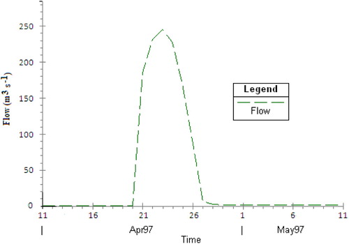
Figure 12 The predicted maximum instantaneous flow profile along the Hartsville Coulee. The zero location is the mouth of the coulee

In May 1997, USGS conducted a field reconnaissance in the vicinity of the Bygland Road crossing (Figure 1; USGS 2002). Through this reconnaissance, USGS defined a 0.20 m head fall through the crossing, and collected data on scour and damage to the pavement and the downstream side of the embankment (Bolles and Wang 2003). Using the combination flow over the road and the Type IV culvert technique (USACE 2008a), USGS estimated a discharge of around 360 m³ s⁻¹. Because the Bygland Road crossing is only 4.5 km above the mouth of the Hartsville Coulee, the USGS estimated discharge can be interpreted as the total maximum flow rate conveyed by the coulee in 1997.

On the other hand, using the aerial photos flown during and after the flooding in conjunction with the USGS 7.5 min topographic quadrangle maps, USACE (2001a) developed typical cross-sections for the highest flood stages along the Hartsville Coulee (Bolles and Wang 2003). By applying Manning equation with empirical roughness coefficients of 0.03 for the main channel and 0.035 for the floodplains, USACE (2001a) determined that the maximum flow rate was around 200 m³ s⁻¹. A subsequent technical review (Wang 2004) revealed that the USACE estimated rate was noticeably low because the roughness coefficients used are unreasonably large. The review indicated that the appropriate Manning's n values be 0.028 for the main channel and 0.039 for the floodplains. These values were verified by a field hydraulic test for a Manitoba channel that has geomorphologic characteristics similar to those of the Hartsville Coulee (M.D. Lesher, USACE Hydraulic Engineer, personal oral communication, December 2002). Therefore, the maximum flow rate of 350 m³ s⁻¹ determined in this study was judged to be compatible with the USGS estimated value as well as the USACE value corrected by using the lower Manning's n values. The proposed diversion channel may be sized to have a conveyance capacity of 350 m³ s⁻¹, as adopted by USACE to design and construct the channel (M.D. Lesher, USACE Hydraulic Engineer, personal email communication, August 2003; S.V. Dobberpuhl, USACE Hydraulic Engineer, personal oral communication, January 2008).

5 Conclusions

This study set up a HEC-RAS hydrodynamic model for the RRN reach between the Halstad and Emerson stations. The observed daily flow hydrograph at Halstad was used as the model upper boundary condition, whereas the model lower boundary condition was defined as normal depths at Emerson for a channel bed slope of 0.000065. The SWAT simulated daily flow hydrographs were used to define the boundary conditions for the tributaries. Further, the 230 m long RRN right bank just downstream of Thompson Bridge, that is, the bank section through which the 1997 floodwater spilled from RRN into the Hartsville Coulee, was modelled as a lateral weir.

The model was calibrated using the observed daily flows at Grand Forks, Drayton, and Emerson, and using the observed daily stages at these three stations as well as at Halstad. The calibration results indicated that the model well reproduced the observed hydrographs, volumes (D _vj  = 6.42% for Grand Forks and −13.4% < D _vj  < 0 for the other three stations), and peaks (E _rrj  = 23.26% for Grand Forks and 0 < E _rrj  < 3.3% for the other three stations). When the measurement uncertainty in the USGS flow data was taken into account, the model was judged to have a better prediction performance, as indicated by the improved statistics D _vj (PER) and E _rrj (PER). The calibrated model predicted that in 1997, about 1.0 × 10⁸ m³ floodwater was spilled from RRN into the Hartsville Coulee, with a maximum overflow rate of 250–300 m³ s⁻¹. Considering the local flow rate of 60 m³ s⁻¹ that was generated from the precipitation run-off within the Hartsville Coulee watershed, the peak discharge conveyed by the coulee in 1997 was likely to be 310–360 m³ s⁻¹. A value within this range can be used as the design discharge for the proposed Hartsville diversion channel. A logical generalization of this study is that the HEC-RAS hydrodynamic module can be used to estimate design discharges for streams that drain overflow-receiving watersheds.

References

- Arnold , J. G. and Fohrer , N. 2005 . SWAT2000: current capabilities and research opportunities in applied watershed modelling . Hydrological Processes , 19 ( 3 ) : 563 – 572 .
- Arnold , J. G. 1998 . Large-area hydrologic modeling and assessment: Part I. Model development . Journal of the American Water Resources Association , 34 ( 1 ) : 73 – 89 .
- Ashkar , F. and Bobee , B. B. 1988 . Confidence intervals for flood events under a Person 3 or log Person 3 distribution . Water Resources Research , 24 ( 3 ) : 639 – 650 .
- Bolles , B. A. and Wang , X. 2003 . Review of the US Army Corps of Engineers' hydraulic study of the Hartsville Coulee diversion, Polk County, Minnesota , 15 Huntsville Township, Minnesota : Final Report for Township Board members .
- Bourdarias , C. and Gerbi , S. 2007 . A finite volume scheme for a model coupling free surface and pressurised flows in pipes . Journal of Computational and Applied Mathematics , 209 : 109 – 131 .
- Chatterjee , C. , Förster , S. and Bronstert , A. 2008 . Comparison of hydrodynamic models of different complexities to model floods with emergency storage areas . Hydrological Processes , 22 : 4695 – 4709 .
- Chow , V. T. 1959 . Open-channel hydraulics , New York : McGraw-Hill .
- Chow , V. T. , Maidment , D. R. and Mays , L. W. 1988 . Applied hydrology , New York : McGraw-Hill .
- Daniil , E. I. , Michas , S. N. and Lazaridis , L. S. 2005 . Hydrologic modeling for the determination of design discharges in ungauged basins . Global NEST Journal , 7 ( 3 ) : 296 – 305 .
- Ely , P. B. , Goldman , D. M. and Feldman , A. D. 1981 . The HEC-1 flood analysis model , 263 – 270 . Reston, Virginia : ASCE, Proc., Water Forum '81 .
- FEMA (Federal Emergency Management Agency) . 1987 . Township of Normanna Cass County, ND. Effective: September 30, 1987 , Washington, DC : Federal Emergency Management Agency, Flood Insurance Rate Map .
- FEMA (Federal Emergency Management Agency) . 1995 . Township of Stanley Cass County, ND. Revised: February 2, 1995 , Washington, DC : Federal Emergency Management Agency, Flood Insurance Rate Map .
- Finnemore , E. J. and Franzini , J. B. 2001 . Fluid mechanics with engineering applications , 10 , New York : McGraw Hill .
- Freitag , M. A. and Morton , K. W. 2007 . The Preissmann box scheme and its modification for transcritical flows . The International Journal for Numerical Methods in Engineering , 70 : 791 – 811 .
- Griffis , V. W. and Stedinger , J. R. 2007 . Evolution of flood frequency analysis with Bulletin 17 . The Journal of Hydrologic Engineering , 12 ( 3 ) : 283 – 297 .
- Harmel , R. D. 2006 . Cumulative uncertainty in measured streamflow and water quality data for small watersheds . Transactions of the ASABE , 49 ( 3 ) : 689 – 701 .
- Harmel , R. D. and Smith , P. K. 2007 . Consideration of measurement uncertainty in the evaluation of goodness-of-fit in hydrologic and water quality modeling . Journal of Hydrology , 337 : 326 – 336 .
- HD (House Document No. 465) . 1966 . A unified national program for managing flood losses , Washington, DC : US Government Printing Office . 89th Congress (2nd Session)
- Hirsch , R. M. 2000 . Vision for the national geospatial framework for surface water . Available from: http://www.crwr.utexas.edu/giswr/events/122000nhda/11/ppt/hirsch.ppt [Accessed 26 November 2009]
- Horritt , M. S. and Bates , P. D. 2002 . Evaluation of 1D and 2D numerical models for predicting river flood inundation . Journal of Hydrology , 268 : 87 – 99 .
- Hotchkiss , R. H. and McCallum , B. E. 1995 . Peak discharge for small agricultural watersheds . Journal of Hydraulic Engineering , 121 ( 1 ) : 36 – 48 .
- IACWD (Interagency Committee on Water Data) . 1982 . Guideline for determining flood flow frequency , Washington, DC : Hydrology Subcommittee, Bulletin No. 17B (revised and corrected .
- Jennings , M. E. , Thomas , W. O. Jr. and Riggs , H. C. 1994 . Nationwide summary of US Geological Survey regional regression equations for estimating magnitude and frequency of floods for ungaged sites , 196 Washington, DC : US Geological Survey, Water-Resources Investigations Report 94–4002 .
- Kurz , B. A. 2007 . An evaluation of basinwide distributed storage in the Red River Basin: the Waffle concept , Bismarck, North Dakota : Final Report for the US Department of Agriculture Natural Resources Conservation Service .
- LeFever , J. A. , Bluemle , J. P. and Waldkirch , R. P. 1999 . Flooding in the Grand Forks – East Grand Forks – North Dakota and Minnesota Area , 63 Bismarck, North Dakota : North Dakota Geological Survey . Educational Series No. 25
- Levy , B. and McCuen , R. 1999 . Assessment of storm duration for hydrologic design . The Journal of Hydrologic Engineering , 4 ( 3 ) : 209 – 213 .
- Mays , L. W. 2005 . Water resources engineering , New York : Wiley .
- Packman , J. C. and Kidd , C. H.R. 1980 . A logical approach to the design storm concept . Water Resources Research , 16 ( 6 ) : 994 – 1000 .
- PIE (Pacific International Engineering PLLC) . 2004 . Draft hydraulic study of Maple River: Maple River and overflow area flood insurance study in Cass County, North Dakota , Denver, CO : FEMA Region VIII, Flood Insurance Study Restudy .
- Ries , K. G. III and Crouse , M. Y. 2002 . The national flood frequency program, version 3: a computer program for estimating magnitude and frequency of floods for ungaged sites , Washington, DC : US Geological Survey, Water-Resources Investigations Report 02-4168U .
- Slack , J. R. , Lumb , A. M. and Landwhr , J. M. 1993 . HCDN: Streamflow data set, 1874–1988 , Reston, VA : US Geological Survey, Water-Resources Investigation Report 93–4076 .
- Szymkiewicz , R. 1996 . Numerical stability of implicit four-point scheme applied to inverse linear flow routing . Journal of Hydrology , 176 : 13 – 23 .
- Tayefi , V. 2007 . A comparison of one- and two-dimensional approaches to modeling flood inundation over complex upland floodplains . Hydrological Processes , 21 : 3190 – 3202 .
- Thomas , W. O. Jr. 1985 . A uniform technique for flood frequency analysis . Journal of Water Resources Planning and Management , 111 ( 3 ) : 321 – 337 .
- USACE (US Army Corps of Engineers) . 1985 . Red River of the North Walsh and Pembina Counties, North Dakota, farmstead flood protection , St. Paul, MN : St. Paul District of US Army Corps of Engineers, Feasibility Report (Supporting Documentation) .
- USACE (US Army Corps of Engineers) . 1998 . General reevaluation report and environmental impact statement: East Grand Forks, Minnesota and Grand Forks, North Dakota , 103 St. Paul, MN : St. Paul District of US Army Corps of Engineers, Final Report of Local Flood Reduction Project Red River of the North .
- USACE (US Army Corps of Engineers) . 2001a . East Grand Forks, Minnesota, 1997 Hartsville Coulee breakout flow , St. Paul, MN : St. Paul District of US Army Corps of Engineers, Memorandum of the US Army Corps of Engineers .
- USACE (US Army Corps of Engineers) . 2001b . Hydrologic analysis: the Red River of the North main stem Wahpeton-Breckenridge to Emerson, Manitoba , St. Paul, MN : St. Paul District of US Army Corps of Engineers, Final Hydrology Report of US Army Corps of Engineers .
- USACE (US Army Corps of Engineers) . 2003 . Regional Red River flood assessment report: Wahpeton, North Dakota-Breckenridge, Minnesota, to Emerson, Manitoba , St. Paul, MN : St. Paul District of US Army Corps of Engineers, Final Report of US Army Corps of Engineers .
- USACE (US Army Corps of Engineers) . 2005 . Hydrology and hydraulics analysis: Fargo-Moorhead upstream feasibility study (phase I) , St. Paul, MN : St. Paul District of US Army Corps of Engineers, Final Report .
- USACE (US Army Corps of Engineers) . 2008a . HEC-RAS river analysis system user's manual , Davis, CA : Hydrologic Engineering Center .
- USACE (US Army Corps of Engineers) . 2008b . HEC-RAS river analysis system hydraulic reference manual , Davis, CA : Hydrologic Engineering Center .
- USDA (US Department of Agriculture) . 1994 . Planning and design manual for the control of erosion, sediment, and stormwater , 1 , Washington, DC : Natural Resources Conservation Service (NRCS) Planning and Design Manual .
- USDA-NRCS (US Department of Agriculture Natural Resources Conservation Service) . 2004 . Peak discharge estimation , Washington, DC : Soil Conservation Measures – Design Manual for Queensland, Natural Resources Conservation Service (NRCS) .
- USGS (US Geological Survey) . 2001 . National Elevation Dataset (NED) , Reston, VA : US Geological Survey Open Report .
- USGS (US Geological Survey) . 2002 . June 2002 floods in the Red River of the North Basin in northeastern North Dakota and northwestern Minnesota , Washington, DC : US Geological Survey, Open-File Report 02–278 .
- Wang , X. 2004 . Technical letter to the township board members, Huntsville township, Minnesota Grand Forks, ND: University of North Dakota (UND) Energy & Environmental Research Center (EERC) Technical Communication Document, 3pp
- Wang , X. and Melesse , A. M. 2005 . Evaluation of the SWAT model's snowmelt hydrology in a northwestern Minnesota watershed . Transactions of the ASAE , 48 ( 4 ) : 1359 – 1376 .
- Wang , X. WaffleSM: an innovative integrated watershed management practice , Council Bluffs, IA: Proc., 8th National Watershed Conference
- Wang , X. A coupled hydrologic–hydraulic model for flood reduction analysis in the Red River of the North , Moorhead, MN: Proc., 1st Int. Water Conference
- Wang , X. 2008 . Simulation of an agricultural watershed using an improved curve number method in SWAT . Transactions of the ASAE , 51 ( 4 ) : 1323 – 1339 .
- White , E. D. 2009 . Improving daily water yield estimates in the Little River watershed: SWAT adjustments . Transactions of the ASABE , 52 ( 1 ) : 69 – 79 .
- WRC (Water Resources Council) . 1977 . Guidelines for determining flood flow frequency , Washington, DC : Hydrology Committee, Bulletin No. 17A .