swmmr - an R package to interface SWMM

ABSTRACT

The stormwater management model SWMM of the US EPA is widely used to analyse, design or optimise urban drainage systems. To perform advanced analysis and visualisations of model data this technical note introduces the R package swmmr. It contains functions to read and write SWMM files, initiate simulations from the R console and to convert SWMM model files to and from GIS data. Additionally, model data can be transformed to produce high quality visualisations. In accordance with SWMM’s open source policy the package can be obtained through github.com or the Comprehensive R Archive Network (CRAN).

KEYWORDS:

• SWMM
• R
• urban drainage modelling
• model data management

1. Introduction

Modelling urban drainage systems has become essential to develop and assess resilient urban stormwater management strategies. Analysing the impact of different climatic or demographic scenarios on urban water infrastructure or optimising urban drainage networks are only some of the applications. Various software products are available to model urban drainage systems. Amongst others, the stormwater management model SWMM (Rossman 2010) is widely used by researchers and practitioners to simulate dynamic hydrology-hydraulic water quality processes. Its source code is released under public domain specification and online available from the US EPA.¹ Besides the availability of the open source engine of SWMM, a pre-compiled software for Microsoft Windows operating systems is available. The software also provides a graphical user interface (GUI) to design drainage networks and to assign attributes to elements of the system. While the open source software facilitates basic analysis and visualisations of model data, advanced features such as time series data management, parameter uncertainty analysis or extended statistics are reserved to commercialised versions of SWMM, only.

FIGURE 1. Example of ggplot2-based visualisation of simulation results.

Figure 2. Visualisation of SWMM Example1 model structure using the ggplot2 package.

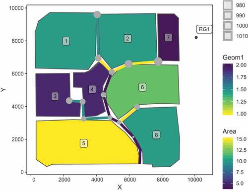
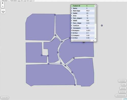
Figure 3. Interactive visualisation of SWMM Example 1 model structure using the mapview package.

In this respect, the free software environment for statistical computing and graphics R (R Core Team 2017) is frequently used by both scientists and engineers. It provides a huge variety of add-on packages which also cover issues related to hydrology in general and urban water modelling more specifically. For example, hydrology specific packages support process-based modelling (e.g. reservoir – Turner and Galelli (2016)), spatial data processing (e.g. Watersheds – Torres-Matallana (2016)), model performance analysis (e.g. hydroGOF – Zambrano-Bigiarini (2017)), or data exploration (e.g. wql – Jassby, Cloern, and Stachalek (2017)). Moreover, packages epanet2toolkit (Arandia and Eck 2018) and epanetReader (Eck 2016) interface R with EPANET² (Rossmann 2010), a widely used water distribution systems model. A more comprehensive list is given in the CRAN Task View ‘Hydrological Data and Modeling’.³

Further packages – not explicitly related to (urban) hydrology – provide functions to perform model parameter optimisation (e.g. DEoptim – Ardia et al. (2016)), visualise data (e.g. dygraphs – Vanderkam et al. (2017); ggplot2 – Wickham (2016)), or manage time series data (e.g. xts – Ryan and Ulrich (2017)). Additionally, with the development of the packages sp (Pebesma and Bivand 2005) and sf (simple features) (Pebesma 2018), R’s spatial data processing capabilities have been significantly advanced. Consequently, as modelling in general involves both pre- and post-processing of different types of data such as spatial or time series data, the availability of these packages enables an efficient model data management and allows various modelling tasks of diverging complexity to be addressed.

To bridge the gap between urban drainage modelling and advanced model analytics, we herein introduce the freely available R package swmmr which provides functions to interface SWMM. Core functions of the package comprise fast reading and writing of SWMM files, conversion between GIS data and the SWMM input file format as well as model data transformation to produce expressive visualisation. This technical note describes design principles of the swmmr package and exemplifies its usage. This includes a demonstration of how to produce high quality figures of model results and model structures enabled by further R packages.

2. What is the package useful for?

The main purpose of the swmmr package is to assist the modeller during the modelling process. Typically, this includes processing and visualisation of measurement and spatial data, which the R ecosystem provides matured packages for. However, its capabilities of interactively creating and modifying spatial data are limited and should not yet be compared to a specialised GIS software, though remarkable progress can be observed (mapview – Appelhans et al. (2018); mapedit – Appelhans and Russell (2017)). Thus, the package is especially useful to modellers who use R for model data management and/or need to perform advanced analysis, visualisation or optimisation tasks of a given model or model results, respectively.

3. Package design and core functions

At its core, the package relies on the tidy data concept (Wickham 2014) which is expressed through a set of harmonised packages sharing common data representation principles (‘tidyverse’ – Wickham (2017)). Although most tasks could have been addressed with base R,⁴ packages from the ‘tidyverse’ tend to simplify both the programming and the data analysis. For example, swmmr uses tibbles (Müller and Wickham 2017) instead of R’s built-in data.frame to represent SWMM sections because tibbles have a convenient print method which only shows the first 10 rows of data, and all the columns that fit on screen (Wickham and Grolemund 2016). This becomes especially useful when dealing with large SWMM data using functions such as read_inp(), read_rpt() and read_lid_rpt() (Table 1) as the console output remains readable in case large data have been printed. Generally, these functions take the path to a corresponding SWMM file (*.inp or *.rpt) and parse its content to a named list of tibbles or a single tibble, respectively. read_inp() creates an object of class inp, whose list element names are identical to the names of SWMM input sections available in lower letters (e.g. options, subcatchments, etc). To print a summary or to quickly visualise the model structure of the inp object, two generic functions summary() and autoplot() for inp objects are implemented. read_rpt() creates a named list of class rpt containing summary sections from the report file of SWMM (e.g. subcatchment_runoff_summary). While both of the aforementioned functions maintain the original SWMM file structure, read_lid_rpt() interprets text files from specific LID elements. A single tibble or index-based time series data as xts object is returned accordingly. The latter option is provided because xts objects, which are introduced with the xts package and build upon R’s built-in matrix data type, efficiently represent time series data and offer index-focused data subsetting methods.

Table 1. Functions for the R environment provided by swmmr.

Name	Inputs	Description
model run
run_swmm()	path to .inp (optional: .rpt and .out file)	Initiate a SWMM run from the R console
reading files
read_inp()	path to .inp file	Reads a SWMM model as list of tibbles (i.e. inp object)
read_out()	path to .out file	Reads SWMM simulation results (time series) as list of xts objects
read_rpt()	path to .rpt file	Reads SWMM simulation results (summary) as list of tibbles
read_lid_rpt()	path to LID report file	Reads a SWMM LID Report File as tibble or xts object
writing files
write_inp()	inp object (optionally modified) and filename	Writes an inp file to disk which can be read and run by SWMM
simple feature conversion
*_to_sf()	inp object	Converts SWMM objects as tibble with simple feature geometries (supported objects are junctions, links, orifices, outfalls, pumps, raingages, storages, subcatchments, weirs)
inp_to_sf()	inp object	Converts an entire inp object as list of tibbles with simple feature geometries
.shp file conversion
inp_to_files()	inp object, model name and directory path	Converts .inp to .shp and .txt files
shp_to_inp()	s. package manual	Converts .shp files as list of tibbles (i.e. inp object)
generic functions
summary()	inp object	Prints a summary of the SWMM model structure
autoplot()	inp object	Produces a default plot of a SWMM model structure using ggplot2

Reading simulation data from the binary .out file is supported by read_out(). Because .out files can become very large, the function design aims for fast data processing and embeds modern C++ code through Rcpp (Eddelbuettel and Francois 2011). Output data per system element and model variable is always represented as an xts object and conveniently stored in a list environment.

The function write_inp() writes an inp object to disk, which addresses cases where an inp object has been modified within R and changes need to be saved back to disk (e.g. model parameter calibration). Thus, it takes an existing inp object and creates a model file on disk which can be read and run by the original SWMM executable. However, a SWMM simulation run can also be initiated from the R console with run_swmm(). It requires the path to an .inp file to be specified and calls the SWMM executable. The function conveniently returns a 3-element list containing paths to the .inp, .rpt and .out file.

Moreover, converting SWMM input sections with spatial reference to sf objects is supported with *_to_sf() functions. Based on the conversion of SWMM input sections to sf objects, an inp object can be converted to the popular .shp format with inp_to_files(). Additionally, .txt files containing simulation settings, storage and pumping curves are returned as well as files containing SWMM time series data. As a counterpart the function shp_to_inp() converts spatial data given in .shp files into an object of class inp. Information on simulation settings, rainfall time series etc. can be given in .txt files to complete the model data. While the conversion to sf objects already enables common spatial analysis of SWMM model data in R, this also allows using the plotting interface of ggplot2 through geom_sf().

4. Example usage

In this work, the basic usage of the package is demonstrated using the model ‘Example1’ which is included in the SWMM software for Microsoft Windows. The model file is usually located at ‘C:/Users/../Documents/EPA SWMM Projects/Examples/Example1.inp’. Alternatively, it is also attached to the package (cf. Listing 1). In addition, the reader is referred to three package vignettes which cover topics beyond the scope of this technical note. For example, instructions on how to auto-calibrate a SWMM model with swmmr or how to convert GIS and SWMM model data with swmmr are given.

4.1. Setup and model execution

To install swmmr from CRAN and to add its namespace to R’s search list, the following commands need to be executed from the R command line (Listing 1). In this example, the model file attached to the package is used and its path is assigned to the variable inp_path. Subsequently, run_swmm() initiates a model run.

if (!require(“swmmr”)) install.packages(“swmmr”)

library(swmmr)

library(tidyverse)

inp_path <- system.file(“extdata”, “Example1.inp”, package = “swmmr”)

swmm_files <- run_swmm(inp = inp_path,

            rpt = tempfile(),

            out = tempfile())

Listing 1 Installation and model execution.

4.2. Analysis of model data

SWMM’s model files (.inp, .rpt and .out) can be accessed from the named list variable swmm_files. Since the results of both the read_inp() and read_rpt() function comprises a list of named tibbles (Listings 2 and 3), elements can be accessed via R’s common extracting mechanism.

inp_object <- read_inp(swmm_files$inp)

summary(inp_object)

Table

#>
#> ** summary of swmm model structure **
#> infiltration	:	horton
#> flow_units	:	cfs
#> flow_routing	:	kinwave
#> start_date	:	01/01/1998
#> end_date	:	01/02/1998
#> raingages	:	1
#> subcatchments	:	8
#> aquifers	:	0
#> snowpacks	:	0
#> junctions	:	13
#> outfalls	:	1
#> dividers	:	0
#> storages	:	0
#> conduits	:	13
#> pumps	:	0
#> orifices	:	0
#> weirs	:	0
#> outlets	:	0
#> controls	:	0
#> pollutants	:	2
#> landuses	:	2
#> lid_controls	:	0
#> treatment	:	0
#> *************************************
inp_object$subcatchments

Table

#>	#	A tibble: 8 x 9
#>		Name	‘ Rain Gage‘	Outlet	Area	Perc_Imperv	Width	Perc_Slope	CurbLen
#>		<chr>	<chr>	<chr>	<int>	<int>	<int>	<dbl>	<int>
#>	1	1	RG1	9	10	50	500	0.01	0
#>	2	2	RG1	10	10	50	500	0.01	0
#>	3	3	RG1	13	5	50	500	0.01	0
#>	4	4	RG1	22	5	50	500	0.01	0
#>	5	5	RG1	15	15	50	500	0.01	0
#>	6	6	RG1	23	12	10	500	0.01	0
#>	7	7	RG1	19	4	10	500	0.01	0
#>	8	8	RG1	18	10	10	500	0.01	0
#>	#	... with 1 more variable: Snowpack <lgl>

Listing 2 Reading and analysing model data.

rpt_object <- read_rpt(swmm_files$rpt)

summary(rpt_object)

Table

#>	Length	Class	Mode
#> analysis_options	2	tbl_df	list
#> runoff_quantity_continuity	3	tbl_df	list
#> runoff_quality_continuity	3	tbl_df	list
#> flow_routing_continuity	3	tbl_df	list
#> quality_routing_continuity	3	tbl_df	list
#> highest_flow_instability_indexes	2	tbl_df	list
#> routing_time_step_summary	2	tbl_df	list
#> subcatchment_runoff_summary	9	tbl_df	list
#> subcatchment_washoff_summary	3	tbl_df	list
#> node_depth_summary	8	tbl_df	list
#> node_inflow_summary	9	tbl_df	list
#> node_flooding_summary	7	tbl_df	list
#> outfall_loading_summary	7	tbl_df	list
#> link_flow_summary	8	tbl_df	list
#> conduit_surcharge_summary	6	tbl_df	list
#> link_pollutant_load_summary	3	tbl_df	list
#> analysis_info	1	tbl_df	list

Listing 3 Reading report of model results.

Time index-based model results from an .out file are imported as given in Listing 4. Here, model variables total rainfall (in/hr or mm/hr, vIndex = 1) and total runoff (in flow units, vIndex = 4) from the system (iType = 3) are read. A general dictionary covering the mapping between variable and index number is included in the package documentation.

sim <- read_out(swmm_files$out, iType = 3, vIndex = c(1,4))

sim$system_variable %>%

do.call(merge, .) %>%

summary

Table

#> Index		total_rainfall	total_runoff
#> Min.:1998-01-01	01:00:00	Min.:0.00000	Min.:0.0000
#> 1st Qu.:1998-01-01	09:45:00	1st Qu.:0.00000	1st Qu.:0.0000
#> Median:1998-01-01	18:30:00	Median:0.00000	Median:0.0000
#> Mean:1998-01-01	18:30:00	Mean:0.07361	Mean:2.1592
#> 3rd Qu.:1998-01-02	03:15:00	3rd Qu.:0.00000	3rd Qu.:0.1033
#> Max.:1998-01-02	12:00:00	Max.:0.80000	Max.:24.2530

Listing 4 Reading and statistical analysis of model results.

4.3. Convert between GIS and SWMM model data

inp_to_files() utilises the conversion functions *_to_sf() for all SWMM sections containing spatial data (Table 1). Sections without spatial information are returned and saved separately. Thus, sub-folders containing .shp, .txt and .dat files are created in a specified directory (Listing 5). Information on supported SWMM sections for both inp_to_files() and shp_to_inp() is given in the package manual.

out_dir <- tempdir()

inp_to_files(x = inp_object, name = “Example1”, path_out = out_dir)

c(“dat”, “shp”, “txt”) %>%

map(list.files(file.path(out_dir,.), pattern = .))

#> [[1]]

#> [1] “Example1_timeseries_TS1.dat”

#>

#> [[2]]

#> [1] “Example1_link.shp” “Example1_outfall.shp” “Example1_point.shp”

#> [4] “Example1_polygon.shp”

#>

#> [[3]]

#> [1] “Example1_options.txt”

Listing 5 Converting SWMM model data into shape files.

Column names of the .shp file attribute table correlate with the original SWMM encoding or its abbreviation to seven characters. shp_to_inp() reads .shp and .txt files and converts them to an inp object (Listing 6). Missing values are completed with default values or can be specified separately. The package vignette provides more information of the conversion details.

converted_inp <- shp_to_inp

(path_options = file.path(out_dir, “txt/Example1_options.txt”),

path_line = file.path(out_dir, “shp/Example1_link.shp”),

path_outfall = file.path(out_dir, “shp/Example1_outfall.shp”),

path_point = file.path(out_dir, “shp/Example1_point.shp”),

path_polygon = file.path(out_dir, “shp/Example1_polygon.shp”),

path_timeseries = file.path(out_dir,”dat/Example1_timeseries_TS1.dat”)

)

summary(converted_inp)

Table

#>
#> ** summary of swmm model structure **
#> infiltration:	horton
#> flow_units:	cfs
#> flow_routing:	kinwave
#> start_date:	01/01/1998
#> end_date:	01/02/1998
#> raingages:	1
#> subcatchments:	8
#> aquifers:	0
#> snowpacks:	0
#> junctions:	13
#> outfalls:	1
#> dividers:	0
#> storages:	0
#> conduits:	13
#> pumps:	0
#> orifices:	0
#> weirs:	0
#> outlets:	0
#> controls:	0
#> pollutants:	2
#> landuses:	2
#> lid_controls:	0
#> treatment:	0
#> *************************************

Listing 6 Converting shape files into SWMM model data.

5. Usage with other R packages

5.1. Visualisation with ggplot2 and mapview

Modelling involves visualisation of spatial and temporal data. With base (R Core Team 2017), lattice (Sarkar 2008) and ggplot2 (Wickham 2016), R currently offers three different plotting systems. Because of ggplot2’s flexibility and declarative way of constructing graphics, a demonstration of how to create expressive and customisable figures of model data is given in Listings 7 and 8.

Listing 7 aims to visualise rainfall and simulated runoff data. Temporal data is read from an .out file, initially merged to one single xts object with two columns (‘total_rainfall’ and ‘total_runoff’) and converted to tibble which can be processed by ggplot2. Both variables are plotted as different geometric objects (geom_col(), geom_line()) and separated into facets. The result is shown in Figure 1.

library(ggplot2)    # ggplot2 ≥ 3.0.0 required

library(broom)      # to convert an xts/zoo object to tibble

sim$system_variable %>%

do.call(merge, .) %>%

tidy(.) %>%

{

 ggplot(mapping = aes(x = index, y = value)) +

  geom_col(data = filter(., series == “total_rainfall”)) +

  geom_line(data = filter(., series == “total_runoff”)) +

  scale_x_datetime(date_breaks = “3 hour”, date_labels = “

  facet_wrap(

    series, ncol = 1, scales = “free_y”, strip.position = “left”,

  labeller = as_labeller(c(

   total_rainfall = “total rainfall (in/hr)”,

   total_runoff = “total runoff (CFS)”

  ))

 ) +

 theme_light() +

 theme(

  strip.placement = “outside”,

  strip.text = element_text(colour = “black”),

  strip.background = element_rect(fill = “white”),

  panel.grid.major = element_blank(),

  panel.grid.minor = element_blank()

 ) +

 labs(

  y = NULL, x = NULL,

  subtitle = paste(range(.$index), collapse = “ - “)

 )

}

Listing 7 Creation of ggplot2-based visualisation of simulation results.

Listing 8 is used to visualise the model structure with subcatchments, links, junctions and raingages. Initially, SWMM objects to be plotted are converted as sf objects. Coordinates for labelling subcatchments and raingages are calculated afterwards. Since ggplot2 provides the geometric object geom_sf()⁵, sf objects are directly passed to ggplot2 and interpreted accordingly. Figure 2 illustrates the result.

# initially, SWMM objects to be plotted are converted as sf objects

# here: subcatchments, links, junctions, raingages

sub_sf <- subcatchments_to_sf(inp_object)

lin_sf <- links_to_sf(inp_object)

jun_sf <- junctions_to_sf(inp_object)

rg_sf <- raingages_to_sf(inp_object)

# calculate coordinates for label position of subcatchments

# here: centroid of subcatchment

coord_subc <- sub_sf %>%

sf::st_centroid() %>%

sf::st_coordinates() %>%

tibble::as_tibble()

# update coordinates to label raingage label

coord_rg <- rg_sf %>%

sf::st_coordinates(.) + 500

tibble::as_tibble()

# add coordinates to tibble containing sf geometries

sub_sf <- dplyr::bind_cols(sub_sf, coord_subc)

rg_sf <- dplyr::bind_cols(rg_sf, coord_rg)

# create the plot

ggplot() +

# subcatchments and label

geom_sf(aes(fill = Area), data = sub_sf) +

geom_label(aes(X, Y, label = Name), sub_sf,

       alpha = 0.5, size = 3) +

# links

geom_sf(aes(colour = Geom1), lin_sf, size = 2) +

# junctions

geom_sf(aes(size = Elevation), jun_sf, colour = “darkgrey”) +

# raingage and label

geom_sf(data = rg_sf, shape = 10) +

geom_label(aes(X, Y, label = Name), rg_sf,

alpha = 0.5, size = 3) +

# change scales and theme

scale_fill_viridis_c() + scale_colour_viridis_c(direction = -1) +

theme_linedraw() +

theme(panel.grid.major = element_line(colour = “white”))

Listing 8 Creation of ggplot2-based visualisation of model structure.

Since sf objects are supported by the mapview package, a SWMM model structure converted to simple feature geometries can also be interactively visualised. Figure 3 shows a screenshot of a browser-based visualisation of the ‘Example1’ model, obtained by executing Listing 9.

library(mapview)

inp_to_sf(inp_object) %>%

mapview()

Listing 9 Creation of mapview-based visualisation of model structure.

5.2. Model calibration using DEoptim

Calibration of model parameters is an essential part within the modelling chain to improve the model quality. During calibration, model parameter values are systematically modified to optimise an objective function, which numerically expresses the difference between observed and simulated data.

Because swmmr provides the functions write_inp() to save an inp object to disk and run_swmm() to potentially run the written model file afterwards, it especially facilitates autocalibration of model parameters. swmmr, however, does not depend on particular optimisation packages. The package vignette ‘How to autocalibrate a SWMM model with swmmr’ exemplifies the application of the DEoptim package (Ardia et al. 2016) for single objective optimisation.

6. Conclusions

A brief introduction of the R package swmmr is given. swmmr interfaces the stormwater management model SWMM with R and bridges the gap between modelling and advanced model analytics. It offers functions to represent SWMM models in R which subsequently can be modified or visualised with modern technologies. Simulation results are efficiently read with help of Rcpp to streamline further time series analysis. This facilitates efficient model calibration and parameter uncertainty analysis. The package is freely available and is especially open to both the SWMM and R community. The authors would like to promote the open source project and welcome any contribution to the package through the project page on GitHub.

Highlights

• An R package to read and write SWMM files is introduced

• SWMM’s .out files are read with high performance

• Functions to convert between GIS and SWMM files are provided

• Modern plotting systems are supported to visualise model data

Software availability

swmmr is available on the Comprehensive R Archive Network (CRAN) at

https://cran.r-project.org/package=swmmr and

GitHub at https://github.com/dleutnant/swmmr

License: GPL-3

System requirements: R (≥3.0.0)

Installation: install.packages(‘swmmr’) or

remotes::install_github(‘dleutnant/swmmr’)

Acknowledgements

This package has been mainly developed in the course of the project STBMOD funded by the German Federal Ministry of Education and Research (BMBF, FKZ 03FH033PX2). Its development was inspired by the work of Peter Steinberg and significantly benefits from the Interface Guide of SWMM (Rossman 2010). In the course of the review of this paper, swmmr evolved from version 0.8.1 to 0.9.0. The latter version also contains contributions by the user community, from which we especially would like to thank Malte Henrichs and Hauke Sonnenberg.

Disclosure statement

No potential conflict of interest was reported by the authors.

Notes

1. https://www.epa.gov/water-research/storm-water-management-model-swmm.

2. https://www.epa.gov/water-research/epanet.

3. https://cran.R-project.org/view=Hydrology.

4. ‘base R’ refers to a set of default packages which R is actually based upon without any additional packages loaded.

5. Note that ggplot2 ≥ 3.0.0 is required.

References

- Appelhans, T., F. Detsch, C. Reudenbach, and S. Woellauer. 2018. Mapview: Interactive Viewing of Spatial Data in R. R package version 2.3.0. https://CRAN.R-project.org/package=mapview
- Appelhans, T., and K. Russell. 2017. Mapedit: Interactive Editing of Spatial Data in R. R package version 0.3.2. https://CRAN.R-project.org/package=mapedit
- Arandia, E., and B. J. Eck. 2018. “An R Package for EPANET Simulations.” Environmental Modelling & Software 107: 59–63. doi:10.1016/j.envsoft.2018.05.016.
- Ardia, D., K. M. Mullen, B. G. Peterson, and J. Ulrich. 2016. DEoptim: Differential Evolution in R. Version 2.2-4. https://CRAN.R-project.org/package=DEoptim
- Eck, B. J. 2016. “An R Package for Reading EPANET Files.” Environmental Modelling & Software 84: 149–154. Accessed 5 July 2017. http://linkinghub.elsevier.com/ retrieve/pii/S1364815216302870
- Eddelbuettel, D., and R. Francois. 2011. “Rcpp: Seamless R and C++ Integration.” Journal of Statistical Software 40 (8): 1–18. doi:10.18637/jss.v040.i08.
- Jassby, A., J. Cloern, and J. Stachalek. 2017. wql: Exploring Water Quality Monitoring Data. R package version 0.4-9. https://CRAN.R-project.org/package=wql
- Müller, K., and H. Wickham. 2017. Tibble: Simple Data Frames. R package version 1.4.1. https://CRAN.R-project.org/package=tibble
- Pebesma, E. 2018. sf: Simple Features for R. R package version 0.6-0. https://CRAN.R-project.org/package=sf
- Pebesma, E. J., and R. S. Bivand. 2005. “Classes and Methods for Spatial Data in R.” R News 5 (2): 9–13. https://CRAN.R-project.org/doc/Rnews/
- R Core Team. 2017. R: A Language and Environment for Statistical Computing. Vienna, Austria: R Foundation for Statistical Computing. https://www.R-project.org/
- Rossman, L. A. 2000. EPANET - User’s Manual Version 2.0. Technical Report. Washington, DC: United States Environmental Protection Agency (US EPA).
- Rossman, L. A. 2010. Storm Water Management Model - User’s Manual Version 5.0. Technical Report. Cincinnati, OH: United States Environmental Protection Agency (US EPA).
- Ryan, J. A., and J. M. Ulrich. 2017. xts: EXtensible Time Series. R package version 0.10-1. https://CRAN.R-project.org/package=xts
- Sarkar, D. 2008. Lattice: Multivariate Data Visualization with R. New York: Springer. ISBN 978-0-387-75968-5. http://lmdvr.r-forge.r-project.org
- Torres-Matallana, J. 2016. Watersheds: Spatial Watershed Aggregation and Spatial Drainage Network Analysis. R package version 1.1. https://CRAN.R-project.org/package=Watersheds
- Turner, S., and S. Galelli. 2016. “Water Supply Sensitivity to Climate Change: An R Package for Implementing Reservoir Storage Analysis in Global and Regional Impact Studies.” Environmental Modelling & Software 76: 13–19. doi:10.1016/j.envsoft.2015.11.007.
- Vanderkam, D., J. J. Allaire, J. Owen, D. Gromer, P. Shevtsov, and B. Thieurmel. 2017. “Dygraphs: Interface to ’Dygraphs’ Interactive Time Series Charting Library.” https://CRAN.R-project.org/package=dygraphs
- Wickham, H. 2014. “Tidy Data.” Journal of Statistical Software 59 (10). Accessed 21 February 2018. http://www.jstatsoft.org/v59/i10/
- Wickham, H. 2016. ggplot2: Elegant Graphics for Data Analysis. Springer-Verlag New York. http://ggplot2.org
- Wickham, H. 2017. Tidyverse: Easily Install and Load the ’Tidyverse’. R package version 1.2.1. https://CRAN.R-project.org/package=tidyverse
- Wickham, H., and G. Grolemund. 2016. R for Data Science: Import, Tidy, Transform, Visualize, and Model Data. 1st ed. Sebastopol, CA: O’Reilly. OCLC: ocn968213225.
- Zambrano-Bigiarini, M. 2017. hydroGOF: Goodness-Of-Fit Functions for Comparison of Simulated and Observed Hydrological Time Series. R package version 0.3-10. https://CRAN.R-project.org/package=hydroGOF