Modelling chlorine wall decay in a full-scale water supply system

ABSTRACT

The use of adequate decay models for simulating chlorine residuals can effectively aid in chlorine management in water supply systems. In this paper, wall decay in a full-scale water supply system is assessed and modelled using the traditional first-order (FO) model and the recent EXPBIO model. The EXPBIO model was successfully implemented in EPANET-MSX for the first time and predicted chlorine residuals with high accuracy. However, in the tested conditions (chlorine residuals ≥0.55 mg/L and small wall decay rates), the FO and the EXPBIO models described chlorine wall decay with similar accuracy. The results suggest that in systems of large diameter pipes and of high disinfectant concentrations, the simpler FO model can be used for the modelling of chlorine residuals without significant loss of accuracy. Further research is needed to identify in which conditions (chlorine levels, wall decay rates) the EXPBIO model performance may exceed that of the FO model.

KEYWORDS:

• Chlorine residuals
• wall decay
• water quality modelling

Introduction

Controlling chlorine residual concentrations is an issue of the utmost importance in the water quality management in drinking water systems. While excessive chlorine residual concentrations may lead to taste and odour related complaints and to the increased formation of disinfection by-products, concentrations below 0.2 mg/L may not be enough for counteracting microbial regrowth (WHO 2017). In addition, chlorine is a very strong disinfectant and reacts with many chemical species in drinking water and, consequently, the residual concentration decreases over time (Deborde and von Gunten 2008). Modelling chlorine decay can be an essential tool for managing water distribution systems, supporting the decision on the injection of disinfectant doses and on the most adequate location of chlorination stations.

Chlorine reacts with dissolved organic and inorganic compounds in water, being this phenomenon known as bulk decay. It reacts as well with some pipe materials (e.g. iron, steel), with biofilm and with loose deposits, which is known as the wall decay (Kiéné, Lu, and Lévi 1998; Gauthier et al. 1999; Clark and Haught 2005). The bulk decay is frequently the predominant chlorine decay mechanism (Kiéné, Lu, and Lévi 1998; Clark and Haught 2005). Chlorine decay in water networks is, thus, often modelled as the sum of the two mechanisms, bulk and wall decay (Minaee et al. 2019a; Munavalli, Mohan Kumar, and Kulkarni 2009). Bulk decay depends on the amount and type of natural organic matter and inorganics in water, hence, water samples should be collected and laboratory decay-tests carried out for assessing decay kinetics, by means of the bottle tests (Powell et al. 2000). First order kinetics is often used for bulk decay modelling given the model simplicity. Single and parallel second order kinetic models, though more complex, are more accurate in predicting chlorine residuals (Fisher, Kastl, and Sathasivan 2011; Monteiro et al. 2017).

Though it may be due to different phenomena (e.g. pipe corrosion, biofilm activity), wall decay is usually modelled as a whole. Two kinetic models are usually used to describe wall decay, namely the zero-order and the first-order models (Vasconcelos et al. 1997). The zero-order kinetic model describes the case in which reaction rate is constant and chlorine is not the limiting reactant. It can be used to model the chlorine decay due to corrosion in cast iron pipes (Kiéné, Lu, and Lévi 1998; Digiano and Zhang 2005). Contrarily, the first-order (FO) kinetic model may represent the chemical reactions in which the decay rate is limited by chlorine concentration at the wall. This concentration depends on the rate of mass transfer from the bulk fluid to the wall and is proportional to the chlorine concentration in water (Rossman, Clark, and Grayman 1994). The mass transfer process can be represented by a film-resistance model, in which chlorine is transported to the wall at a rate proportional to the concentration gradient (Rossman, Clark, and Grayman 1994). For the first order kinetics, the reaction rate at the wall is given by Equation 1 (Rossman 2000).

(1) $\frac{dC}{dt}=-\frac{2k_w{k}_f}{R\left(k_w+k_f\right)}C$(1)

where C is the free chlorine concentration in water (mg/L), k_w is the wall decay coefficient (m/day), k_f is the mass transfer coefficient (m/day) and R is the pipe radius (m). The wall decay coefficient depends on temperature, as any kinetic constant, and has been correlated to pipe age and material. The mass transfer coefficient is often calculated as a function of the molecular diffusivity of the reactive species and of the Sherwood number (Rossman 2000). According to Equation (1), the rate of reaction of chlorine at the pipe wall is always inversely related to the pipe diameter and can be limited by the rate of mass transfer of chlorine to the wall. The FO model has been used to describe chlorine wall decay in pipes of low reactivity materials such as cement lined ductile iron (Digiano and Zhang 2005), PVC and medium-density polyethylene (Hallam et al. 2002) and asbestos cement (Minaee et al. 2019a).

Although chlorine demand for a certain pipe material and diameter can be experimentally determined at the laboratory (Clark et al. 2010; Digiano and Zhang 2005), it may be significantly different from the actual wall decay in a real-life system due to biofilm formation and sediment build-up, which cannot be simulated in laboratory conditions. Hardly any good quality wall demand determination has been carried out in field conditions due to the complexity and the major difficulties in monitoring real systems (Hallam et al. 2002). Grayman et al. (2002) successfully developed a field testing procedure for estimating chlorine wall demand in old, small diameter, unlined cast iron pipes. Fisher, Kastl, and Sathasivan (2017) developed a method for quantifying wall demand in situ, that requires chlorine measurement at each end of the pipes. In full-scale systems with buried pipes, and numerous household connections, it is seldom possible to access many of the nodes in order to take samples or to install monitoring equipment.

For modelling wall decay in full-scale systems, one of the two kinetic models available on EPANET (zero and first-order), is usually chosen and the wall decay coefficient (k_w) calibrated so that the computed chlorine concentrations match the field data (Vasconcelos et al. 1997). All uncertainties and inaccuracies in chlorine decay modelling are incorporated in the wall decay coefficient, including those that arise from the use of inadequate bulk decay models. Chlorine wall decay mechanisms still need to be further investigated and their modelling approach further developed (Grayman 2018).

A new model for wall decay (EXPBIO), combining the effect of biofilm activity moderated by chlorine concentration and mass transport limitation, was developed (Fisher, Kastl, and Sathasivan 2017). The model is based on a previously proposed equation for accounting biofilm formation potential in distribution systems (Hallam et al. 2001) Equation 2.

(2) $B_f=\phi exp\left(nC\right)$(2)

where B_f is the biofilm quantity (pg ATP/cm²), φ is the biofilm constant, n is the chlorine disinfection constant and C is the free chlorine concentration (mg/L). The authors optimised φ and n to 438 and −12.57, respectively, by minimising the sum of the errors between the observed and predicted biofilm potential of Leicester distribution system. Based on Equation 2, and assuming that chlorine decay at the wall is associated to biofilm growth, Fisher, Kastl, and Sathasivan (2017) developed the EXPBIO model Equation 3. Parameters φ and n in Equation 2 were adapted and renamed to A and B, respectively. The model describes chlorine decay as a first order kinetics with respect to both biofilm activity and chlorine concentration at the wall.

(3) $\frac{dC}{dt}=-\frac{4}{D}\frac{Aexp\left(-BC\right)}{1+Aexp\left(-BC\right)/k_m}C$(3)

where D is the pipe diameter (dm) and k_m is a mass transport coefficient (dm/h), A is an amplification factor (dm/h) and B is the rate coefficient (L/mg). The mass transfer coefficient k_m can be computed as a function of the hydraulic conditions in the pipes, as k_f in FO model. Parameters A and B are calibrated so that the model predictions match the observed chlorine concentrations. Neither Hallam et al. (2001) nor Fisher, Kastl, and Sathasivan (2017) provided an explanation for the physical meaning of A and B parameters, which are likely correlated with typical parameters of microbial growth and disinfection kinetics. Again, the calibration of parameters A and B in EXPBIO, as of k_w in FO, accommodates all model uncertainties. The EXPBIO model, not available on EPANET simulator but possible to implement in EPANET-MSX, has not been tested for modelling other full-scale systems besides those used for the model development and validation. The enhanced accuracy of this model compared with the traditional FO modelling has not been demonstrated yet. In this paper, wall decay in a full-scale water transmission system is analysed and modelled by two kinetic models, the FO and the EXPBIO models. The aim is to assess the use of the EXPBIO wall decay model, regarding accuracy, suitability and ease of implementation, compared with the classical FO model. The paper also aims at analysing the model sensitivity to the calibration parameters values.

Methodology

The methodology is based on data collection, sampling and modelling of a full-scale transmission system in Portugal.

Case study

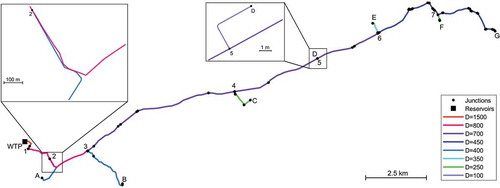
The system comprises a 23 km main trunk that supplies water from Tavira water treatment plant (WTP) to six delivery nodes (A to F in Figure 1), each corresponding to a service storage tank. At node G (Figure 1), water is stored in another tank and rechlorinated, whenever necessary, before following to the downstream part of the transmission system. Pipe diameters range from 1500 to 450 mm in the trunk main, with delivery branches ranging from 100 to 400 mm. Pipes are predominantly made of cement lined ductile iron and the infrastructure has been operating for about 15 years. The system operates at fully turbulent conditions. The characteristics of the pipes (diameter and length) and the system operational conditions (Reynolds number, water age) are presented in detail in Table 1.

Table 1. Characterization of pipes and flow in the case study

Pipe	Diameter (mm)	L (m)	Min Re(-)	Max Re(-)	Average Re(-)	Min water age (h)	Max water age (h)	Average water age (h)
WTP-1	1500	504	390 000	840 000	626 272	1.2	1.3	1.2
1–2	800	1 446	120 000	368 000	255 527	1.8	2.5	2.0
2-A	400	1 054	0	45 000	23 077	4.1	11	5.8
2–3	800	1 575	120 000	352 000	243 834	2.9	4.4	3.4
3-B	400	2 302	76 000	128 000	114 130	4.6	7.0	5.4
3–4	700	6 828	91 000	329 000	213 976	8.3	12	9.7
4-C	250	1 028	0	132 500	381 166	9.2	16	12
4–5	700	3 748	91 000	294 000	200 225	11	14	13
5-D	100	11	8 000	47 000	22 030	12	16	14
5–6	700	2 720	91 000	294 000	197 367	14	18	16
6-E	350	501	0	409 500	135 423	16	22	18
6–7	450	3 265	139 500	364 500	272 183	16	20	18
7-F	250	249	2 500	130 000	45 577	16	26	20
7-G	450	2 967	130 500	301 500	247 234	17	21	19

Figure 1. Case study scheme

A sampling and monitoring programme was carried out over a week in February 2013. Chlorinated water samples were collected at the exit of the WTP for chlorine decay kinetics determination in laboratory. At the WTP, the water had gone through pre-oxidation with ozone, coagulation/flocculation/sedimentation, sand filtration and final disinfection with chlorine. After chlorination, treated water remained in a storage tank for about 3 h before supplying the main trunk. Samples collected for bottle tests were taken immediately downstream the storage tank, i.e. at the beginning of the transmission system, so that the decay observed in laboratory could be representative of the decay observed in the system. Bottle tests were carried out at 10, 15, 20, 25 and 30ºC at the initial concentration of 0.82 mg/L. Grab samples were also taken at each delivery node, from the tanks inlet, for in situ chlorine concentration and temperature measurements. Four samples were collected at each node (except for node F, where only one sample was collected) over a two-day period. All chlorine measurements were carried out with a Pocket Colorimeter II (Hach), which uses the DPD (N,N-diethyl-p-phenylenediamine) method and provides chlorine measurements within 0.05 mg/L accuracy in the low concentration range.

Time series of chlorine concentration at node D, measured by an online analyser (Fischer-Porter), were also collected. Water flow rate data, measured at each delivery node during the monitoring week was also collected and used as demand patterns, specified at the corresponding model nodes.

Water temperature was continuously monitored at the WTP outlet and at nodes B and D. An average water temperature of 13.0ºC was observed throughout the system. During the sampling period, water temperatures varied between 12.9ºC and 14.1ºC, hence, water temperature was considered as almost constant.

Modelling approach

The hydraulic model of the full-scale system was built in EPANET 2.0 (Rossman 2000) based on validated GIS information, measured water flow rates at the delivery nodes and chlorine concentration at the WTP outlet, over one week with one-minute time resolution. The Matlab EPANET toolkit was used (Eliades et al. 2016) integrating the EPANET-MSX features (Shang, Uber, and Rossman 2008). Extended period simulations were carried out (168 h).

For chlorine bulk decay modelling, the two-reactant second order model (2 R model) was chosen (Fisher, Kastl, and Sathasivan 2011) as it has been demonstrated to be adequate for simulating chlorine decay in water distribution systems and has already been successfully used in chlorine decay modelling in the current case study (Monteiro et al. 2014). This model is described by the following equations:

(4) $\frac{d{C}_{Cl}}{dt}=\frac{d{C}_F}{dt}+\frac{d{C}_S}{dt}$(4)

(5) $\frac{d{C}_F}{dt}=-k_F{C}_{Cl}{C}_F$(5)

(6) $\frac{d{C}_S}{dt}=-k_S{C}_{Cl}{C}_C$(6)

where C_Cl is the concentration of free chlorine (mg/L), C_F and C_S are, respectively, the concentrations of fast and slow reducing agents (mg Cl-equiv/L) and k_F and k_S are the fast and slow reaction rate coefficients (L/(mg Cl·day)), respectively. Model parameters were estimated by fitting the 2 R kinetic model to bottle tests results (Figure 2). The decay curve was well described by the 2 R model, though the fast reaction phase was unnoticed, most likely because fast reactants had been oxidized during the pre-oxidation with ozone or in the post-filter storage tank. Determined parameters values were 0.03 and 1.85 mg Cl-equiv/L for fast and slow reducing agents concentration, respectively, and 6.74 and 0.17 L/(mg Cl·day) for fast and slow reaction rate coefficients, respectively.

Figure 2. Bulk decay model (2 R) fitting to bottle test results

Wall decay assessment and modelling

Wall decay was assessed as the difference between the predicted chlorine concentrations by the 2 R bulk decay model and the observed concentrations in the monitored nodes.

Wall decay was modelled by using two kinetic decay models: the FO and the EXPBIO models. The overall chlorine decay was described by combining the 2 R bulk decay model (Equations 4 to 6) with each of the wall decay models, the FO Equation 1 or the EXPBIO Equation 3. Models’ parameters were estimated by minimising the root mean square error (RMSE) between observed and predicted chlorine concentrations at the sampled nodes. Measured chlorine concentrations at the nodes were split into two data sets, one for parameters calibration (13 values) and one for model validation (12 values). Each set included two measured concentrations at each sampled node. The only chlorine measurement at node F was included in the calibration data set.

The particle swarm optimization (PSO) algorithm, available in Brian Birge’s Matlab toolbox (Birge 2003) was used for estimating the optimal parameter values of the wall decay models (A and B in EXPBIO, k_w in FO). The objective function was the minimization of RMSE between measured and predicted chlorine concentrations at the monitored nodes (Minaee et al. 2019b).

PSO is an iterative optimization method based on a population of possible solutions, also known as particles. At each iteration, the objective function is evaluated for every particle, finding the best function value and the best particle location. Based on this information, the particles locations and velocities are upgraded. The iterative process stops when it is reached an optimal state or the maximum number of iterations. The Matlab PSO was set to determine the optimal position of 9 particles, over 2000 iterations, the initial inertia w was set to 0.9 and the acceleration constants c1 and c2 were set to 2.1. The EXPBIO model parameters A and B were initially set to 4 dm/h and 9 L/mg as in Fisher, Kastl, and Sathasivan (2017), while k_w was set with a value of 0.025 m/day (Monteiro et al. 2014). Convergence criterion was set as the lack of improvement of the objective function over 25 consecutive iterations (Brentan and Luvizotto 2014).

The relative quality of FO and EXPBIO models was also assessed by calculating and comparing the corrected Akaike’s Information Criterion (AICc) (Burnham and Anderson 2002).

EXPBIO model parameters sensitivity analysis

The sensitivity analysis of the EXPBIO model parameters was carried out by changing one-factor-at-a-time, either increasing or decreasing each parameter in 10 times its value and assessing the effect on the overall chlorine decay model error. Smaller variations in parameters A and B was also carried out and their effect observed in predicted chlorine concentrations at node D over time.

Results and discussion

Wall decay assessment

Chlorine concentrations predicted by the 2 R bulk decay model at the nodes A, B and C did not differ in more than 0.05 mg/L from measured values; this value is the expected uncertainty associated with in situ free chlorine measurement by the DPD method. Hence, for the set of pipes from the treatment plant to nodes A, B and C, wall decay was not observed. These pipes include diameters of 1500 to 700 mm in the main pipe, 400 mm pipes in the branches to nodes A and B and 250 mm in the pipe branch to node C (Table 1). Free chlorine concentrations in these nodes were in the range of 0.62 to 0.78 mg/L. These results agree with those obtained by Fisher, Kastl, and Sathasivan (2017) that also observed negligible wall decay in large diameter lined pipes (> 500 mm) and chlorine concentrations above 0.5 mg/L. In the current case, the high chlorine concentration in water is likely to have inhibited biofilm activity, even in the smaller diameter pipes.

Measured chlorine concentrations at the nodes further away from the WTP, namely at nodes D, E, F and G, were consistently lower than those predicted by the bulk decay model (Figure 3). Although the difference between measured and modelled chlorine concentrations was small, it was higher than the measurement uncertainty (0.05 mg/L) and it was observed in every sample taken from node D onwards (Figure 4), thus suggesting the occurrence of an additional decay mechanism not described by the bulk decay model. This effect is observed for the first time at node D, located 14 km at downstream from the WTP (Figure 4). The additional chlorine demand is likely due to the wall, as a result of biofilm and sediments accumulation over time.

Figure 3. Correlation plot for the bulk decay model (2 R)

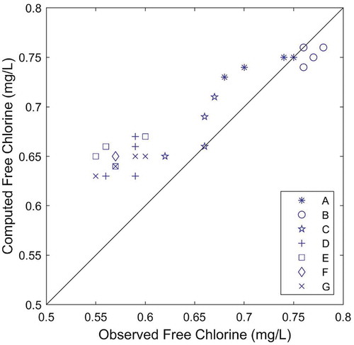
Figure 4. Average chlorine consumption in the system (from the inlet to each monitored node) and percentage of wall decay to overall chlorine demand

Total chlorine consumption in the transmission system, from the inlet to each monitored node, was estimated as the difference between measured chlorine concentrations at the nodes and the corresponding chlorine concentrations at the system inlet, considering the water travelling time. The wall demand was then estimated as the difference between the measured total demand and the bulk predictions by the 2 R model. The results show that the wall demand, observed at the nodes D to G, ranged from 25 to 32% of the overall chlorine decay (Figure 4). Wall decay was observed from node 4 onwards, which includes pipe diameters from 700 to 450 mm in the main trunk and 350 to 100 mm in pipe branches. In this part of the system chlorine concentration was in the range of 0.67 to 0.55 mg/L and the average water residence time varied from 13 to 20 h. Fisher, Kastl, and Sathasivan (2017) did not observe wall demand by biofilm activity at chlorine concentrations higher than 0.5 mg/L. However, biofilms in drinking water systems present very different structural properties and microbial composition, depending on local flow conditions and water quality. In addition, it has been observed that biofilms can develop at the observed chlorine concentrations and higher (Liu et al. 2016). Thus, wall decay in the case study can be due to biofilm activity.

The additional chlorine demand observed at nodes D to G can also result from the inability of the adopted bulk decay model to fully describe chlorine decay in the flowing water. Recent works showed that flow properties (Reynolds number or velocity) can significantly affect the overall chlorine decay, particularly in treated waters of low reactivity (Zhao et al. 2018). As the bulk decay model parameters were obtained from stagnant water in bottles, it is likely that the bulk decay has been underestimated. Also, the observation of an additional chlorine demand only after a certain residence time is also in agreement with Ozdemir and Buyruk (2018) findings, who demonstrated that chlorine bulk decay might change with the travel time of water in a pipe in the absence of wall decay.

In addition, the bulk decay model is based on the assumption of constant reactants concentrations (C_F0 and C_S0) in the water supplying the system. However, during the modelling period, there might have been variations in such concentrations, due to variations in retention time in the upstream storage tank. Thus, the uncertainty in bulk decay estimates can also result from changes in the reactants concentrations that could not have been predicted by the model.

Wall decay modelling

The observed additional chlorine decay was modelled as a wall demand using the traditional FO model and the EXPBIO model. However, it must be highlighted that the case study conditions, namely the large diameter pipes and the high chlorine concentrations (>0.5 mg/L) are different from those in which Fisher, Kastl, and Sathasivan (2017) demonstrated the use of the EXPBIO model.

Optimized first order k_w value was 0.025 m/day, while the estimated EXPBIO model parameters A and B were 1.0 dm/h and 6.2 L/mg, respectively, though other combinations of these parameter were obtained providing similar RMSE. The lack of an available range of expected values for the calibration parameters, published in literature, hampered the search of the optimal set of values.

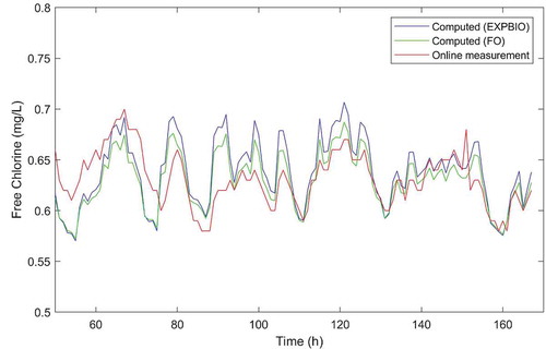
Both the FO and the EXPBIO models, coupled to 2 R bulk decay model, were able to predict chlorine residuals in the system with similar accuracy, as the calculated RMSE for both models were very small (0.02 mg/L). Calculated RMSE values are lower than measuring uncertainty associated with in situ chlorine measurements. Only marginal differences can be found for the results of nodes A and E in the correlation plots (see Figure 5). The accuracy of both models in predicting chlorine over time at node D was also assessed by comparing the model results with online chlorine measurements. In general, both models describe the overall variation trend at this node and both models slightly over predict chlorine concentrations most of the time (Figure 6). The FO model predictions were marginally closer to the measured values than the EXPBIO results.

Figure 5. Correlation plots for the (a) EXPBIO and the (b) FO models

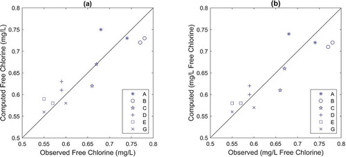
Figure 6. Measured and simulated chlorine concentration over time at node D by FO and EXPBIO models

The Akaike’s Information Criterion (AIC), calculated in its corrected form (AICc) due to the small dataset, was computed for both models in order to determine which of the two models is most likely to be the best one for the current case study. Obtained AICc were −79 and −71 for the FO and the EXPBIO models respectively. Though the model with the absolute lower AICc value is, in general, the better model, the difference between the obtained AICcs is very small. Thus, in the present case, both models describe the dataset in a very similar way.

Overall, these results demonstrate that EXPBIO can be incorporated in EPANET-MSX and that the wall chlorine decay in a full-scale system is satisfactorily predicted by this model. However, the model is more complex than the FO model and its use requires additional programming skills, which can compromise its broader use by the engineers at the water utilities. The model should be further tested in other real-life systems, under different conditions, in order to determine its applicability limits and to identify in which conditions it can predict chlorine residuals better than the FO model.

Sensitivity analysis of the model to parameters’ values

While decreasing A values to 1/10 of its initial value (A = 1.0 dm/h) had a small effect on chlorine decay model accuracy, its increase in 10 times has led to meaningless results (Figure 7(a)). The opposite trend is observed for parameter B (Figure 7(b)), that is, increasing B in 10 times had a small effect on the overall chlorine model accuracy, but decreasing B to 1/10 of its value has led to the prediction of very low chlorine concentrations.

Figure 7. Correlation plots for EXPBIO model when parameters A and B vary by a factor of 10

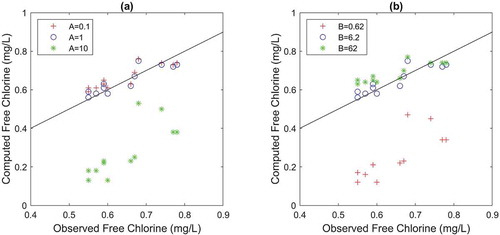
Decreasing A to 0.1 dm/h (Figure 7(a)) and increasing B to 62 L/mg (Figure 7(b)) resulted in an increase in the estimated chlorine concentration at the nodes further away from the WTP, thus diminishing the wall decay mechanism importance and providing similar chlorine values as the 2 R bulk decay model. Conversely, increasing A and decreasing B lead to the prediction of much smaller chlorine concentrations than observed, that is, to an increase in wall effect.

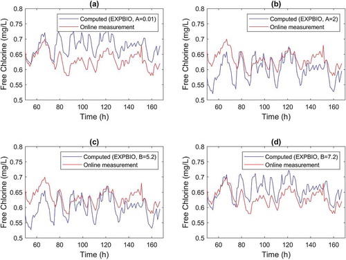
The opposite effect of A and B in model predictions is also observed in the time series for node D when A and B vary by one unit (Figure 8). Parameter A increase from 1 to 2 dm/h resulted in a higher amplitude of predicted chlorine residuals (Figure 8(b)) than that observed when A was reduced to 0.01 dm/h (Figure 8(a)). The opposite trend is observed for B in Figures 8(c,d). Overall, variations in parameter A by one unit resulted in RMSE increase to 0.06 mg/L, while similar variations in B had a smaller increase in the model RMSE, to about 0.04 mg/L (B= 7.2 L/mg) and to 0.05 mg/L (B= 5.2 L/mg).

Figure 8. EXPBIO model predictions for node D by (a) decreasing A to 0.01 dm/h, (b) increasing A to 2 dm/h, (c) decreasing B to 5.2 L/mg and (d) increasing B to 7.2 L/mg

Conclusions

In this paper, chlorine wall decay was assessed and modelled in a full-scale water transmission system.

Wall decay was not observed in the pipes closer to the WTP, which include main pipes of 1500 to 700 mm and smaller pipe branches of 400 and 250 mm. Water age in such pipes was lower than 12 h and chlorine concentrations were in the range of 0.62–0.78 mg/l.

An additional chlorine demand, not described by the bulk decay model alone, was consistently observed in the pipes further away from the WTP. This additional demand accounted for c.a. 30% of the overall decay and was observed in pipes of 700 to 100 mm and at chlorine concentration in the range of 0.67 to 0.55 mg/L. This additional chlorine demand was modelled as wall decay.

The EXPBIO model was successfully implemented in EPANET-MSX, it was tested in the full-scale system modelling and its accuracy in describing chlorine decay was compared with that of the FO model. The results show similar accuracy in predicting chlorine residuals in the case study using the two wall decay models. However, due to a high range of chlorine concentration in the case study (>0.5 mg/L) only small wall decay rates were observed and predicted by the two models, which makes it difficult to assess differences between the two models. In order to fully assess the EXPBIO model capabilities, the model should be further tested in other full-scale water supply systems under different conditions (pipe diameters, chlorine concentration, water age), in order to determine its applicability limits and to identify in which conditions EXPBIO results significantly differ from those predicted by the FO model.

The sensitivity analysis showed that parameters A and B have opposite effects in the model results and that the accuracy of the model is more sensitive to parameter A changes than to parameter B variations. Further studies are needed to better understand the relation between the model parameters and the system characteristics (chlorine concentration, biofilm thickness, pipe material, etc).

Disclosure statement

No potential conflict of interest was reported by the author(s).

Additional information

Funding

The authors acknowledge Fundação para a Ciência e a Tecnologia (PT) for funding the research project IMIST [PTDC/ECI-EGC/32102/2017].

References

- Birge, B. 2003. “PSOt - a Particle Swarm Optimization Toolbox for Use with Matlab” In Proceedings of the 2003 IEEE Swarm Intelligence Symposium 182–186. doi: 10.1109/SIS.2003.1202265.
- Brentan, B., and E. Luvizotto Jr. 2014. “Refining PSO Applied to Electric Energy Cost Reduction in Water Pumping.” Water Research and Management 4 (2): 19–30.
- Burnham, K., and D. R. Anderson. 2002. Model Selection and Multimodel Inference: A Practical Information-Theoretic Approach. 2nd ed. New York: Springer-Verlag.
- Clark, R. M., and R. C. Haught. 2005. “Characterizing Pipe Wall Demand: Implications for Water Quality Modeling.” Journal of Water Resources Planning and Management 131 (3): 208–217. doi:10.1061/(ASCE)0733-9496(2005)131:3(208).
- Clark, R. M., Y. J. Yang, C. A. Impellitteri, R. C. Haught, D. A. Schupp, S. Panguluri, and E. Radha Krishnan. 2010. “Chlorine Fate and Transport in Distribution Systems: Experimental and Modeling Studies.” Journal of the American Water Works Association 102 (5): 144–155. doi:10.1002/j.1551-8833.2010.tb10117.x.
- Deborde, M., and U. von Gunten. 2008. “Reactions of Chlorine with Inorganic and Organic Compounds during Water Treatment – Kinetics and Mechanisms: A Critical Review.” Water Research 42 (1–2): 13–51. doi:10.1016/j.watres.2007.07.025.
- Digiano, F., and W. Zhang. 2005. “Pipe Section Reactor to Evaluate Chlorine—Wall Reaction.” Journal of the American Water Works Association 97 (1): 74–85. doi:10.1002/j.1551-8833.2005.tb10805.x.
- Eliades, D. G., M. Kyriakou, S. Vrachimis, and M. M. Polycarpou. 2016. “Epanet-Matlab Toolkit: An Open-Source Software for Interfacing Epanet with Matlab.” In Proceedings of the 14th Computer and Control for the Water Industry Conference, Amsterdam, The Netherlands, November, 7–9.
- Fisher, I., G. Kastl, and A. Sathasivan. 2011. “Evaluation of Suitable Chlorine Bulk-Decay Models for Water Distribution Systems.” Water Research 45 (16): 4896–4908. doi:10.1016/j.watres.2011.06.032.
- Fisher, I., G. Kastl, and A. Sathasivan. 2017. “New Model of Chlorine-Wall Reaction for Simulating Chlorine Concentration in Drinking Water Distribution Systems.” Water Research 125 (Supplement C): 427–437. doi:10.1016/j.watres.2017.08.066.
- Gauthier, V., B. Gérard, J.-M. Portal, J.-C. Block, and D. Gatel. 1999. “Organic Matter as Loose Deposits in a Drinking Water Distribution System.” Water Research 33 (4): 1014–1026. doi:10.1016/S0043-1354(98)00300-5.
- Grayman, W. M. 2018. “History of Water Quality Modeling in Distribution Systems”. In Proceedings of the 1st International WDSA/CCWI 2018 Joint Conference Kingston, Ontario, Canada, July, 23–25.
- Grayman, W. M., L. A. Rossman, M. A. Gill, Y. Li, and D. E. Guastella. 2002. “Measuring and Modeling Disinfectant Wall Demand in Metallic Pipes”. In EWRI Conference on Water Resources Planning and Management. USA: Roanoke.
- Hallam, N. B., J. R. West, C. F. Forster, and J. Simms. 2001. “”The Potential for Biofilm Growth in Water Distribution Systems”.” Water Research 35 (17): 4063–4071. doi:10.1016/S0043-1354(01)00248-2.
- Hallam, N. B., J. R. West, C. F. Forster, J. C. Powell, and I. Spencer. 2002. “The Decay of Chlorine Associated with the Pipe Wall in Water Distribution Systems.” Water Research 36 (14): 3479–3488. doi:10.1016/S0043-1354(02)00056-8.
- Kiéné, L., W. Lu, and Y. Lévi. 1998. “Relative Importance of the Phenomena Responsible for Chlorine Decay in Drinking Water Distribution Systems.” Water Science and Technology 38 (6): 219–227. doi:10.1016/S0273-1223(98)00583-6.
- Liu, S., C. Gunawan, N. Barraud, S. A. Rice, E. J. Harry, and R. Amal. 2016. “Understanding, Monitoring, and Controlling Biofilm Growth in Drinking Water Distribution Systems.” Environmental Science & Technology 50 (17): 8954–8976. doi:10.1021/acs.est.6b00835.
- Minaee, R. P., M. Afsharnia, A. Moghaddam, A. A. Ebrahimi, M. Askarishahi, and M. Mokhtari. 2019b. “Calibration of Water Quality Model for Distribution Networks Using Genetic Algorithm, Particle Swarm Optimization, and Hybrid Methods.” MethodsX 6: 540–548. doi:10.1016/j.mex.2019.03.008.
- Minaee, R. P., M. Mokhtari, A. Moghaddam, A. A. Ebrahimi, M. Askarishahi, and M. Afsharnia. 2019a. “Wall Decay Coefficient Estimation in a Real-Life Drinking Water Distribution Network.” Water Resources Management 33 (4): 1557–1569. doi:10.1007/s11269-019-02206-x.
- Monteiro, L., D. Figueiredo, S. Dias, R. Freitas, D. Covas, J. Menaia, and S. T. Coelho. 2014. “Modeling of Chlorine Decay in Drinking Water Supply Systems Using Epanet MSX.” Procedia Engineering 70: 1192–1200. doi:10.1016/j.proeng.2014.02.132.
- Monteiro, L., R. Viegas, D. Covas, and J. Menaia. 2017. “Assessment of Current Models Ability to Describe Chlorine Decay and Appraisal of Water Spectroscopic Data as Model Inputs.” Journal of Environmental Engineering 143 (1): 04016071. doi:10.1061/(ASCE)EE.1943-7870.0001149.
- Munavalli, G. R., M. S. Mohan Kumar, and M. A. Kulkarni. 2009. ““Wall Decay of Chlorine in Water Distribution System’.” Journal of Water Supply: Research and Technology—AQUA” 58 (5): 316–326. doi:10.2166/aqua.2009.048.
- Ozdemir, O., and T. Buyruk. 2018. “Effect of Travel Time and Temperature on Chlorine Bulk Decay in Water Supply Pipes.” Journal of Environmental Engineering 144 (3): 04018002. doi:10.1061/(ASCE)EE.1943-7870.0001321.
- Powell, J., J. West, N. Hallam, C. Forster, and J. Simms. 2000. “Performance of Various Kinetic Models for Chlorine Decay.” Journal of Water Resources Planning and Management 126 (1): 13–20. doi:10.1061/(ASCE)0733-9496(2000)126:1(13).
- Rossman, L., R. Clark, and W. Grayman. 1994. “Modeling Chlorine Residuals in Drinking‐Water Distribution Systems.” Journal of Environmental Engineering 120 (4): 803–820. doi:10.1061/(ASCE)0733-9372(1994)120:4(803).
- Rossman, L. A. 2000. EPANET 2 Users Manual. Cincinnati, USA: U. S. Environmental Protection Agency.
- Shang, F., J. G. Uber, and L. A. Rossman. 2008. “Modeling Reaction and Transport of Multiple Species in Water Distribution Systems.” Environmental Science & Technology 42 (3): 808–814. doi:10.1021/es072011z.
- Vasconcelos, J. J., L. A. Rossman, W. M. Grayman, P. F. Boulos, and R. M. Clark. 1997. “Kinetics of Chlorine Decay.” Journal of the American Water Works Association 89 (7): 54–65. doi:10.1002/j.1551-8833.1997.tb08259.x.
- WHO, ed. 2017. Guidelines for Drinking-Water Quality 4th. incorporating the first addendum ed. Geneva, Switzerland.
- Zhao, Y., Y. J. Yang, Y. Shao, J. Neal, and T. Zhang. 2018. “The Dependence of Chlorine Decay and DBP Formation Kinetics on Pipe Flow Properties in Drinking Water Distribution.” Water Research 141: 32–45. doi:10.1016/j.watres.2018.04.048.