Monitoring and characterising the solids loading dynamics to drainage systems via gully pots

ABSTRACT

Runoff (re)mobilises solids and their associated pollutants from streets and transports them via gully pots to the drainage system. As the solids negatively impact the performance of the drainage systems, knowledge on the solids loading in terms of mass and composition is essential. However, monitoring data on the solids loading, in particular, covering all seasons and a number of sites, is scarce. This article presents the results of a monitoring campaign on the solids loading to a drainage system via 52 gully pots over a period of 2 years at a sampling rate of once per 3–4 weeks. The loading shows a maximum during the tree phases ‘leaf growth’ and ‘full capacity’ and is correlated with the rain intensity during these phases. The organic fraction and D₅₀ of the solids are correlated with leaf abscission. The settling velocity of the particles <1800 µm is strongly correlated with their organic fraction.

KEYWORDS:

• Gully pot
• catch basin
• solids
• wash-off
• urban drainage

1 Introduction

1.1. Solids and drainage systems

Urban drainage systems are meant to convey runoff from urban-built areas to prevent urban flooding. Runoff (re)mobilises solids present in these areas and transports them to the drainage system. The solids can accumulate in the drainage system and reduce its hydraulic capacity (e.g. Crabtree 1989; Ashley et al. 1992), which increases the occurrence of flooding, and subsequently the potential exposure of the public to microbial health threats (De Man 2014; Van Bijnen et al. 2018).

Besides, the solids (and the fine solids in particular) carry pollutants (e.g. Sartor and Boyd 1972; Herngren 2005; Deletic and Orr 2005), which should be removed before they are discharged to receiving waterbodies. Combined sewer systems convey runoff to wastewater treatment plants, which reduce the pollutant load and the negative environmental impact. However, during heavy storms, combined sewer overflows (CSOs) may occur, and untreated water is discharged into waterbodies. Separated sewer systems discharge runoff and its suspended solids directly into waterbodies via separate system overflows (SSOs). Both CSOs and SSOs are known to affect the quality of receiving waterbodies (Ellis and Hvitved-Jacobsen 1996).

Given the negative impact of solids on the performance of drainage systems, it is essential to be able to characterise the solids and quantify their loading to the drainage system. To this end, a range of build-up and wash-off models (e.g. Sartor and Boyd 1972; Pitt 1979; Egodawatta, Thomas, and Goonetilleke 2007; Muthusamy et al. 2018) has been proposed. At the same time, monitoring data on the solids loading to drainage systems for model validation, in particular, covering all seasons and a number of sites/a large surface area, is scarce (e.g. Pratt and Adams 1984 monitored 5 drainage inlets for 9–12 months, Ellis and Harrop 1984 monitored 2 drainage inlets during spring and summer; Saget, Chebbo, and Bertrand-Krajewski 1996 monitored 14 sewer basins for 14–17 months, Sansalone et al. 1998 monitored 13 rain events spread over 2 years at 1 drainage inlet, McKenzie and Young 2013 monitored 4 drainage streams for 1 season, Hong et al. 2016 monitored 1 drainage inlet for 6 months; Bonhomme and Petrucci 2017 monitored 1 drainage outlet for 40 days).

1.2. Sources and sinks

The composition of solids present and available for wash-off in urban areas depends on the characteristics of the area and local conditions (Xanthopoulos and Augustin 1992; Rietveld, Clemens, and Langeveld 2020a), and they originate from various sources, such as: traffic, atmosphere, construction activities, weathering of buildings, animal wastes, trash, de-icing materials and vegetation. Many of these sources have a seasonal character, in particular, the effect of vegetation (Pratt and Adams 1984; Ellis and Harrop 1984; Rietveld, Clemens, and Langeveld 2020a) and de-icing (Simperler, Keckeis, and Ertl 2019). Street sweeping is generally regarded as a sink for solids present on streets (Sartor and Boyd 1972; Amato et al. 2010; Hixon and Dymond 2018).

Literature on the effect of these sources and sinks on the total solids loading to drainage systems can be divided into three points of interest: the street surface as the source of solids, the gully pot (also known as catch basin in North America, according to Ellis et al. 2004) as the first recipient part of the drainage system, and within the sewer or drainage system, typically near the SSO.

1.3. Quantification and characterisation

A wide range of sizes has been reported for solids on streets. Bertrand-Krajewski, Briat, and Scrivener (1993) found in their literature review 300< D₅₀ < 400 μm, Lau and Stenstrom (2005) 200< D₅₀ < 350 µm, Droppo et al. (2006) 120< D₅₀ < 660 µm, Zafra, Temprano, and Tejero (2008) 100< D₅₀ < 360 µm, and Gelhardt, Huber, and Welker (2017) 200< D₅₀ < 550 µm. A few researchers reported the density of street solids. Pitt et al. (2005) found 1500 < ρ < 2500 kg/m³ in their literature review and Butler, Thedchanamoorthy, and Payne (1992) found 2100 < ρ < 2510 kg/m³.

Vaze and Chiew (2002) vacuum cleaned and manually brushed street surfaces of 0.5 m². They concluded that the spatial variation of the solids load within a street is high, since the correlation between the solids load on these areas was low. Therefore, large areas need to be monitored to identify the typical solids load and composition on a street.

The composition of solids entering the drainage system is not equal to the composition of solids present on streets, since the transport of solids by runoff causes grading (e.g. Walker and Wong 1999; Vaze and Chiew 2002). Pratt and Adams (1984) found that the magnitude of the solids loading to the drainage system depends on factors related to the transport, rather than on factors related to the availability of solids on the street.

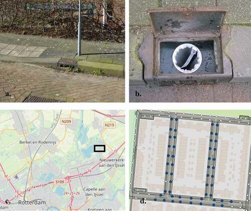
Therefore, monitoring of the solids loading is sometimes performed at the entrance of the drainage system, which is usually a gully pot. The inlet of a gully pot is shown in Figure 1(a). These gully pots have a typical depth of 1 m and a lateral connection with the drainage system. Solids can settle in the volume of the gully pot below this outlet, which is called the sand trap. Grottker (1990) reported a D₅₀ of approximately 400 µm and Pratt and Adams (1984) of 1500 μm for samples from these sand traps. The removal efficiency of solids by the sand trap depends on the solids characteristics, such as the density and size of the solids (e.g. Butler and Karunaratne 1995; Rietveld, Clemens, and Langeveld 2020b). Therefore, the characteristics of the solids transported to the gully pot are not identical to the characteristics of the solids retained in the gully pot.

Figure 1. (a) Gully pot in the monitored streets. (b) Experimental set-up in the gully pot. (c) Map with rectangle indicating the monitoring area. (d) Street map of monitoring area in which the big blue dots indicate the selected gully pots and the small white ones gully pots not selected

To monitor the solids transported to the gully pot, Pratt and Adams (1984) and Ellis and Harrop (1984) installed a stack of sieves in, respectively, five and two gully pots. Pratt and Adams (1984) found a D₅₀ of approximately 680 μm and Ellis and Harrop (1984) a range of 600< D₅₀ < 1000 μm for inflowing solids. Sansalone et al. (1998) redirected the runoff from an area of 300 m² (which is comparable with the surface area connected to 2–3 gully pots) to a storage tank of which samples were taken during 13 rainfall events and reported D₅₀ values between 350 and 800 µm. To be able to represent the solids loading to the drainage system of a catchment, regarding the composition and mass inflow, the number of sampling locations/the monitored surface area needs to be increased significantly.

A more frequently chosen approach to analyse the solids loading to drainage systems is sampling at the outfall or in the sewer pipe. However, collecting representative samples from a drainage pipe is challenging, since solids are both transported as bed and suspended load (Pitt et al. 2017). Boogaard et al. (2014) found 25< D₅₀ < 250 µm and Furumai, Balmer, and Boller (2002) 20< D₅₀ < 80 µm in samples of runoff. Solids collected at the outfall or at least downstream in the drainage pipe, could have been settled and eroded numerous times in the drainage pipe before arrival (e.g. Ashley et al. 2003), such a sample represents an integral over space and time, which smoothens and masks the dynamics of the wash-off processes on the street.

A recent lab study by Naves et al. (2019) demonstrated that wash-off and transport in a drainage system cause grading. An artificial street with two gully pots and a small pipe system was built for replication of the wash-off from the street and the transport in the drainage system. An initial load of sand was placed on the street surface and consecutively artificial rainfall events were created for 5 min. Figure 2 shows the effect of several rainstorm intensities on the particle size distribution (PSD) in different parts of the drainage system.

Figure 2. The particle size distribution after a rainfall event depends not only on the initial street load but also on the rainfall characteristics and the sampling location. The finest particles can be found at the outlet of the system, and larger particles can usually be found in the sand trap of the gully pot. Source: Naves et al. (2019)

Table S1 in the supplementary material shows a brief literature review of sampling locations, measurement methods, and the reported D₅₀ or density.

1.4. Aim of the study

This study aims to provide insight into the drivers and the dynamics of the solids loading, both in mass and composition, to the drainage system over time, by means of a monitoring campaign with a newly designed measurement device, which has been applied to 52 gully pots over a period of 2 years. Sampling in gully pots results in direct information on the dynamics of the solids loading induced by build-up and wash-off processes, while the more common method of sampling in drainage pipes or at outfalls represents an integral over a large space and timescale, which smoothens these dynamics. The results provide information on the variability and predictability of build-up and wash-off related processes.

2. Materials and methods

2.1. Experimental set-up

Pratt and Adams (1984) and Ellis and Harrop (1984) developed a method consisting of a stack of 5 sieves in gully pots to filter the solids out of the runoff, which does not hinder the upstream runoff and applied it to five and two gully pots, respectively. A similar, but even less labour-intensive system consisting of only one filter per gully pot was applied in this study, since a substantial number of sampling locations and monitoring period is required to be able to reliably represent an urban catchment and include seasonal and meteorological variations.

The pore size of 50 µm of the filter applied is a trade-off between two conflicting interests, namely a minimum pore size to keep the hydraulic capacity of the gully pot sufficient, and a maximum pore size to remove most solids from the runoff. The scarce literature on the size distribution of solids flowing into gully pots suggests that most solids are filtered out with this pore size: Sansalone et al. (1998) found that solids <50 µm contributed in all samples less than 8 mass%, Pratt and Adams (1984) (who collected solids >90 µm) concluded that 8 mass% of the solids was <400 µm, and Ellis and Harrop (1984) (who collected solids >60 µm) concluded that 10 mass% of the solids was <400 µm. Therefore, the collected mass should be regarded as a lower limit, but close to the real value of the solids loading to drainage system.

The hydraulic capacities of both a nylon and a stainless-steel filter were evaluated during an initial test period of approximately 3 months at the monitoring area. The nylon filter bags were selected for the study, since the steel filters proved to be very susceptible to rapid clogging. This was likely due to the cohesive nature of the sediment/metal interface and caused local flooding. The filters (with a diameter of 18 cm and a length of 50 cm) were attached to metal plates that were installed in the gully pots (Figure 1(b)). These plates were sealed off around the gully pot wall to prevent solids bypassing the filters.

2.2. Monitoring area

Fifty-two gully pots were selected in a relatively new residential area (the construction started in 2000), named Nesselande, in the Northeast of the city of Rotterdam (Figure 1(c)). Rotterdam is the second-largest city in The Netherlands in terms of population, has a maritime climate with cool summers and moderate winters, and a rainfall of 870 mm/year during the monitoring campaign. This particular neighbourhood was selected since most gully pots in this area have a similar geometry (which made a uniform design of the experimental set-up possible) and the land use is homogeneous (which made comparisons between clusters of gully pots possible). The locations of the gully pots are shown in Figure 1(d).

Fifty-two gully pots were monitored being a trade-off between a feasible maximum number for data collection and a minimum number for a reliable representation of the solids loading to the drainage system in an urban catchment. A broader discussion of the necessity of this large number of sampling sites is included in the Supplementary Material. The gully pots’ catchments area range between 12.25 and 198 m², covering a total paved area of 5.300 m². The typical distance between the gully pots is 15 m.

2.3. Monitoring protocol and analyses

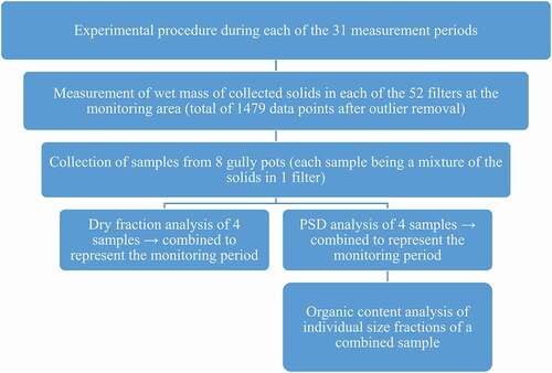
After an initial period of approximately 3 months of testing the methods, materials, and protocols, measurements were performed from April 2018 to April 2020. The filters were emptied every 3–4 weeks, both to prevent clogging of the filters and to identify the time dependency of the solids loading. An overview of the analyses during each monitoring period is provided in Figure 3.

Figure 3. Experimental procedure

Seasonal periodicity is suspected in the solids loading, in particular induced by leaf abscission from deciduous trees because of the solids’ reservoir on urban surfaces. Therefore, photos were made during the monitoring period (added as Figure S5 in the Supplementary Material) to determine the actual status of the vegetation. Following Halverson, Gleason, and Heisler (1985), four tree phases are distinguished, namely ‘leaf growth’, ‘full capacity’, ‘leaf abscission’ and ‘no leaves’.

The assessment of uncertainties in the measurements and analyses is provided in the Supplementary Material.

2.4. Solids loading

The wet masses of the collected solids are registered at the monitoring area. The dry masses were estimated by multiplying the average dry fraction with the wet mass for each gully pot. The average dry fraction for each monitoring period was determined by drying four samples, consisting of mixtures in an oven at 105 °C. This drying protocol and estimation of the dry mass are identical to the procedure followed by Butler, Thedchanamoorthy, and Payne (1992). The solids loading (kg∙day⁻¹∙ha⁻¹) is defined as follows:

(1) $L=\frac{f_d\cdot {\mathrm{\Sigma }}_i{m}_w\left(i\right)}{\mathrm{\Delta }t\cdot {\mathrm{\Sigma }}_{\mathrm{i}}A\left(i\right)}$(1)

where f_d is the dry fraction, m_w(i) the wet mass of filter i, Δt the length of the corresponding monitoring period, and A(i) the (paved) catchment area of gully pot i.

2.5. Particle size distribution

Butler, Thedchanamoorthy, and Payne (1992) subjected samples from streets and gully pots to a dry sieving procedure to obtain the Particle Size Distribution (PSD). However, this method proved to be unsuitable in this study, since it changed the PSD, mainly due to agglomeration of particles during the drying process. Instead of dry sieving, wet sieving was applied to determine the PSD.

In the work presented, sieves with mesh sizes 53, 300, 1180, 1800, 4750, 14,000 and 50,000 µm were used. With this number and type of sieves, a relatively smooth PSD curve could be obtained from the samples. The 300 and 1180 µm sieves were added after almost 1 year to improve the PSD curve, since a large mass fraction proved to be <1800 µm. After sieving the separate size fractions were dried at 105 °C, the PSD was obtained based on the dry mass. For each monitoring period, four samples were analysed, which PSDs were combined into one by the summation of the masses of each size fraction. This combined PSD is used in the article for analyses.

2.6. Organic content

The seven separate size fractions from each of the four samples used in the PSD analysis were combined into seven samples of different size fractions to analyse the organic content per size fraction. The organic content was assumed to be equal to the mass loss during a burning process in an oven at 600 °C, following the protocol by Melanen (1981).

2.7. Settling velocity

Solids transported to gully pots come in a wide variety of sizes, shapes and densities and consequently a wide variety of settling velocities. This is of importance for the settling rate of particles in gully pots, drainage pipes, etc.

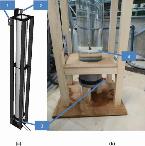
The expected settling velocity of some of these particles is relatively high. For example, the settling velocity of sand particles with a diameter of 1000 µm, quantified using the universal drag coefficient for spheres (e.g. Terfous, Hazzab, and Ghenaim 2013), is ~0.16 m/s. The particles with these relatively high settling velocities make it an unpractical task to obtain a reliable velocity distribution curve with common measurement devices, including the relatively small VICAS set-up or conventional settling columns with taps at the side. Therefore, a new settling column was developed, which is shown in Figure 4.

Figure 4. (a) Schematic drawing of the settling column. (b) Close-up of the bottom part of the settling column. 1. Switch to start measurement. 2. Weighing scale. 3. Emptying tap. 4. Dish connected to the weighing scale

Since large particles could hinder the settling of other particles, only particles <1800 µm are analysed (this sieve size was also used in the PSD analysis). This is comparable with the VICAS procedure, in which only particles <2000 µm are analysed.

Before the measurement started, the transparent column was filled from the top with water. A wet sample was carefully dropped from a cup into the column and the measurement was started simultaneously with a switch (at ‘1ʹ in Figure 4). The settling column of 2 m in height contained a disk close to the bottom of the column (at ‘4ʹ in Figure 4) which was connected with a force meter (at ‘2ʹ in Figure 4), which continuously measures the settled mass minus the buoyancy.

Since the weighing scale measured the mass of the settled particles minus the buoyancy, the variation in density should not be too large, to avoid underestimation of the mass of low-density solids. The mass is converted into a relative mass as follows:

(2) $m_{rel}{\left(t\right)}_{}=\frac{m\left(t\right)-m\left(t_0\right)}{m\left(t_{end}\right)-m\left(t_0\right)}$(2)

where m is the mass measured by the weighing scale, t₀ is the start time, and t_end is the end time of the experiment. The relative mass over time (which is smoothened with a moving median and moving average filter with a length of 1 s) is transformed into a velocity distribution curve by the following two transformations:

(3) $F_{}=\left(1-m_{rel}\right)$(3)

(4) $v=\frac{H}{t}$(4)

where F is the cumulative velocity distribution curve, v is the settling velocity and H is the height of the column. The validation of the settling column is provided in the Supplementary Material.

2.8. Rainfall

Runoff transports solids from the streets to the gully pot. Therefore, regressions are made between the solids loading and the rainfall. The rainfall data used in this article originate from the meteorological radar data set of the Royal Dutch Meteorological Institute (KNMI). This data set contains rain volume measurements on a grid with a spatial resolution of 1 km² and a temporal resolution of 5 min, which is the shortest time interval available for practical reasons. This short time interval is selected, since a gully pot catchment is relatively small, implying a short response time. As the monitoring area is relatively small, rainfall is considered to be spatially homogeneous within the area.

2.9. Temperature

The air temperature, measured at a temporal resolution of 5 min by a weather station at a distance of 4 km is used to represent the approximate average daily temperature of the environment.

2.10. Gully pot catchment area

The gully pot’s impervious catchment area is determined by application of the eight-direction flow approach (Jenson and Domingue 1988), which is required to quantify the solids loading (equation 1(1) $L=\frac{f_d\cdot {\mathrm{\Sigma }}_i{m}_w\left(i\right)}{\mathrm{\Delta }t\cdot {\mathrm{\Sigma }}_{\mathrm{i}}A\left(i\right)}$(1) ). The municipality of Rotterdam provided a data set containing laser altimetry data as measured in 2016. These measurements have a spatial resolution of 0.5 × 0.5 m². Errors in this data set caused by cars on the street have been filtered out by kriging.

3. Results and discussion

Table 1 shows a summary of the results regarding the solids loading, which are discussed in section 3.1, and the solids characteristics, which are discussed in section 3.2.

Table 1. Variation in the measured solids loading, D₅₀, organic content and settling velocity for the monitored area

Parameter	10th percentile	50th percentile	90th percentile	Unit
Solids loading	0.121	0.664	1.66	kg∙day^−1∙ha^−1
D50	0.47	0.89	11	mm
Organic content	0.26	0.41	0.70	-
vs	1.7	3.9	5.3	cm/s

3.1. Solids loading

During the monitoring campaign, spanning 737 days, a total amount of approximately 313 kg dry material was collected. The paved area connected to the gully pots was 5.300 m², resulting in a time-averaged solids loading of approximately 0.80 kg∙day⁻¹∙ha⁻¹. This number is lower than the solids deposition on the street surface, which was reported by Philippe and Ranchet (1987) to vary between 1.4 and 4.5 kg∙day⁻¹∙ha⁻¹ in residential areas in France. Possible explanations for this difference could be the removal of solids from the street by, e.g. street sweeping or wind.

On some occasions, the filters contained divergent and/or illegally dumped material, e.g. concrete, wall plaster, and paint, which was registered. Those observations and observations with values larger than three times the mean value of the corresponding monitoring period were removed during the post-processing of the data to obtain the solids loading as shown in Figure 5(b), since this graph links the solids loading to the rainfall and these materials are most likely not transported by rain. This removal of outliers reduced the data set from 1538 to 1478 observations.

Figure 5. Time dependency of the (a) rain (5-min interval) and average daily temperature, (b) solids loading, (c) D₅₀, (d) organic fraction

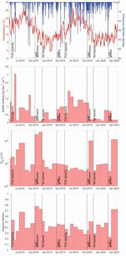
Figure 5(b) shows that the solids loading varies two orders of magnitude over the year. Most high values are observed in conjunction with the tree phases ‘leaf growth’ and ‘full capacity’ (roughly corresponding with spring and summer) in which 0.22 < L < 3.0 kg∙day⁻¹∙ha⁻¹ (except from the low solids loadings found in June 2018 and April 2020, which are likely due to a lack of rainfall in those periods). Most low values can be found during the tree phases ‘leaf abscission’ and ‘no leaves’ in which 0.051 < L < 1.2 kg∙day⁻¹∙ha⁻¹. Initially, it was assumed that the solids loading would show a peak during the ‘leaf abscission’ phase due to extra organic material available for transport, and there is increased transport of organic as will be discussed in section 3.2.2, but these materials may have such a low mass density that other processes dominate the solids loading expressed in terms of mass.

The difference between these two regimes, namely (1) during the ‘leaf growth’ and ‘full capacity’ phase and (2) during the ‘leaf abscission’ and ‘no leaves phase’, might be explained by the temperature. Figure 5(a) shows that the average daily temperature is highest during the ‘leaf growth’ and ‘full capacity’ phase. The temperature might influence the dryness of the soil and since dry soil is more prone to erosion than wet soil, the parameter ‘temperature’ might represent the erodibility of solids.

Ellis and Harrop (1984), who monitored the solids loading to gully pots in spring and summer, found the maximum solids loadings during summer and reported peak values of 1.1 kg∙day⁻¹∙ha⁻¹ in their monitoring area of 533 m² over a period of 14 days, and somewhat lower loadings (0.032 < L < 0.67 kg∙day⁻¹∙ha⁻¹) during spring. These values are in the same order of magnitude as the ones found in the current study.

Wash-off models (such as Sartor and Boyd 1972; Pitt 1979; Egodawatta, Thomas, and Goonetilleke 2007; Muthusamy et al. 2018) usually include the antecedent dry period and the rain intensity to estimate the solids loading. Since the observed parameter ‘solids loading’ is the integral of the build-up and wash-off processes over a couple of weeks, the rainfall volume could be considered as a parameter influencing the solids loading. In the current study, the solids loading proved to be correlated strongest to the rainfall intensity.

Figure 6(a) shows the solids loading versus the maximum rain intensity in the corresponding period and the markers indicate the tree phases. As previously discussed, two regimes seem to be present regarding the solids loading. Figure 6(a) suggests that the solids loading during the regime ‘leaf growth’ and ‘full capacity’ phase is correlated with the rain intensity, which is assessed in Figure 6(b) by a Monte Carlo simulation (which is described in more detail in the Supplementary Material) of a linear regression including the uncertainty in the data. The confidence interval of the regression shows that a significant, positive correlation (with R² = 0.45) exists between the solids loading and the maximum rain intensity, while a significant correlation is not present during the other regime.

Figure 6. The maximum rain intensity versus the solids loading. (a) Measurements obtained in all four tree phases. (b) The solids loading during the ‘leaf growth’ and ‘full capacity’ phase is correlated with the maximum rain intensity as indicated by the linear regression and its 95% confidence interval, which are based on a Monte Carlo simulation, which is discussed in the Supplementary Material. All displayed confidence intervals originate from the uncertainty in the measurements and their propagation, which are elaborately discussed in the Supplementary Material

3.2. Solids characteristics

3.2.1. Particle size distribution

An obvious way to characterise the collected solids is their grain size range. Solids with a size range between 53 and 1800 µm were mainly sand particles. The large solids were mainly fibres and leaves, cigarette buds, pebbles, etc. The PSDs (of which two examples are shown in Figure S4 in the Supplementary material) and therefore the D₅₀ values vary strongly over the year as shown in Figure 5(c). D₅₀ is calculated by logarithmic interpolation and varies between 420 (September 2018) and 24,000 µm (November 2018). Sansalone et al. (1998) measured (with dry sieving) 350< D₅₀ < 800 µm, Pratt and Adams (1984) 680 µm and Ellis and Harrop (1984) 600< D₅₀ < 1000 µm (both with wet sieving).

Figure 5(c) shows that the D₅₀ is large during the ‘leaf abscission’ phases, the summer of 2018 and in April 2020. This is caused by the dominance of leaves in the samples during these periods, which was to be expected for the ‘leaf abscission’ phase. The summer of 2018 and April 2020 was extraordinarily dry (Figure 5(a)), reducing the transport capacity of fine solids, while leaves could still be transported by wind. Moreover, the drought even caused deciduous trees to drop their leaves in the summer of 2018, which has been recorded in the photographs taken during sampling.

Rietveld, Clemens, and Langeveld (2020a) showed that the accumulation rate of solids in gully pots shows a maximum in terms of volume during the ‘leaf abscission’ phase, but Figure 5(b) shows that the ‘leaf abscission’ phase corresponds to the lowest solids loading. Therefore, the volume captured in the gully pot is not directly proportional to the mass inflow and the characteristics of the solids have to be taken into account, when the mass inflow is transformed into the volume captured in the gully pot.

3.2.2. Organic content

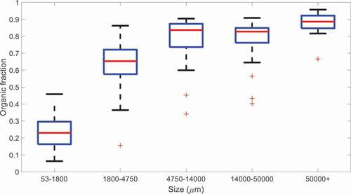
Figure 7 shows the distributions of the organic fraction per size fraction. Similar to Welker, Gelhardt, and Dierschke (2019) a positive correlation between the size and the organic fraction is observed. Welker, Gelhardt, and Dierschke (2019) found organic fractions of 0.18–0.34 for particles between 0 and 2000 µm and 0.45–0.64 for particles between 2000 and 8000 µmfor areas with high vegetation, which was distinguished by the tree canopy coverage. These values are comparable with the two smallest size fractions in Figure 7.

Figure 7. Boxplot of the organic fraction by size fraction, which indicates that the larger size fractions contain more organic material

The organic content fraction of the entire sample, which varies between 0.17 and 0.78 over the year, is shown in Figure 5(d). This broad range is comparable with the organic fraction of 0.40 to 0.70 found in street runoff in Paris (Gromaire-Mertz et al. 1999). Figure 5(d) shows that relatively large organic fractions are present during the ‘leaf abscission’ phase, the dry summer of 2018, and in April 2020. Generally, the processes influencing the D50 coincide with those related to the organic fraction over the year, which is due to the relation between the size of the solids and the organic fraction as indicated in Figure 6. Additionally, a relatively large rain volume often corresponds with an increased fraction of fine solids while fine solids hold the most inorganic material. The rain volume in the ‘leaf abscission’ phase of 2019 is relatively large, which might explain why the peak in the organic fraction in the ‘leaf abscission’ phase of 2018 is substantially larger.

Pratt and Adams (1984) found an increased organic content between October and December due to leaf abscission and between May and September due to the summer shedding of flower petals and grass cutting debris. The first finding can also be recognised in Figure 6(d), while the second is virtually absent, except for a short period in the summer of 2018 for reasons discussed earlier. This may be due to the absence of lawns and parks in the study area.

3.2.3. Settling velocity

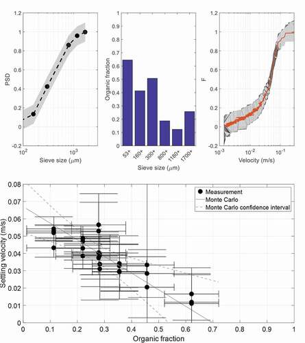
The settling velocity of the samples consisting of particles <1800 µm has been assessed with the newly designed settling column (Figure 4). Figure 8(a-c) shows the PSD, the organic fraction, and the velocity distribution of one such sample. The v₅₀ of this sample is approximately 0.04 m/s, which is comparable to the settling velocity of sand particle with a diameter of approximately 300 µm by applying the universal using the universal drag coefficient for spheres (e.g. Terfous, Hazzab, and Ghenaim 2013).

Figure 8. (a–c.) The PSD, organic fraction and velocity distribution of one sample. (d). The v₅₀ of the analysed samples is correlated with the overall organic fraction as indicated by the linear regression and its 95% confidence interval, which are based on a Monte Carlo simulation. All displayed confidence intervals originate from the uncertainty in the measurements and their propagation, which are elaborately discussed in the Supplementary Material

The removal efficiency of sand particles by a gully pot is assessed by Rietveld, Clemens, and Langeveld (2020b) in an artificial gully pot with a cross-section of 0.35 × 0.35 m² and an outlet at the opposite side of the inlet. The removal efficiency at discharges ≤1.8 L/s for sand particles with a diameter of approximately 400 µm was >75% and for particles with a diameter of approximately 180 µm was >45%. These removal rates decrease when the sediment bed level was close to the outlet pipe. A discharge of 1.8 L/s corresponds to a rain intensity of 61 mm/h, by dividing the flow rate by a virtual drained area of 106 m² (which is the mean of catchments in the monitoring area). This rain intensity occurs approximately once a year for 10 min in The Netherlands (Beersma and Versteeg 2019), so for most rainfall events higher removal efficiencies can be expected, if the sediment bed is below the outlet pipe.

The v₅₀ of the analysed samples varies relatively strongly, which cannot be explained by the slight variation in the PSD. Figure 8(d) shows that this variation can be explained by the strong variation in the organic fraction of the samples (with R² = 0.73). The organic fraction influences both the density and the shape of the particles.

4. Conclusions

This study on the solids loading to drainage systems is based on an extensive monitoring campaign compared to literature in terms of the number of gully pots sampled as well as in terms of their duration. The solids’ build-up is highly variable even within a street (Vaze and Chiew 2002), resulting in a strong variation in terms of mass and composition to individual gully pots, and consequently such a large number of sampling locations are required to represent a catchment realistically. Moreover, the solids loading strongly varies over time and can substantially differ between the same season in consecutive years. Therefore, a monitoring campaign of at least 2 years is required to capture the seasonal fluctuations.

The solids loading in the monitoring area reached a maximum during the ‘leaf growth’ and ‘full capacity’ phase, which are related to spring and summer. The highest average daily temperatures, which can be found during the same phases, might influence the erodibility of the available solids, since dry soil is more prone to erosion than wet soil. The parameter ‘rain intensity’ is correlated with the solids loading during the ‘leaf growth’ and ‘full capacity’ phase and might represent the transport capacity.

The D₅₀ and the organic fraction are correlated, since the coarse sediment fraction consists mainly of organic material. Both show a maximum during the ‘leaf abscission’ phase, the summer of 2018, and in April 2020. This is mainly due to leaves dropped by deciduous trees and the lack of rain which is the main transport driver of fine, inorganic material. The settling velocity of particles < 1800 µm ranges between 0.01 and 0.06 m/s and is strongly correlated with their organic fraction.

Acknowledgements

The authors would like to thank the municipality of Rotterdam for providing the monitoring area, providing practical assistance and for the installation of the experimental set-up.

Disclosure statement

No potential conflict of interest was reported by the author(s).

Supplementary material

Supplemental data for this article can be accessed https://doi.org/10.1080/1573062X.2021.1925706.

Additional information

Funding

The research is performed within the Dutch ‘Kennisprogramma Urban Drainage’ (Knowledge Programme Urban Drainage). The involved parties are: ARCADIS, Deltares, Evides, Gemeente Almere, Gemeente Arnhem, Gemeente Breda, Gemeente Den Haag, Gemeentewerken Rotterdam, Gemeente Utrecht, GMB Rioleringstechniek, KWR Watercycle Research Institute, Royal HaskoningDHV, Stichting RIONED, STOWA, Sweco, Tauw, vandervalk+degroot, Waterschap De Dommel, Waternet and Witteveen+Bos.

References

- Amato, F., X. Querol, C. Johansson, C. Nagl, and A. Alastuey. 2010. “A Review on the Effectiveness of Street Sweeping, Washing and Dust Suppressants as Urban PM Control Methods.” Science of the Total Environment 408 (16): 3070–3084. doi:https://doi.org/10.1016/j.scitotenv.2010.04.025.
- Ashley, R. M., D. J. Wotherspoon, M. J. Goodison, and I. Mcgregor. 1992. “The Deposition and Erosion of Sediments in Sewers.” Water Science and Technology 26 (5–6): 1283–1293. doi:https://doi.org/10.2166/wst.1992.0571.
- Ashley, R. M., R. W. Crabtree, A. Fraser, and T. Hvitved-Jacobsen. 2003. “European Research into Sewer Sediments and Associated Pollutants and Processes.” Journal of Hydraulic Engineering 129 (4): 267–275. doi:https://doi.org/10.1061/(ASCE)0733-9429(2003)129:4(267).
- Beersma, J., and R. Versteeg. 2019. Basisstatistiek Voor Extreme Neerslag in Nederland [Statistics of Extreme Rainfall in the Netherlands]. Amersfoort: STOWA.
- Bertrand-Krajewski, J. L., P. Briat, and O. Scrivener. 1993. “Sewer Sediment Production and Transport Modelling: A Literature Review.” Journal of Hydraulic Research 31 (4): 435–460. doi:https://doi.org/10.1080/00221689309498869.
- Bonhomme, C., and G. Petrucci. 2017. “Should We Trust Build-p/Wash-off Water Quality Models at the Scale of Urban Catchments?” Water Research 108: 422–431. doi:https://doi.org/10.1016/j.watres.2016.11.027.
- Boogaard, F. C., F. Van de Ven, J. G. Langeveld, and N. Van de Giesen. 2014. “Stormwater Quality Characteristics in (Dutch) Urban Areas and Performance of Settlement Basins.” Challenges 5 (1): 112–122. doi:https://doi.org/10.3390/challe5010112.
- Butler, D., S. Thedchanamoorthy, and J. A. Payne. 1992. “Aspects of Surface Sediment Characteristics on an Urban Catchment in London.” Water Science and Technology 25 (8): 13–19. doi:https://doi.org/10.2166/wst.1992.0174.
- Butler, D., and S. H. P. G. Karunaratne. 1995. “The Suspended Solids Trap Efficiency of the Roadside Gully Pot.” Water Research 29 (2): 719–729. doi:https://doi.org/10.1016/0043-1354(94)00149-2.
- Crabtree, R. W. 1989. “Sediment in Sewers.” Water and Environment Journal 3 (6): 569–578. doi:https://doi.org/10.1111/j.1747-6593.1989.tb01437.x.
- De Man, H. 2014. “Best Urban Water Management Practices to Prevent Waterborne Infectious Diseases under Current and Future Scenarios.” PhD Thesis., University of Utrecht.
- Deletic, A., and D. W. Orr. 2005. “Pollution Buildup on Road Surfaces.” Journal of Environmental Engineering 131 (1): 49–59. doi:https://doi.org/10.1061/(ASCE)0733-9372(2005)131:1(49).
- Droppo, I. G., K. N. C. K. J. Irvine, E. Carrigan, S. Mayo, C. Jaskot, and B. Trapp. 2006. “26 Understanding the Distribution, Structure and Behaviour of Urban Sediments and Associated Metals toward Improving Water Management Strategies.” In Soil Erosion and Sediment Redistribution in River Catchments: Measurement, Modelling and Management. Wallingford: CABI Publishing.
- Egodawatta, P., E. Thomas, and A. Goonetilleke. 2007. “Mathematical Interpretation of Pollutant Wash-off from Urban Road Surfaces Using Simulated Rainfall.” Water Research 41 (13): 3025–3031. doi:https://doi.org/10.1016/j.watres.2007.03.037.
- Ellis, J. B., B. Chocat, J. Fujita, J. Marsalek, and W. Rauch. 2004. Urban Drainage. London: IWA Publishing.
- Ellis, J. B., and D. O. Harrop. 1984. “Variations in Solids Loadings to Roadside Gully Pots.” Science of the Total Environment 33 (1–4): 203–211. doi:https://doi.org/10.1016/0048-9697(84)90394-2.
- Ellis, J. B., and T. Hvitved-Jacobsen. 1996. “Urban Drainage Impacts on Receiving Waters.” Journal of Hydraulic Research 34 (6): 771–783. doi:https://doi.org/10.1080/00221689609498449.
- Furumai, H., H. Balmer, and M. Boller. 2002. “Dynamic Behavior of Suspended Pollutant and Particle Size Distribution in Highway Runoff.” Water Science and Technology 46 (11–12): 413–418. doi:https://doi.org/10.2166/wst.2002.0771.
- Gelhardt, L., M. Huber, and A. Welker. 2017. “Development of a Laboratory Method for the Comparison of Settling Processes of Road-deposited Sediments with Artificial Test Material.” Water, Air, and Soil Pollution 228 (12): 467. doi:https://doi.org/10.1007/s11270-017-3650-8.
- Gromaire-Mertz, M. C., S. Garnaud, A. Gonzalez, and G. Chebbo. 1999. “Characterisation of Urban Runoff Pollution in Paris.” Water Science and Technology 39 (2): 1–8. doi:https://doi.org/10.1016/S0273-1223(99)00002-5.
- Grottker, M. 1990. “Pollutant Removal by Gully Pots in Different Catchment Areas.” Science of the Total Environment 93: 512–522. doi:https://doi.org/10.1016/0048-9697(90)90142-H.
- Halverson, H. G., S. B. Gleason, and G. M. Heisler. 1985. “Leaf Duration and the Sequence of Leaf Development and Abscission in Northeastern Urban Hardwood Trees.” Urban Ecology 9: 323–335. doi:https://doi.org/10.1016/0304-4009(86)90007-0.
- Herngren, L. F. 2005. Build-up and Wash-off Process Kinetics of PAHs and Heavy Metals on Paved Surfaces Using Simulated Rainfall. Brisbane: Queensland University of Technology.
- Hixon, L. F., and R. L. Dymond. 2018. “State of the Practice: Assessing Water Quality Benefits from Street Sweeping.” Journal of Sustainable Water in the Built Environment 4: 3. doi:https://doi.org/10.1061/JSWBAY.0000860.
- Hong, Y., C. Bonhomme, L. Minh-Hoang, and G. Chebbo. 2016. “A New Approach of Monitoring and Physically-based Modelling to Investigate Urban Wash-off Process on A Road Catchment near Paris.” Water Research 102: 96–108. doi:https://doi.org/10.1016/j.watres.2016.06.027.
- Jenson, S. K., and J. O. Domingue. 1988. “Extracting Topographic Structure from Digital Elevation Data for Geographic Information System Analysis.” Photogrammetric Engineering and Remote Sensing 54 (11): 1593–1600.
- Lau, S. L., and M. K. Stenstrom. 2005. “Metals and PAHs Adsorbed to Street Particles.” Water Research 39 (17): 4083–4092. doi:https://doi.org/10.1016/j.watres.2005.08.002.
- McKenzie, E. R., and T. M. Young. 2013. “A Novel Fractionation Approach for Water Constituents - Distribution of Storm Event Metals.” Environmental Science: Processes Impacts 15: 1006–1016. doi:https://doi.org/10.1039/C3EM30612G.
- Melanen, M. 1981. Quality of Runoff Water in Urban Areas. Helsinki: National Board of Waters.
- Muthusamy, M., S. Tait, A. Schellart, M. N. A. Beg, R. F. Carvalho, and J. L. De Lima. 2018. “Improving Understanding of the Underlying Physical Process of Sediment Wash-off from Urban Road Surfaces.” Journal of Hydrology 557: 426–433. doi:https://doi.org/10.1016/j.jhydrol.2017.11.047.
- Naves, J., J. Anta, J. Suárez, and J. Puertas. 2019. “WASHTREET - Hydraulic, Wash-off and Sediment Transport Experimental Data Obtained in an Urban Drainage Physical Model.” Zenodo. doi:https://doi.org/10.5281/zenodo.3233918.
- Philippe, J. P., and J. Ranchet. 1987. Pollution des Eaux de Ruissellement Pluvial en Zone Urbaine. Synthèse des Mesures sur Dix Bassins Versants en Région Parisienne [Pollution of Rainwater Runoff in Urban Areas. Summary of Measures on Ten Watersheds in the Paris Region]. Paris: Laboratoire Central des Ponts et Chaussées.
- Pitt, R. 1979. Demonstration of Nonpoint Pollution Abatement through Improved Street Cleaning Practices. Washington DC: U.S. EPA.
- Pitt, R., D. Williamson, J. Voorhees, and S. Clark. 2005. “Review of Historical Street Dust and Dirt Accumulation and Washoff Data.” Journal of Water Management Modeling. doi:https://doi.org/10.14796/JWMM.R223-12.
- Pitt, R., S. Clark, V. K. Eppakayala, and R. Sileshi. 2017. “Don’t Throw the Baby Out with the Bathwater - Sample Collection and Processing Issues with Particulate Solids in Stormwater.” Journal of Water Management Modeling. doi:https://doi.org/10.14796/JWMM.C416.
- Pratt, C. J., and J. R. W. Adams. 1984. “Sediment Supply and Transmission via Roadside Gully Pots.” Science of the Total Environment 33 (1–4): 213–224. doi:https://doi.org/10.1016/0048-9697(84)90395-4.
- Rietveld, M. W. J., F. H. L. R. Clemens, and J. G. Langeveld. 2020a. “Monitoring and Statistical Modelling of the Solids Accumulation Rate in Gully Pots.” Urban Water Journal 17 (6): 549–559. doi:https://doi.org/10.1080/1573062X.2020.1800760.
- Rietveld, M. W. J., F. H. L. R. Clemens, and J. G. Langeveld. 2020b. “Solids Dynamics in Gully Pots.” Urban Water Journal 17 (7): 669–680. doi:https://doi.org/10.1080/1573062X.2020.1823430.
- Saget, A., G. Chebbo, and J. L. Bertrand-Krajewski. 1996. “The First Flush in Sewer Systems.” Water Science & Technology 33 (9): 101–108. doi:https://doi.org/10.1016/0273-1223(96)00375-7.
- Sansalone, J., J. J. Koran, J. M. Smithson, and S. G. Buchberger. 1998. “Physical Characteristics of Urban Roadway Solids Transported during Rain Events.” Journal of Environmental Engineering 124 (5): 427–440. doi:https://doi.org/10.1061/(ASCE)0733-9372(1998)124:5(427).
- Sartor, J. D., and G. B. Boyd. 1972. Water Pollution Aspects of Street Surface Contaminants. Washington DC: U.S.EPA.
- Simperler, L., K. Keckeis, and T. Ertl 2019. “Using a Solids Mass Balance Model for Impact Estimation of Stormwater Management Measures on Sewer Operation.” Proceedings of the 9th International Conference on Sewer Processes & Networks, Aalborg, Denmark.
- Terfous, A., A. Hazzab, and A. Ghenaim. 2013. “Predicting the Drag Coefficient and Settling Velocity of Spherical Particles.” Powder Technology 239: 12–20. doi:https://doi.org/10.1016/j.powtec.2013.01.052.
- Van Bijnen, M., H. Korving, J. G. Langeveld, and F. H. L. R. Clemens. 2018. “Quantitative Impact Assessment of Sewer Condition on Health Risk.” Water 10 (3): 245. doi:https://doi.org/10.3390/w10030245.
- Vaze, J., and S. Chiew. 2002. “Experimental Study of Pollutant Accumulation on an Urban Road Surface.” Urban Water 4 (4): 379–389. doi:https://doi.org/10.1016/S1462-0758(02)00027-4.
- Walker, T. A., and T. H. F. Wong. 1999. Effectiveness of Street Sweeping for Stormwater Pollution Control. Melbourne: Cooperative Research Centre for Catchment Hydrology.
- Welker, A., L. Gelhardt, and M. Dierschke. 2019. “Vegetation and Temporal Variability of Particle Size Distribution (PSD) and Organic Matter of Urban Road Deposited Sediments in Frankfurt Am Main.” Proceedings of Novatech 2019, Lyon, France.
- Xanthopoulos, C., and A. Augustin. 1992. “Input and Characterization of Sediments in Urban Sewer Systems.” Water Science and Technology 25 (8): 21–28. doi:https://doi.org/10.2166/wst.1992.0175.
- Zafra, C. A., J. Temprano, and I. Tejero. 2008. “Particle Size Distribution of Accumulated Sediments on an Urban Road in Rainy Weather.” Environmental Technology 29 (5): 571–582. doi:https://doi.org/10.1080/09593330801983532.