Optimisation of pumping and storage design through iterative hydraulic adjustment for minimum energy consumption

ABSTRACT

Water distribution networks (WDNs) require large capital investment and ongoing operational costs, resulting in their optimisation being a highly researched field. Despite the benefits tanks bring to networks, most optimisation models omit them as decision variables due to the complexity they can introduce to heuristic approaches. This paper addresses the least-cost optimisation of WDN design and operation through the development and application of the Small-network Configurator for Optimising Pump Energy consumption (SCOPE). The SCOPE algorithm incorporates pipes, pumps and tanks as decision variables and solves the optimisation problem through an iterative approach that pairs EPANET simulation results with subsequent hydraulic calculations to converge on the pumping and storage configuration which yields the lowest energy consumption. The SCOPE output can then be used to seed further optimisation techniques. This approach has been tested on the synthetic Nametown and real-life Dili networks and demonstrated annual cost savings of 10% and 25%, respectively.

KEYWORDS:

• Pumping and storage configuration
• genetic algorithm (GA)
• design and operation optimisation
• lifetime least-cost
• water distribution networks

Introduction

Water Distribution Networks (WDNs) typically represent the most significant component of a water utility’s total assets (Moneim, 2011; VEWIN, 2017). Furthermore, the operation of most WDNs requires substantial expenditure, predominantly consisting of electricity costs associated with pump energy consumption within the network (Giacomello, Kapelan, and Nicolini, 2013). Therefore, the optimisation of WDNs (both design and operation) presents water utilities a significant opportunity to minimise cost and maximise performance.

WDN optimisation problems are inherently complex and nonlinear in nature due to their combinatorial set of components and hydraulic behaviour (Verleye and Aghezzaf, 2016). The advancement of computational processing power has facilitated the use of higher-level optimisation techniques such as evolutionary algorithms (EAs), multi-method searching and hyper-heuristics to optimise WDNs (Mala-Jetmarova, Sultanova, and Savic, 2017).

A review of existing literature conducted by Mala-Jetmarova et al., (2017) found that the relative majority (41%) of 288 papers focussed on the optimisation of WDN design and noted that tanks were often omitted as decision variables, despite the multiple benefits they bring to a WDN (Batchabani and Fuamba, 2014). Furthermore, research efforts that focus on the operational optimisation of WDNs are typically framed as pump scheduling problems for existing infrastructure which, again, neglects tanks as decision variables. Therefore, this paper aims to contribute to the emerging set of optimisation problems concerned with minimising WDN cost over its design life (capital and operational expenditure) by incorporating tanks as decision variables. The novelty of the approach presented lies in configuring the decision variables associated with pumping station design (duty head, duty flow and variable speed pattern), tank design (location, elevation and volume) and operation (initial level, minimum and maximum levels) for a given network by iterative, incremental hydraulic adjustment whilst adhering to minimum performance levels (minimum nodal head and maximum allowable unit headloss in pipes). The optimal tank location is determined by assessing all possible locations and returning the location which produces the lowest capital and operational expenditure (CAPEX and OPEX) after a net present value (NPV) calculation. This is obtained by iteratively simulating a tank connected at every node in combination with the associated pumping station design such that its flow rate is fixed at the network’s average daily demand (and thus, consumes the least energy for that tank location). As the presented methodology does not simultaneously solve for all WDN decision variables, the result yielded cannot be said to be the global optimum, however, it approaches the global optimum by returning the pumping and storage configuration which produces the minimum pumping energy consumption for the network without changing its pipe diameters unless a critical unit headloss is exceeded. For this reason, the approach lends itself to pre- and post-processing to further refine the network which is explored further in the methodology section. The result is an algorithm capable of processing real-life WDN problems where system configuration and operation are both optimised with limited computational resources. Furthermore, it is one of the few methodologies which incorporates the decision variables associated with tank design into the optimisation procedure to minimise pump energy consumption (Batchabani and Fuamba, 2014).

The layout of the paper is as follows: the introduction is succeeded by a background information section that reviews the current state of literature concerning the optimisation of WDNs over its entire lifecycle by including tanks as decision variables. The methodology section follows and describes the development of SCOPE – the Small-network Configurator for Optimising Pump Energy consumption. This tool is then applied to two cases: a synthetic network (case study 1) and the real-life network of Dili, Timor-Leste (case study 2). The results are discussed observing SCOPE’s advantages and limitations. Finally, the conclusions and recommendations for further research are noted.

Background

Approximately 60% of literature optimisation models have pipe diameters as their only decision variable despite WDNs being made up of pipes, pumps, tanks and valves over an almost infinitely variable geometry and configuration (Mala-Jetmarova et al., 2017). With gradually increasing computational power at their disposal, researchers have begun to integrate pumps, tanks and valves into their optimisation models. Pumps and tanks have an interdependent relationship and their configuration and interaction influences both capital and operational cost. As such, they should be considered simultaneously to optimise WDNs to reach the best solution for the total economic cost (Walters et al., 1999). The primary advantage of water storage is balancing the peaks and troughs of the demands placed on the network, water treatment facilities and raw water abstraction. Consequently, the capacity of each component in the entire raw water abstraction → water treatment → water distribution chain may be reduced, presenting significant capital and operational savings to the water utility. Secondary advantages of incorporating water storage within a network include stabilised system pressures and water reserves which can ensure continuous supply in extreme events such as fires, pipeline bursts and power outages.

Water storage can be positioned as either in- or on-ground reservoirs or elevated tanks. Elevated tanks are subject to engineering economy feasibility limits which restrict their capacity to approximately 9,000 m³ (Krug and Ghadban, 2004), whereas in- or on-ground reservoirs are not limited in volume. Water in elevated storage tanks ‘floats’ on the connected network’s hydraulic grade line, which facilitates indirect pumping – a supply regime where a pump is disconnected from responding to the network’s daily demand profile through the flow balancing functionality the tank provides. Conversely, direct pumping meets 100% of the network’s demands in real time through the pump which is governed by the dynamic system curve of the network. In- or on-ground reservoirs can also behave as floating tanks, provided they are located at strategic points in the topographical landscape with sufficient elevation. Krug and Ghadban, (2004) note that indirect pumping in combination with floating storage offers the following advantages over direct pumping: i) reduces pumping peaks, ii) stabilises pressures in response to fluctuating demands, iii) provides reliable water supply at constant pressure, iv) prevents contaminating inflow at pipe leaks and joints by ensuring consistently elevated pressures, v) facilitates levelling of pumped flow at average daily demand, vi) eliminates the need for a wide range of pump sizes, vii) reduces pumping costs – especially if the electricity provider implements a peak/off-peak price structure, viii) piping to the tank needs only to be designed for average network flow instead of peak flow, ix) provides immediate response to calamities such as pipe bursts and power outages, x) delivers immediate firefighting flows and pressures and xi) dampens hydraulic transients caused by surging or water hammer.

Krug and Ghadban, (2004) go on to identify the potential degradation of water quality as the primary drawback of water storage. This can be due to increased residence time in tanks, additional water stagnation within non-recirculation areas within tanks, the development of biofilms on tank walls and contamination risks. Compared to direct pumping alone, other disadvantages associated with water storage include: i) land cost within cities may be prohibitively expensive/challenging to procure, ii) may be aesthetically displeasing, iii) require labour for regular cleaning, iv) potential variations in water age, v) vulnerable to natural disasters, such as earthquakes and hurricanes, vi) prone to freezing in extremely cold climates, vii) water unpalatable and prone to biological growth at high temperatures in extremely hot climates and viii) vulnerable to security issues such as vandalism and terrorism.

The extent to which previous least-cost optimisation studies have considered tanks in their optimisation problem depends on either the tank parameters that have been included as decision variables or fixing different tank scenarios to investigate the effect on the optimisation process (Stokes, Maier, and Simpson, 2016). The simplest form of incorporating tanks into the optimisation problem involves a binary decision variable for a tank of known parameters as performed on the Anytown network by Johns et al., (2014). Tanks can also be included as discrete decision variables for specifying location only (Wu, Simpson, and Maier, 2010) and integer decision variables for sizing and location (Fu et al., 2013). However, to fully design a tank the following parameters need to be specified: a) location, b) length and diameter of the riser, c) minimum and maximum operational level, d) emergency volume, e) top level, f) shape and g) height/diameter ratio (Vamvakeridou-Lyroudia, Walters, and Savic, 2005). Except for the location, all other parameters are used to determine the tank volume at certain moment in time, which is then used as a key decision variable in a heuristic optimisation problem. The tank shape can be specified later based on common engineering knowledge.

Optimisation methods which include tanks as decision variables started with linear programming gradient (LPG) methods (Alperovits and Shamir, 1977) and nonlinear programming generalised reduced gradient methods (Lansey and Mays, 1989) before trending towards heuristic methods, corresponding with the increased computational power available by the late 20th century. The most common heuristic methods are variations of evolutionary algorithms (EAs) such as Genetic Algorithms (GA) (Dandy and Hewitson, 2000; Murphy, Dandy, and Simpson, 1994; Ostfeld, 2005; Prasad, 2010; Rogers et al., 2009; Savic and Walters, 1997; Vamvakeridou-Lyroudia, Walters, and Savic, 2005), Non-dominated Sorting Genetic Algorithms (NSGA-II) (Basupi and Kapelan, 2015; Fu et al., 2013; Stokes, Simpson, and Maier, 2015; Wu, Simpson, and Maier, 2008, 2010) and Borg multi-objective evolutionary algorithms (Borg MOEA) (Stokes, Maier, and Simpson, 2016). Less common heuristic methods include Ant Colony Optimisation (ACO) methods such as the one employed by Shokoohi et al., (2017) where tank heads were incorporated into the multi-objective optimisation problem as a decision variable. However, the above heuristic approaches used in WDN optimisation are computationally expensive, and their search space can become unfeasibly large with a high number of decision variables.

To address this issue, heuristic methods have been simplified by employing a hybrid approach. Research efforts have incorporated traditional analytical approaches within heuristic approaches which take advantage of their computational efficiency to reduce the size of the search space, thus improving the overall optimisation performance (Haghighi, Samani, and Samani, 2011; Krapivka and Ostfeld, 2009; Loganathan, Greene, and Ahn, 1995; Zheng, Simpson, and Zecchin, 2011). Owing to new optimisation solvers offering increased computational efficiency, more recent research has returned to using traditional analytical approaches exclusively such as the iterative LP-NLP method introduced by Qiu et al., (2020) or the hybrid type combinations of the heuristic and traditional methods (Giacomello, Kapelan, and Nicolini, 2013). These methods demonstrate several advantages compared to heuristic methods including increased robustness in the face of increasing loading conditions, parameter tuning is no longer required and decreased computational burden. The Qiu et al., (2020) approach was further developed into a tri-stage method, by introducing a middle step in the two-stage process which converted the split-pipe design output of the first LP stage to discrete, commercially available pipe diameters before applying the final NLP stage which established the new flow distribution which minimises the WDN operational cost (Qiu, Housh, and Ostfeld, 2021).

The research presented in this paper offers an alternative to analytical and heuristic optimisation methods through the development of the less computationally demanding SCOPE algorithm that utilises incremental hydraulic adjustment based on hydraulic model (i.e. EPANET) simulation results to optimise the pumping and storage configuration. The SCOPE results are then post processed using a single-objective, single-constraint Genetic Algorithm to optimise the pipe diameters. Similar methodologies have proven to be successful, such as Kandiah et al., (2012) who won 3^rd place in the Battle of the Water Networks II (BWN-II) (Marchi et al., 2014) by utilising a Genetic Algorithm to optimise the Anytown network in which their level of effort for manual pre-processing was classified as three out of a maximum of four. Kandiah et al., (2012) utilised an engineering approach to develop an initial solution to the BWN-II design problem and then further refined the optimisation procedure by reducing the decision variables to 396 (down from an estimated 4,000) prior to submitting to a GA for processing. In contrast, the SCOPE-based methodology omits the need for engineering judgement to reduce the decision variables prior to GA application by establishing the pumping and storage configuration which yields the lowest energy consumption. This removes tank location, tank elevation, tank balancing volume (BV), pump duty flow, pump duty head and pump variable speed pattern prior to processing with a subsequent GA, greatly simplifying the optimisation procedure.

Hydraulic relationship between storage and pumps

The role and basic hydraulic operation of pumps and tanks is well known. Yet, their individual design will largely depend on their interactions in the network, which has implications on the formulation of the optimisation problem setup. These implications are briefly elaborated on in this section.

To achieve all the benefits that balancing storage tanks bring to a network, they must be correctly sized to balance the full daily demand variation. If a tank’s BV is undersized causing a net loss of water at the end of a 24-hour period, the capacity of the network’s pumps may be exceeding during the subsequent peaks in demand, resulting in inadequate service levels to consumers. Therefore, the final tank level at the end of the day should be equal to or greater than the initial tank level, thus preventing loss of water over a longer period. Based on this condition, the theoretical BV can be graphically determined by plotting the cumulative water demand and supply profiles and taking the sum of the two greatest distances between the curves. Smet et al., (2002) demonstrates this concept in Figure 1 for a given network demand profile and three different pumping scenarios. The pumping scenarios are two 6-hour, 12-hour and 24-hour constant rate pumping, and their corresponding BV can be graphically calculated by BV = C’-C”+D’-D”, BV = C’-C+D-D’ and BV = A-A’+B-B’. The required balancing volumes in this example are approximately 76%, 22% and 28% of the network’s daily demand for scenarios 1, 2 and 3, respectively. The BV can also be calculated numerically as per Equation 12.(12) $\begin{array}{c}BV=\mathrm{\Delta }t\cdot \left(\sum _{t=0}^{t_{max}}\left(Q_{in}-Q_{out}\right)+\left|\sum _{t=0}^{t_{min}}\left(Q_{in}-Q_{out}\right)\right|\right)\end{array}$(12) In practice, complex networks make it difficult to achieve 100% balancing and therefore the correction of tank levels is regularly achieved by (automatic) adjustment of pumping schedules. These adjustments can, however, result in additional energy costs on account of underutilised BV, labelled ‘demand balancing volume’ in Figure 2. As tank functioning is intrinsically linked to the pumping scheme supplying the network, each pumping scheme produces a unique BV that satisfies the network’s demand pattern. Thus, to minimise the costs, the optimisation problem must be defined with attention to both the BV size and the pumping schedule.

Figure 1. Graphical determination of required storage volume (Smet et al., 2002).

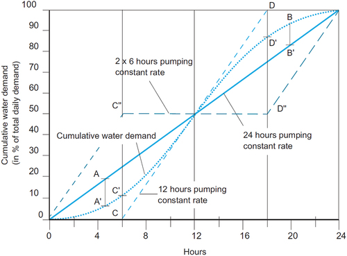
Figure 2. Water storage volume composition (Trifunović 2020b).

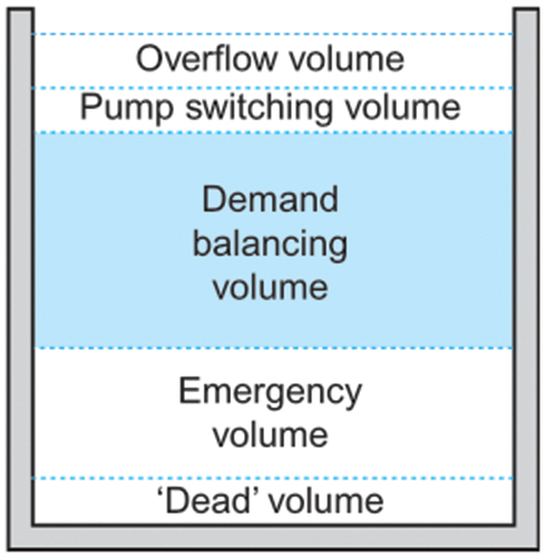
In addition to BV, tank volume consists of other provisions, namely: emergency, overflow, pump switching and ‘dead’ volumetric components, as shown in Figure 2. The emergency volume is the second major provision for extraordinary conditions such as power outages, pipe bursts or firefighting load. Some risk assessments will be used for design purposes, but in practice, the emergency volume is often constrained by construction feasibility and water quality problems arising from extended periods of stagnation. Therefore, it is rarely selected as decision variable in WDN optimisation.

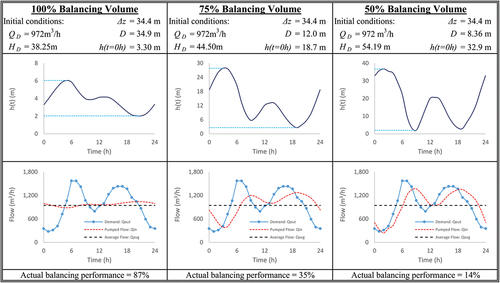
Of the three pumping schemes shown in Figure 1, the constant rate pumping over the 24-hour duration yields the lowest pump energy consumption as the BV of the tank facilitates the lowest constant flow rate from the pump. Unnecessary increase in pumping will automatically result in underutilisation of the BV. On the other hand, if the available BV is less than 100% of the network’s required BV, the pumped flow rate will tend to increase towards the direct pumping case with the peaks and troughs smoothed out by the operation of the tank. The extent to which the tank can smoothen the variation in demand is a function of its volume, leading to a hypothesis that there is a relationship between the BV in a network and the pump energy consumption; both of which contribute cost components (tanks predominantly capital cost and pump energy consumption exclusively operational cost) to the total cost that should be minimised.

The above is illustrated in Figure 3, where a numerical hydraulic model (MS Excel) was set up to investigate the effect of incrementally reducing the utilised BV of a tank from 100% to 50% by reducing its diameter. The model is hypothetical as it allows the water level in the tank to reach unrealistic heights to reduce the utilised BV by effectively throttling the pump without implementing pump controls. The numerical model was initialised with the following inputs: Δz = tank height above the pump, D = tank diameter, h(t = 0 h) = tank initial level, Q_D = pump duty flow and H_D = pump duty head. Reducing the tank diameter and increasing the pump duty head such that the tank final level equalled the initial level after 24 hours had the effect of forcing the pump to respond to a greater portion of the instantaneous demand without implementing pump controls. The subsequent response is shown below the corresponding tank functioning for volumes 100%, 75% and 50% of the total BV. It can be observed that even in the case of 100% BV available, the pump response is influenced by the variable head imparted on the pump due to the changing water level in the tank. The ‘Actual Balancing Performance’ of the tank can be described as the percentage of BV minus the area under Q_avg which is bounded by Q_in and will tend towards 100% as Q_in approaches Q_avg. As the utilised BV reduces, the pumped flow, Q_in, tends towards the daily demand profile, gradually emulating the direct pumping supply scenario, i.e. increasing the pumping energy consumption.

Figure 3. Tank and pump response to 100%, 75% and 50% of network balancing volume.

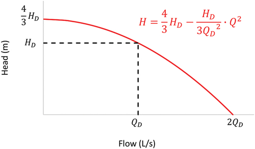
The simple example above demonstrates that the maximised utilisation of BV can only be achieved with constant pump operation at the average daily demand, which, in turn, results in the lowest energy consumption. However, actual pump operation typically varies in response to the varying pressures and demands of the network, as governed by its pump characteristic curve. As such, to minimise the pumping costs, it is necessary to introduce a variable speed pump (VSP) and controls to ensure constant operation. Furthermore, the pump can be designed such that its point of maximum operational efficiency coincides with the average daily demand. EPANET, the application for modelling drinking water distribution systems developed by Rossman, (2000), can be used to model constant pump operation at its point of maximum efficiency by first modelling its pump characteristic curve as a single-point pump curve, where a head-flow combination which represents a pump’s desired operating point is defined by duty head, H_D, and duty flow, Q_D. This relationship is governed by the following equation and the corresponding pump curve as shown in Figure 4 (Rossman, 2000):

Figure 4. Single-point pump curve for duty head, H_D, and duty flow, Q_D adapted from Rossman, (2000b).

(1) $\begin{array}{c}H=\frac{4}{3}{H}_D-\frac{H_D}{3{Q_D}^2}\cdot Q^2\end{array}$(1)

Following pump and network set up, hydraulic simulations in EPANET can then be used to plot the pressure profile experienced by the pump throughout a 24-hour extended period simulation (EPS). From this, a pump speed setting can be calculated using the pump affinity laws shown in the following equations:

(2) $\begin{array}{c}\frac{Q_1}{Q_2}=\frac{N_1}{N_2}\end{array}$(2)

(3) $\begin{array}{c}\frac{H_1}{H_2}={\left(\frac{N_1}{N_2}\right)}^2\end{array}$(3)

where N₁ gives the pump speed multiplier with respect to its default speed, by setting N₂  = 1. Equation 1(1) $\begin{array}{c}H=\frac{4}{3}{H}_D-\frac{H_D}{3{Q_D}^2}\cdot Q^2\end{array}$(1) , Equation 2(2) $\begin{array}{c}\frac{Q_1}{Q_2}=\frac{N_1}{N_2}\end{array}$(2) and Equation 3(3) $\begin{array}{c}\frac{H_1}{H_2}={\left(\frac{N_1}{N_2}\right)}^2\end{array}$(3) can be manipulated to derive an expression for pump speed, N(t), which produces the average daily demand, Q_avg, for the head at each time step, t, during the day.

This is done by substituting H = H₂ and Q = Q₂ in Equation 1(1) $\begin{array}{c}H=\frac{4}{3}{H}_D-\frac{H_D}{3{Q_D}^2}\cdot Q^2\end{array}$(1) , then rearranging Equation 2(2) $\begin{array}{c}\frac{Q_1}{Q_2}=\frac{N_1}{N_2}\end{array}$(2) and Equation 3(3) $\begin{array}{c}\frac{H_1}{H_2}={\left(\frac{N_1}{N_2}\right)}^2\end{array}$(3) to form an expression for Q₂² which is then back substituted into Equation 1(1) $\begin{array}{c}H=\frac{4}{3}{H}_D-\frac{H_D}{3{Q_D}^2}\cdot Q^2\end{array}$(1) and Equation 3(3) $\begin{array}{c}\frac{H_1}{H_2}={\left(\frac{N_1}{N_2}\right)}^2\end{array}$(3) in order to obtain Equation 4.(4) $\begin{array}{c}{N}_1=\sqrt{\frac{3{Q_D}^2{H}_1+H_D{Q_1}^2}{4H_D{Q_D}^2}}\end{array}$(4)

(4) $\begin{array}{c}{N}_1=\sqrt{\frac{3{Q_D}^2{H}_1+H_D{Q_1}^2}{4H_D{Q_D}^2}}\end{array}$(4)

Recognising that fixing Q_D = Q_avg ensures that the selected pump operates at its highest efficiency and letting N₁ = N(t) and H₁ = H(t) to obtain a general expression of pump speed as a function of time step, t, the above expression for N₁ simplifies to:

(5) $\begin{array}{c}N\left(t\right)=\sqrt{\frac{1}{4}+\frac{3H\left(t\right)}{4H_D}}\end{array}$(5)

which can be used to compute the VSP pattern. This pattern will force the pump to operate at its theoretical highest efficiency point, Q_D, across the day.

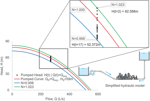
The above is illustrated in Figure 5 for a simplified hydraulic model, where the standard pump characteristic curve, shown in red, is moved up or down as required by altering the VSP speed setting, N(t), for each time step. The green and blue curves show the maximum and minimum speeds that the pump is required to operate, where N = 1.023 at 17:00 hours, and N = 0.956 at 02:00 hours, respectively. The relatively low range of pressures results in a narrow range of pump speeds, whereas the range of fluctuating pressures is likely to be larger in real-world cases, justifying VSP selection.

Figure 5. Variable speed setting, N, such that pump operates at average flow, Q_D.

Methodology

Problem statement

The optimal design of WDNs incorporating tanks should provide a least-cost solution over the infrastructure’s lifetime whilst ensuring nodal demands are met with sufficient pressure. Using simplified engineering economy approach demonstrated by Trifunović, (2020a, 2020b), this can be expressed by minimising Total Annual Expenditure (TAE) as follows:

(6) $\begin{array}{c}MinimiseTAE=\frac{\left(Cp+Cv+Ct+Cpu\right)\cdot r}{1-{\left(1+r\right)}^{-n}}+Mp+Mv+Mt+Mpu+Opu\end{array}$(6)

where Cp, Cv, Ct and Cpu represent the capital expenditure of the network’s pipes, valves, tanks and pumps, respectively. The loan conditions required to service the capital costs are given by r (annual interest rate) and n (number of annual repayments). Mp, Mv, Mt and Mpu indicate the annual maintenance costs associated with the network’s pipes, valves, tanks and pumps, while the final term Opu captures the energy cost drawn by the pumps within the network.

The above optimisation objective function (Equation 6(6) $\begin{array}{c}MinimiseTAE=\frac{\left(Cp+Cv+Ct+Cpu\right)\cdot r}{1-{\left(1+r\right)}^{-n}}+Mp+Mv+Mt+Mpu+Opu\end{array}$(6) ) is subject to the following constraints:

(7) $\begin{array}{c}{H}_i\ge H_{i,min}fori=1,\dots ,NJ\end{array}$(7)

(8) $\begin{array}{c}{S}_j=\frac{\mathrm{\Delta }{h}_j}{L}\end{array}$(8)

(9) $\begin{array}{c}{S}_j\le S_{j,max}forj=1,\dots ,NP\end{array}$(9)

(10) $\begin{array}{c}T{L}_{\left(t=0\right)}\le T{L}_{\left(t=24\right)}\end{array}$(10)

(11) $\begin{array}{c}{\sigma }_{pumped}=\sqrt{\frac{1}{24}\sum _{t=1}^{24}{\left(Q_{pumped\left(t\right)}-Q_{avg}\right)}^2}<{\sigma }_{allowable}\end{array}$(11)

where each node i (of total number of junctions, NJ) must have a minimum head greater than the minimum pressure requirement, H_min. The unit head loss, S_j, in each pipe j (of total number of pipes, NP) must be less than the maximum unit head loss requirement (S_max). The tank final level, TL_(t = 24), must be equal to or greater than the tank initial level, TL_(t = 0), to prevent water loss over an extended period. Finally, the standard deviation of the pumped flows, σ_pumped, from the average pumped flow, which is equal to the average daily demand, Q_avg must be less than σ_allowable to enforce pump operation within acceptable tolerance from Q_avg. In addition to the aforementioned constraints, the optimisation problem is also subject to the physical constraints: i) conservation of flow and ii) conservation of mass which are handled by EPANET’s hydraulic engine.

The decision variables are (1) tank location, (2) tank elevation, (3) tank BV, (4) pump duty flow, (5) pump duty head, (6) pump variable speed pattern and (7) commercially available pipe diameters. Other variables that form input into optimisation problem but are not optimised are tank emergency volume, tank initial level, tank diameter and tank maximum level. These are set based on common engineering practice.

Solution method

The above optimisation problem is to be solved for the network’s maximum daily demand profile to ensure system redundancy for lower consumption days, using the following procedure:

1. Pre-processing: WDN partitioning into network segments modelled with one pump and one reservoir with no pressure reducing valves (PRVs) to ensure compatibility with SCOPE.

2. SCOPE application: Network segments submitted for processing by SCOPE to return the VSP and tank configuration which yields the lowest pump energy consumption at the location coinciding with the lowest CAPEX and OPEX.

3. Post-processing: A single-objective implementation of a GA is applied post SCOPE processing to further optimise the pipe diameters.

The above steps are required to be executed independently and are further elaborated in the following sections.

Pre-processing (WDN partitioning)

In SCOPE’s current form, it is limited to processing small networks which consist of one pump, one source (modelled as a reservoir in EPANET) and no PRVs. This limitation can be bypassed by partitioning larger networks into smaller network segments which comply with SCOPE’s requirements. Networks with multiple pumps are to be partitioned by summing all the nodal demands upstream of the pump and adding them into the last node prior to the pump. The network segments downstream of the pump are to be removed from the original network and modelled as a standalone network by replacing the node prior to the pump with a reservoir with a total head equal to the minimum total head that the intake side of the pump experienced during the entire network’s extended period simulation (EPS). Finally, all PRVs are to be removed from the network model segments prior to submission to SCOPE for processing. While SCOPE is not suitable for all networks, it can be applied to more complex networks containing pumps supplying segments which can be modelled on their own, as shown in Case Study 2.

SCOPE application

The Small-network Configurator for Optimising Pump Energy (SCOPE) is a heuristic algorithm that produces a network with the pumping and storage configuration with the minimum energy consumption whilst adhering to the hydraulic constraints outlined in Equation 7(7) $\begin{array}{c}{H}_i\ge H_{i,min}fori=1,\dots ,NJ\end{array}$(7) to Equation 11(11) $\begin{array}{c}{\sigma }_{pumped}=\sqrt{\frac{1}{24}\sum _{t=1}^{24}{\left(Q_{pumped\left(t\right)}-Q_{avg}\right)}^2}<{\sigma }_{allowable}\end{array}$(11) . As the minimum pressure constraint (Equation 7(7) $\begin{array}{c}{H}_i\ge H_{i,min}fori=1,\dots ,NJ\end{array}$(7) ) can only be met by increasing either the pumping head, the static head contribution from water level within the tank or by enlarging pipe diameters for a given network, SCOPE systematically converges on these parameters through incremental hydraulic adjustment until it reaches its stopping criteria (defined by Equation 7(7) $\begin{array}{c}{H}_i\ge H_{i,min}fori=1,\dots ,NJ\end{array}$(7) to Equation 11(11) $\begin{array}{c}{\sigma }_{pumped}=\sqrt{\frac{1}{24}\sum _{t=1}^{24}{\left(Q_{pumped\left(t\right)}-Q_{avg}\right)}^2}<{\sigma }_{allowable}\end{array}$(11) ) and moves to the next parameter. As SCOPE’s functionality to adjust pipe diameters is limited to enlarging pipes which exceed a maximum headloss threshold (Equation 9(9) $\begin{array}{c}{S}_j\le S_{j,max}forj=1,\dots ,NP\end{array}$(9) ), the algorithm’s output cannot be said to be the theoretical global optimum of the network. However, for a network of given pipe diameters it establishes the tank location, tank elevation, tank BV, pump duty flow, pump duty head and pump variable speed pattern which yields the minimum pump energy consumption. Therefore, SCOPE is ideally suited as a precurser to network optimisation through the application of evolutionary algorithms as it greatly reduces the search space by heuristically determining the aforementioned decision variables.

SCOPE was developed by using the Python programming language in conjunction with the Water Network Tool for Resilience (WNTR), an open-source Python package developed by Klise et al., (2017). The SCOPE flowchart is shown in Figure 6. The key steps of this method are as follows:

Figure 6. SCOPE flowchart.

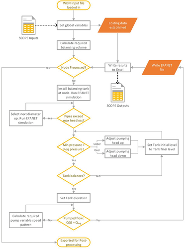
1. SCOPE loads an EPANET input file and then prompts the user to specify the remaining inputs: 1) pipe installation cost table, 2) uniform roughness value for new pipes, 3) minimum nodal pressure, 4) maximum allowable unit head loss, 5) balancing tank minimum and maximum levels, 6) typical power outage duration (used to size the emergency volume portion of the tank), 7) tank connection length and diameter, 8) global pump efficiency, 9) allowable standard deviation of pumped flow from average, 10) energy price, 11) operation and maintenance rates and 12) loan interest rate and repayment period. The basic costing framework applied with the financial input parameters follows the approach presented by Trifunović, (2020a, b).

2. SCOPE calculates the demand balancing volume, BV, based on the graphical method of plotting the cumulative water demand and supply profiles (refer Figure 1) over 24 hours by taking the sum of the two greatest distances between the curves as per Equation 12(12) $\begin{array}{c}BV=\mathrm{\Delta }t\cdot \left(\sum _{t=0}^{t_{max}}\left(Q_{in}-Q_{out}\right)+\left|\sum _{t=0}^{t_{min}}\left(Q_{in}-Q_{out}\right)\right|\right)\end{array}$(12) shown below:

   (12) $\begin{array}{c}BV=\mathrm{\Delta }t\cdot \left(\sum _{t=0}^{t_{max}}\left(Q_{in}-Q_{out}\right)+\left|\sum _{t=0}^{t_{min}}\left(Q_{in}-Q_{out}\right)\right|\right)\end{array}$(12)

where Q_in = Q_avg = tank inflow (m³/h), Q_out = tank outflow (m³/h), Δt = Extended Period Simulation timestep, $t_{max}=t\mathrm{s}\mathrm{u}\mathrm{c}\mathrm{h}\mathrm{t}\mathrm{h}\mathrm{a}\mathrm{t}\mathrm{m}\mathrm{a}\mathrm{x}\left\{\mathrm{\Delta }t\cdot \sum _1^t\left(Q_{in}-Q_{out}\right):t=1,\cdots ,24\right\}$ and $t_{min}=t\mathrm{s}\mathrm{u}\mathrm{c}\mathrm{h}\mathrm{t}\mathrm{h}\mathrm{a}\mathrm{t}\mathrm{m}\mathrm{i}\mathrm{n}\left\{\mathrm{\Delta }t\cdot \sum _1^t\left(Q_{in}-Q_{out}\right):t=1,\cdots ,24\right\}$. 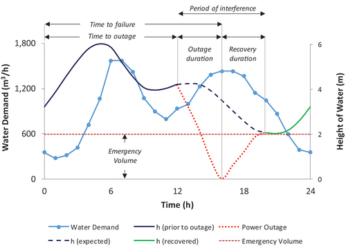The emergency volume, EV, is calculated in a similar manner to Equation 12(12) $\begin{array}{c}BV=\mathrm{\Delta }t\cdot \left(\sum _{t=0}^{t_{max}}\left(Q_{in}-Q_{out}\right)+\left|\sum _{t=0}^{t_{min}}\left(Q_{in}-Q_{out}\right)\right|\right)\end{array}$(12) with Q_in being modified to Q_in = Q_avg prior to power outage | 0 during power outage |Q_{pump max} after a power outage (m³/h) until recovery occurs as shown in Figure 7 and computed with Equation 13.(13) $\begin{array}{c}EV=\mathrm{\Delta }t\cdot \left(\sum _{t=0}^{t_{max}}\left(Q_{in}-Q_{out}\right)+\left|\sum _{t=0}^{t_{min}}\left(Q_{in}-Q_{out}\right)\right|\right)-BV\end{array}$(13)

Figure 7. Example balancing tank response to a 4h power outage.

(13) $\begin{array}{c}EV=\mathrm{\Delta }t\cdot \left(\sum _{t=0}^{t_{max}}\left(Q_{in}-Q_{out}\right)+\left|\sum _{t=0}^{t_{min}}\left(Q_{in}-Q_{out}\right)\right|\right)-BV\end{array}$(13)

Equation 13(13) $\begin{array}{c}EV=\mathrm{\Delta }t\cdot \left(\sum _{t=0}^{t_{max}}\left(Q_{in}-Q_{out}\right)+\left|\sum _{t=0}^{t_{min}}\left(Q_{in}-Q_{out}\right)\right|\right)-BV\end{array}$(13) is performed for the nominated power outage duration starting at every timestep in a 24-hour period to determine the EV required to ensure continuous supply should the power outage occur during the most vulnerable time of the day. To illustrate this step, an example tank response to a 4-hour power outage is shown in Figure 7. SCOPE then calculates the required tank diameter using the minimum and maximum levels (user input 5) which yields a total volume of BV + EV.

(3) SCOPE then sets the source pump duty flow equal to the average demand and configures the EPANET model’s global pump efficiency (user input 8) and energy price (user input 10). SCOPE then commences to loop over every node in the network and connect the tank (as sized in step 2) to the node which is the subject of the current loop iteration via a pipe of nominated length, diameter and roughness (user inputs 2 and 7). SCOPE connects the tank such that it fills and empties from the bottom, resulting in the connected node experiencing pressure variations as a function of tank water level. This is aligned to EPANET’s modelling procedure for tanks. SCOPE then saves out each network after it has been hydraulically configured to produce the lowest pump energy consumption such that there will be NJ networks (Number of Junctions) with one tank connected to the subject node of the current loop iteration. Figure 8 graphically depicts the method with quasi code that SCOPE undertakes to configure each network hydraulically in which it performs a series of nested loops to incrementally adjust the following key parameters:

Figure 8. Graphical representation of SCOPE’s step 3 procedure with quasi code.

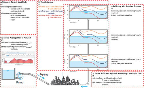
1. Firstly, SCOPE runs a demand driven EPANET simulation with the tank connected to the current node and checks that the network has sufficient hydraulic conveying capacity to the tank location by checking that each pipe, for NP, does not exceed the maximum unit headloss threshold (Equation 9(9) $\begin{array}{c}{S}_j\le S_{j,max}forj=1,\dots ,NP\end{array}$(9) ). If a pipe exceeds this threshold, it is enlarged to the next commercially available diameter specified in the pipe installation cost table (user input 1).

2. Secondly, SCOPE ensures that 100% of the tank’s BV is utilised by raising or lowering the tank initial level based on the tank final level at the end of the 24-hour EPANET simulation (Equation 10(10) $\begin{array}{c}T{L}_{\left(t=0\right)}\le T{L}_{\left(t=24\right)}\end{array}$(10) ). Figure 8 (graphic b) depicts tank response that is losing water (red line) and gaining water (yellow line) which can be corrected to be balanced (blue line) at this step.

3. SCOPE’s third nested loop raises or lowers the pump duty head and tank elevation such that the node which experiences the lowest pressure within the EPANET simulation is equal to the minimum nodal pressure (user input 3). This ensures that the minimum pressure constraint (Equation 7(7) $\begin{array}{c}{H}_i\ge H_{i,min}fori=1,\dots ,NJ\end{array}$(7) ) is not violated. Figure 8 (graphic c) depicts three tank elevations of which the middle corresponds to the elevation and pump duty head which satisfies the minimum pressure requirement.

4. Within the loops above, SCOPE employs Equation 5(5) $\begin{array}{c}N\left(t\right)=\sqrt{\frac{1}{4}+\frac{3H\left(t\right)}{4H_D}}\end{array}$(5) to compute the pump’s variable speed pattern which will result in the pump operating at its Duty Flow, Q_avg. This step calculates the standard deviation, σ_pumped, of the pump’s actual flow, Q(t), and if the result is greater than σ_allowable (user input 9) SCOPE will recompute the VSP pattern (Equation 11(11) $\begin{array}{c}{\sigma }_{pumped}=\sqrt{\frac{1}{24}\sum _{t=1}^{24}{\left(Q_{pumped\left(t\right)}-Q_{avg}\right)}^2}<{\sigma }_{allowable}\end{array}$(11) ).

5. Upon completion of steps a, b, c and d, the network can be considered as configured to consume the lowest energy consumption for the tank connected to the subject node. The final EPANET simulation is used to record the hydraulic performance of the network. SCOPE calculates the CAPEX and OPEX for this network configuration and then moves onto the next node in the original network until all the nodes have been processed.

(4) Finally, SCOPE saves the modified EPANET configuration with the tank location and pump duty head that produce the least energy consumption along with the calculated Total Annual Expenditure (TAE given by Equation 6(6) $\begin{array}{c}MinimiseTAE=\frac{\left(Cp+Cv+Ct+Cpu\right)\cdot r}{1-{\left(1+r\right)}^{-n}}+Mp+Mv+Mt+Mpu+Opu\end{array}$(6) ) and publishes the results to Excel. The results can be sorted by TAE in ascending order to identify the location of the tank which produces the least-cost design.

Post-processing (pipe diameter optimisation)

At the end of the SCOPE application, the pumping and storage configuration is established, i.e. the following decision variables are determined: (1) tank location, (2) tank elevation, (3) tank BV, (4) pump duty flow, (5) pump duty head, (6) pump variable speed pattern and (7) pipe diameters (which originally exceeded Equation 9)(9) $\begin{array}{c}{S}_j\le S_{j,max}forj=1,\dots ,NP\end{array}$(9) . These results can be used to seed heuristic approaches to further optimise pipe diameters. To demonstrate this, Hadka’s, (2019) implementation of a single-objective, single-constraint Genetic Algorithm has been employed to optimise the pipe diameters of the SCOPE processed network governed by Equation 6(6) $\begin{array}{c}MinimiseTAE=\frac{\left(Cp+Cv+Ct+Cpu\right)\cdot r}{1-{\left(1+r\right)}^{-n}}+Mp+Mv+Mt+Mpu+Opu\end{array}$(6) and Equation 7(7) $\begin{array}{c}{H}_i\ge H_{i,min}fori=1,\dots ,NJ\end{array}$(7) . The genetic operators selected were as follows: population size = 100, generator = random generator, selector = tournament selector of size 2, crossover = half-uniform crossover and mutator = bitflip mutation where Hadka’s (2019) default threshold probabilities for crossover and mutation were utilised (Holland 1992).

Case study 1: Nametown network

Description

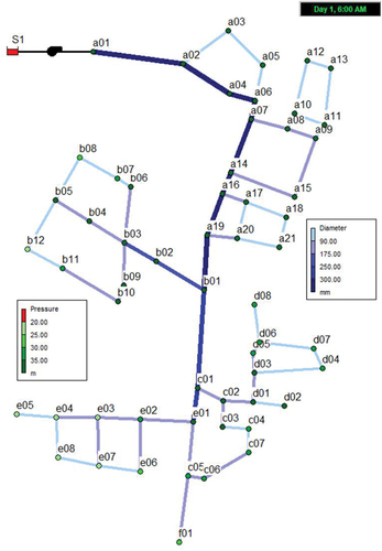
SCOPE was first tested on the adapted Nametown network (Trifunović 2020a) shown in Figure 9, which is supplied via a direct pumping regime (i.e. no tank). The EPANET network model consists of 57 nodes supplied from a single source, labelled ‘S1’, through a semi-looped configuration. The minimum pressure and maximum allowable unit head loss were chosen at 20 mwc and 10 m/km, respectively. An energy price of 0.15 EUR/kWh and a 20-year loan repayment period at 6% interest per annum were selected as inputs of the SCOPE costing model. The original Nametown network was modified to emulate a fully flat topography by setting all the nodal elevations to zero in order to investigate the optimal balancing tank location for a network subject only to friction losses, i.e. amplifying the influence of network resistance.

Figure 9. Nametown network layout (most critical node: e05 = 20.08 mwc @ 6:00 AM), adapted from Trifunović (2020b).

Results

Based on the applied diurnal patterns and assuming constant supply from the source, the total theoretical BV of 1,470 m³ required for the network was calculated (Equation 12(12) $\begin{array}{c}BV=\mathrm{\Delta }t\cdot \left(\sum _{t=0}^{t_{max}}\left(Q_{in}-Q_{out}\right)+\left|\sum _{t=0}^{t_{min}}\left(Q_{in}-Q_{out}\right)\right|\right)\end{array}$(12) ) using the principles illustrated in Figure 1. With the emergency storage set at 1,110 m³, the combined storage volume of 2,580 m³ should ensure continuity of water supply in response to the assumed 3-hour power outage at the most vulnerable time of 16:00 hours; a moment when the tank is at emergency volume during regular supply. Based on this total volume, a tank height of 6 m and minimum level of 2.58 m were selected based on engineering judgement and input into the SCOPE algorithm (user input 5) which subsequently calculated the tank diameter to be 23.4 m to meet the network’s storage needs.

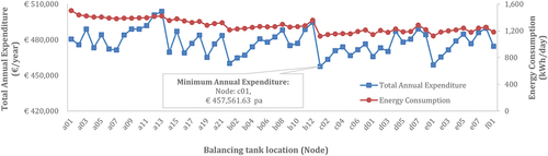
With the designed balancing tank tested at each node, SCOPE processed the network in under 5 minutes on a standard laptop (Intel® Core™ i5 with 4 GB RAM) and produced 57 hydraulically solved networks. Using the lifetime least-cost framework, SCOPE found the optimal tank location at node c01, resulting in a total annual expenditure of EUR 458,000, as shown in Figure 10. This result represents a 5% cost saving compared to the original network without the balancing tank. The optimal balancing tank location coincided with the location which yields the lowest pumping energy. The authors note that this may not always be the case, especially in networks with electricity block tariff structures.

Figure 10. Nametown SCOPE processed results for total annual expenditure and pumping energy consumption for each possible tank location.

With the SCOPE determined 7 decision variables set, the resultant network lends itself to post-processing with GA to further optimise the pipe diameters. With the pipe diameters as the only decision variable and the minimum pressure requirement as the only constraint, the complexity of the GA is greatly reduced. The GA post-processing of Nametown with the balancing tank located at node c01, was executed in 110 minutes on a standard laptop. The results are summarised in Table 1 (where the GA post-processing yields a further 5% reduction in total annual expenditure for a total of EUR 435,000) and the resultant pipe diameters are displayed in Figure 11 along with the SCOPE determined VSP pattern. Using the GA as a post-processing tool on the SCOPE optimised network returns a combined saving in the total annual expenditure of EUR 47,000, representing a total saving of 10% compared to the original Nametown network.

Figure 11. Optimised decision variables where (a) shows the SCOPE determined pump variable speed pattern, (B) shows the SCOPE determined tank position and pipe diameters and (C) shows GA post-processed pipe diameters.

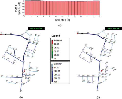
Table 1. Decision variables and resultant financial summary for SCOPE and GA post-processed Nametown network (in EUR).

Decision Variable/Cost Component			Network Variant
			Nametown - Original	SCOPE-Processed	GA Post-Processed
Decision Variable	Tank Location		-	c01	c01
	Tank Elevation		-	26.6m	26.6m
	Tank Balancing Volume		-	1,470m^3	1,470m^3
	Tank Emergency Volume		-	1,110m^3	1,110m^3
	Pump Duty Flow		540m^3/h	370m^3/h	370m^3/h
	Pump Duty Head		65m	34.8m	34.8m
	Pump Variable Speed Pattern		-	Refer Figure 11 (A)	-
	Pipe Diameters		Refer Figure 9	Refer Figure 11 (B)	Refer Figure 11 (C)
Cost Component	CAPEX	Pipes	2,434,649	2,584,543	2,243,529
		Pumping Station	1,227,730	907,505	907,505
		Tank	-	637,818	637,818
		Sub-Total	3,662,379	4,129,866	3,788,852
		Loan Repayment	319,303	360,061	330,329
	OPEX	Operation	126,388	61,326	69,717
		Maintenance	36,728	36,175	35,084
Total Annual Expenditure			482,419	457,562	435,130

Case study 2: dili network

Description

The EPANET model of the proposed WDN of Dili (Timor-Leste), as developed by Seureca Veolia (2016), consists of 264 junctions, 5 water sources, 13 storage tanks, 298 pipes, 5 pumping stations and 41 valves. Using the same engineering economy approach proposed by Trifunović, (2020a, b) and shown in Equation 6(6) $\begin{array}{c}MinimiseTAE=\frac{\left(Cp+Cv+Ct+Cpu\right)\cdot r}{1-{\left(1+r\right)}^{-n}}+Mp+Mv+Mt+Mpu+Opu\end{array}$(6) , the baseline cost of the future WDN of Dili comprises a total annual cost of USD 6.60 M, as shown in Table 2. This model network was selected as case study to test SCOPE because i) it is slated for replacement by 2030 and the new network is currently in the design phase, ii) Timor-Leste, being a developing nation, is subject to high electricity costs and frequent power outages making the incorporation of tanks within the network critical to its performance. Thus, the optimisation of the pumping and storage within the network would bring tangible benefits to the people of Dili. Preliminary runs of the model reflected a well-designed network from a hydraulic perspective, with most nodal pressures between 20 and 60 mwc. Still, 14% of the nodes have their pressure below the minimum of 20 mwc considered as adequate service level. Furthermore, 6% of the Dili WDN pipes exceed the unit head loss threshold of 10 m/km according to the simulation results.

Table 2. Baseline cost for the proposed Dili WDN (in USD).

Component	CAPEX	OPEX			Annual Expenditure
		Loan Repayment	Energy Consumption	Maintenance
Pipes	20,590,793	1,795,199	-	102,954	1,898,153
Valves	588,040	51,268	-	-	51,268
Tanks	7,123,919	621,096	-	56,991	678,087
Pumping stations	3,638,923	317,258	3,585,843	72,778	3,975,880
Total Annual Expenditure:					6,603,388

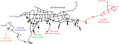
In line with SCOPE’s limitations, the Dili WDN was partitioned into six network segments which complied with the one source and one pump requirement as displayed in Figure 12 Using EPANET water quality simulations to trace the sources allowed further simplification by removal of minor water sources which gravity-fed the Dili Main network segment. Dili Main was excluded from SCOPE application because it is gravity-fed and thus has no benefit of pumping energy optimisation. Further adaptation included modelling a source reservoir on the intake side of the pump supplying each network segment with a total head equal to the minimum pressure head observed in the node connected to the pump intake in the full-scale network EPS.

Figure 12. Partitioned Dili WDN.

Dili RHS main SCOPE results

The SCOPE algorithm was used to process all the segments depicted in Figure 12 (excluding Dili Main) and was followed by post-processing as described in the methodology section of this paper. However, for brevity, only the results for the individual network segment Dili RHS Main are shown here.

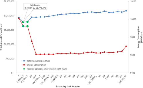
SCOPE took less than 5 minutes of computational time to process the network. The results for total annual expenditure and energy consumption for each possible tank location are shown in Figure 13. As it can be seen from this figure, the tank’s optimal location is at node ‘R_HERA_2’ with a height of 17.1 m above ground. The node ‘R_HERA_2’ is a zero-demand node placed in EPANET to facilitate the connection of a tank at the natural ridgeline in the topography. Therefore, the minimum pressure requirement of 20 mwc does not apply to this node, and the tank can be placed on the ground rather than atop an elevated structure of 17.1 m (which when combined with the 2.9 m emergency volume satisfies the minimum pressure requirement). Due to the Dili RHS Main network’s topography, this is only one of two feasible nodes at which the tank can be connected and the construction height is kept under 50 m.

Figure 13. Dili RHS Main network SCOPE results.

Table 3 compares the pre- and post-SCOPE application parameters and produces a capital and operational cost saving of approximately USD 53,000 and USD 1.45 M, respectively. The large operational cost savings arises from a human error in the original network design where the duty head of the pump was approximately double what it needed to be. This excess head was then wasted at a PRV downstream.

Table 3. Comparison of the original and SCOPE processed parameters for the Hera pumping station.

Hera Summary	Original Configuration	SCOPE Optimised	Cost Savings
Duty Flow (m^3/h)	750	724
Duty Head (m)	300	157
Annual Energy Consumption (kWh/year)	7,070,044	3,626,555
Pump Investment Cost (USD)	1,948,035	1,894,725	−53,310
Annual Energy Cost (USD)	2,969,419	1,523,153	−1,446,266
Annual O&M Cost (USD)	38,961	37,894	−1,066
Total Annual Savings:			−1,500,642

Dili RHS Main post-processing results

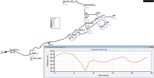
The Dili RHS Main segment consists of 30 pipes with a total length of approximately 21 km. The GA optimisation required 10,000 generations to converge on the optimal pipe diameters and took 10 minutes to execute. As a result, the optimised pipe diameters require a capital investment of USD 2.59 M compared to USD 3.80 M for the original network representing a total capital expenditure saving of USD 1.21 M. Furthermore, this CAPEX saving translates to an overall lower lifetime cost saving of USD 2.31 M due to lower loan repayments. As the minimum pressure constraint of 20 mwc is not violated (which can be seen in Figure 14, where the most critical node, J132, experiences a minimum pressure of 20.43 mwc at 08:00 hours), the GA optimised network represents a near-optimal design from an investment perspective.

Figure 14. Dili RHS Main SCOPE + GA post-processed pressure distribution.

Creating the optimised Dili WDN

Following the optimisation process, the Dili WDN (with its individually optimised segments reconnected) is shown in Figure 15. This figure shows the optimal location of the Dili network’s balancing tanks with their volumes calculated to balance the network and provide coverage for a 3-hour power outage. Additional parameters such as critical pipe diameters (pipes which exceed the maximum unit headloss constraint, Equation 9)(9) $\begin{array}{c}{S}_j\le S_{j,max}forj=1,\dots ,NP\end{array}$(9) , duty head, duty flow and variable speed pattern of the pumps, as determined by SCOPE, have also been updated into the optimised model of the Dili WDN. Table 4 presents a cost summary for the SCOPE processed Dili WDN with a bottom-line annual cost of USD 5.14 M, which translates to a 22% reduction from the original annual cost of USD 6.60 M. These savings can be extrapolated out over the 20-year payback period of the Dili network to a saving of USD 29 M.

Figure 15. Optimal location of the Dili network’s balancing tanks, as determined by SCOPE.

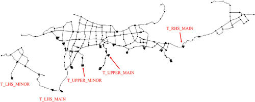
Table 4. SCOPE optimised Dili network financial summary (in USD).

Component	CAPEX	OPEX			Annual Expenditure
		Loan Repayment	Energy Consumption	Maintenance
Pipes	20,852,258	1,817,995	-	104,261	1,922,256
Valves	529,480	46,162	-	-	46,162
Tanks	8,069,914	703,572	-	64,559	768,131
Pumping stations	3,113,037	271,409	2,071,802	62,261	2,405,471
Total Annual Expenditure:					5,142,021

Table 5 displays the estimated pipe costs for the post-processed (i.e. further GA optimised network), where the total capital investment cost is USD 1.89 M cheaper than that of the SCOPE processed Dili WDN (USD 4 M over 20-year loan payback period). A slight increase in annual energy consumption can be observed and is due to the reduced (optimised) pipe diameters. However, the pump, tank and valve investment costs remain unchanged. Thus, the SCOPE application yields annual savings of 22%, which, when combined with the additional 3% from the GA parameters, totals annual savings of 25% compared to the original Dili network (USD 31 M over a 20-year loan payback period).

Table 5. GA optimised Dili network financial summary (in USD).

Component	CAPEX	OPEX			Annual Expenditure
		Loan Repayment	Energy Consumption	Maintenance
Pipes	18,996,000	1,656,158	-	94,980	1,751,138
Valves	529,480	46,162	-	-	46,162
Tanks	8,069,914	703,572	-	64,559	768,131
Pumping stations	3,113,037	271,409	2,074,078	62,261	2,407,748
Total Annual Expenditure:					4,973,179

Discussion

The SCOPE-based methodology introduced here cannot guarantee attainment of the global optimum, as it sequentially optimises different parameters, and it involves WDN segmentation in the case of more complex networks. However, SCOPE has been shown to produce the pumping and storage configuration for a network of given pipe diameters which produces the lowest energy consumption at the least-cost tank location. The subsequent optimisation of pipe diameters with a GA can then be said to obtain near-optimal pipe diameters for the given SCOPE processed network. It is worth noting that the Dili network is significantly more complex than some test networks which optimisation methods have been tested on in the literature, such as Anytown in the Battle of the Water Networks II (Marchi et al., 2014) and that the methodology presented in this paper still showed significant benefit (25% total annual savings). These results can be said to approach the global optimum design as they are demonstratively better than the base network. As the theoretical global optimum design is subject to the accuracy of the engineering economy model, future demand forecasting and growth of the network it is impossible to quantify the SCOPE-based results against the theoretical global optimum with a 100% confidence level. The results show that SCOPE is a proven tool that can handle the complexities of real-world networks while delivering tangible savings to the practising engineer based on the hydraulic principles presented in this paper. The authors acknowledge that the Dili network required significant pre-processing prior to the application of SCOPE, most notably in the form of partitioning the network into suitable segments. Distinct advantages that the SCOPE and GA optimisation procedures offer over other methods in literature are that the design and operation of network are optimised simultaneously to produce a least-cost network (CAPEX and OPEX) over a given planning horizon. Furthermore, it is one of the few methodologies within the body of literature on WDN optimisation that can accurately return the decision variables associated with tank design (location, elevation and BV) to produce a network with minimum pump energy consumption.

Conclusion

This paper presents a new SCOPE-based methodology for the optimisation of WDN configuration and operation. The methodology starts with pre-processing complex networks into segments, followed by the application of the new SCOPE method that optimises the pumping and storage configuration which yields the lowest energy consumption. This solution can then be used to seed a Genetic Algorithm (or other heuristic optimisation) based model to further optimise pipe diameters.

The new methodology was successfully applied to and demonstrated on the synthetic Nametown and real-life Dili networks, resulting in total annual savings of 10% and 25%, respectively, when compared to the original networks. Therefore, the end result is a WDN with near-optimal configuration and operation based on sound engineering principles obtained in a computationally fast manner (minutes rather than hours or days).

The limitations of SCOPE-based WDN optimisation methodology include the requirements of networks having to be supplied from one source by one pump, and without any PRVs in the model. Additionally, SCOPE does not possess the functionality to split the entire network’s balancing volume over multiple locations, which may or may not present a lower lifetime cost. However, this problem can be bypassed by adopting a sectored approach where complex networks are partitioned into smaller sub-networks, and then optimised independently.

Recommendations for future research include expanding SCOPE’s functionality to enable splitting the entire network’s balancing volumes over multiple locations and sources. Another area identified for further work includes combining SCOPE and the GA to allow the algorithm to accept pipe diameters as decision variables. This would enable the selection of larger pipe diameters to reduce the pump energy consumption, possibly leading to an overall least-cost design. As the SCOPE-based methodology optimises WDNs based on the demand profile of their maximum consumption day, further investigation is needed to understand the year-round energy implications. Additionally, the pumping regime could be further refined in response to dynamic electricity prices if SCOPE was expanded to account for block tariffs. Future works could also be undertaken to upgrade SCOPE to a multi-objective algorithm to include water age to combat the issue of water quality degradation in tanks. Furthermore, in the context of climate change, the authors believe that the further development of SCOPE’s costing model to include penalties for GHG emissions would be beneficial. Finally, future studies may wish to build a probability density function based on local conditions into the algorithm which calculates the required emergency storage volume to express water supply continuously for a known percentage of power outages.

Acknowledgement

The first author would like to thank The Rotary Foundation and their local Rotary sponsor, The Rotary Club of Manningham City.

Disclosure statement

No potential conflict of interest was reported by the authors.

Data availability statement

All data, models and code that support the findings of this study are available from the first author upon reasonable request.

Additional information

Funding

This work was supported by the Rotary Foundation under Grant GG1988998.

References

- Alperovits, E., and U. Shamir. 1977. “Design of Optimal Water Distribution Systems.” Water Resources Research 13 (6): 885–900. Wiley Online Library. https://doi.org/10.1029/WR013i006p00885.
- Basupi, I., and Z. Kapelan. 2015. “Flexible Water Distribution System Design Under Future Demand Uncertainty.” Journal of Water Resources Planning and Management 141 (4): 04014067. American Society of Civil Engineers. https://doi.org/10.1061/(ASCE)WR.1943-5452.0000416.
- Batchabani, E., and M. Fuamba. 2014. “Optimal Tank Design in Water Distribution Networks: Review of Literature and Perspectives.” Journal of Water Resources Planning and Management 140 (2): 136–145. American Society of Civil Engineers. https://doi.org/10.1061/(ASCE)WR.1943-5452.0000256.
- Dandy, G., and C. Hewitson. 2000. “Optimizing Hydraulics and Water Quality in Water Distribution Networks Using Genetic Algorithms.” Building Partnerships 1–10. https://doi.org/10.1061/9780784405178.
- Fu, G., Z. Kapelan, J. R. Kasprzyk, and P. Reed. 2013. “Optimal Design of Water Distribution Systems Using Many-Objective Visual Analytics.” Journal of Water Resources Planning and Management 139 (6): 624–633. American Society of Civil Engineers. https://doi.org/10.1061/(ASCE)WR.1943-5452.0000311.
- Giacomello, C., Z. Kapelan, and M. Nicolini. 2013. “Fast Hybrid Optimization Method for Effective Pump Scheduling.” Journal of Water Resources Planning and Management 139 (2): 175–183. American Society of Civil Engineers (ASCE). https://doi.org/10.1061/(asce)wr.1943-5452.0000239.
- Hadka, D. 2019. Platypus: Multiobjective Optimization in Python.
- Haghighi, A., H. M. V. Samani, and Z. M. V. Samani. 2011. “GA-ILP Method for Optimization of Water Distribution Networks.” Water Resources Management 25 (7): 1791–1808. https://doi.org/10.1007/s11269-011-9775-4.
- Holland, J. H. 1992. “Genetic Algorithms.” Scientific American 267 (1): 66–73. https://doi.org/10.1038/scientificamerican0792-66.
- Johns, M. B., E. Keedwell, and D. Savic. 2014. “Adaptive Locally Constrained Genetic Algorithm for Least-Cost Water Distribution Network Design.” Journal of Hydroinformatics 16 (2): 288–301. IWA Publishing. https://doi.org/10.2166/hydro.2013.218.
- Kandiah, V., M. Jasper, K. Drake, M. E. Shafiee, M. Barandouzi, A. D. Berglund, E. D. Brill, G. Mahinthakumar, S. Ranjithan, and E. Zechman. 2012. “Population-Based Search Enabled by High Performance Computing for BWN-II Design.” In WDSA 2012: 14th Water Distribution Systems Analysis Conference, 536–550, 24-27 September 2012, Adelaide, South Australia.
- Klise, K. A., D. Hart, D. Moriarty, M. L. Bynum, R. Murray, J. Burkhardt, and T. Haxton. 2017. Water Network Tool for Resilience (WNTR) User Manual.
- Krapivka, A., and A. Ostfeld. 2009. “Coupled Genetic Algorithm—Linear Programming Scheme for Least-Cost Pipe Sizing of Water-Distribution Systems.” Journal of Water Resources Planning and Management 135 (4): 298–302. American Society of Civil Engineers. https://doi.org/10.1061/(ASCE)0733-9496(2009)135:4(298).
- Krug, J., and Z. Ghadban. 2004. Mitigating the Impacts of Elevated Water Storage Tanks on Water Quality.
- Lansey, K. E., and L. W. Mays. 1989. “Optimization Model for Water Distribution System Design.” Journal of Hydraulic Engineering 115 (10): 1401–1418. American Society of Civil Engineers. https://doi.org/10.1061/(ASCE)0733-9429(1989)115:10(1401).
- Loganathan, G. v, J. J. Greene, and T. J. Ahn. 1995. “Design Heuristic for Globally Minimum Cost Water-Distribution Systems.” Journal of Water Resources Planning and Management 121 (2): 182–192. American Society of Civil Engineers. https://doi.org/10.1061/(ASCE)0733-9496(1995)121:2(182).
- Mala-Jetmarova, H., N. Sultanova, and D. Savic. 2017. “Lost in Optimisation of Water Distribution Systems? A Literature Review of System Operation.” Environmental Modelling & Software. 93:209–254. Elsevier. https://doi.org/10.1016/j.envsoft.2017.02.009.
- Marchi, A., E. Salomons, A. Ostfeld, Z. Kapelan, A. R. Simpson, A. C. Zecchin, H. R. Maier. 2014. “Battle of the Water Networks II.” Journal of Water Resources Planning and Management 140 (7): 1–14. https://doi.org/10.1061/(asce)wr.1943-5452.0000378.
- Moneim, M. A. 2011. “Modelling Reliability Based Optimization Design for Water Distribution Networks.” Scientific and Engineering Applications Using MATLAB. 87:87. https://doi.org/10.5772/1531.
- Murphy, L. J., G. C. Dandy, and A. R. Simpson. 1994. “Optimum Design and Operation of Pumped Water Distribution Systems.” In National Conference Publication-Institution of Engineers Australia NCP. 149. Australia: Institution of Engineers.
- Ostfeld, A. 2005. “Optimal Design and Operation of Multiquality Networks Under Unsteady Conditions.” Journal of Water Resources Planning and Management 131 (2): 116–124. American Society of Civil Engineers. https://doi.org/10.1061/(ASCE)0733-9496(2005)131:2(116).
- Prasad, T. D. 2010. “Design of Pumped Water Distribution Networks with Storage.” Journal of Water Resources Planning and Management 136 (1): 129–132. American Society of Civil Engineers. https://doi.org/10.1061/(ASCE)0733-9496(2010)136:1(129).
- Qiu, M., M. Housh, and A. Ostfeld. 2020. “A Two-Stage LP-NLP Methodology for the Least-Cost Design and Operation of Water Distribution Systems.” Water 12 (5): 1364. Multidisciplinary Digital Publishing Institute. https://doi.org/10.3390/w12051364.
- Qiu, M., M. Housh, and A. Ostfeld. 2021. “Analytical Optimization Approach for Simultaneous Design and Operation of Water Distribution–Systems Optimization.” Journal of Water Resources Planning and Management 147 (3): 06020014. American Society of Civil Engineers. https://doi.org/10.1061/(ASCE)WR.1943-5452.0001330.
- Rogers, C. K., M. Randall-Smith, E. Keedwell, and R. Diduch. 2009. “Application of Optimization Technology to Water Distribution System Master Planning.” World Environmental and Water Resources Congress 2009: Great Rivers 1–10. https://doi.org/10.1061/9780784410363
- Rossman, L.a. 2000. “Epanet 2.” September, 104. http://www.epa.gov/nrmrl/wswrd/dw/epanet.html.
- Savic, D. A., and G. A. Walters. 1997. “Genetic Algorithms for Least-Cost Design of Water Distribution Networks.” Journal of Water Resources Planning and Management 123 (2): 67–77. American Society of Civil Engineers. https://doi.org/10.1061/(ASCE)0733-9496(1997)123:2(67).
- Shokoohi, M., M. Tabesh, S. Nazif, and M. Dini. 2017. “Water Quality Based Multi-Objective Optimal Design of Water Distribution Systems.” Water Resources Management 31 (1): 93–108. Springer. https://doi.org/10.1007/s11269-016-1512-6.
- Smet, Jo, C. van Wijk-Sijbesma, and and IRC International Water and Sanitation Centre. 2002. Small Community Water Supplies: Technology, People and Partnership. The Netherlands: IRC International Water and Sanitation Centre.
- Stokes, C. S., H. R. Maier, and A. R. Simpson. 2016. “Effect of Storage Tank Size on the Minimization of Water Distribution System Cost and Greenhouse Gas Emissions While Considering Time-Dependent Emissions Factors.” Journal of Water Resources Planning and Management 142 (2): 04015052. American Society of Civil Engineers. https://doi.org/10.1061/(ASCE)WR.1943-5452.0000582.
- Stokes, C. S., A. R. Simpson, and H. R. Maier. 2015. “A Computational Software Tool for the Minimization of Costs and Greenhouse Gas Emissions Associated with Water Distribution Systems.” Environmental Modelling & Software. 69:452–467. Elsevier. https://doi.org/10.1016/j.envsoft.2014.11.004.
- Trifunović, N. 2020a. Introduction to Urban Water Distribution: Problems & Exercises. CRC Press.
- Trifunović, N. 2020b. Introduction to Urban Water Distribution: Theory. CRC Press.
- Vamvakeridou-Lyroudia, L. S., G. A. Walters, and D. A. Savic. 2005. “Fuzzy Multiobjective Optimization of Water Distribution Networks.” Journal of Water Resources Planning and Management 131 (6): 467–476. American Society of Civil Engineers. https://doi.org/10.1061/(ASCE)0733-9496(2005)131:6(467).
- Veolia, Seureca. 2016. Water Demand Survey Report. Dili Urban Water Supply Master Plan.
- Verleye, D., and E.-H. Aghezzaf. 2016. “Generalized Benders Decomposition to Reoptimize Water Production and Distribution Operations in a Real Water Supply Network.” Journal of Water Resources Planning and Management 142 (2): 04015059. American Society of Civil Engineers. https://doi.org/10.1061/(ASCE)WR.1943-5452.0000603.
- VEWIN. 2017. Dutch Drinking Water Statistics 2017 from Source to Tap.
- Walters, G. A., D. Halhal, D. Savic, and D. Ouazar. 1999. “Improved Design of ‘Anytown’ Distribution Network Using Structured Messy Genetic Algorithms.” Urban Water 1 (1): 23–38. Elsevier. https://doi.org/10.1016/S1462-0758(99)00005-9.
- Wu, W., A. R. Simpson, and H. R. Maier. 2008. “Multi-Objective Genetic Algorithm Optimisation of Water Distribution Systems Accounting for Sustainability.” In Water Down Under 2008: Incorporating 31st Hydrology and Water Resources Symposium and the 4th International Conference on Water Resources and Environment Research (ICWRER), Adelaide, South Australia.
- Wu, W., A. R. Simpson, and H. R. Maier. 2010. “Accounting for Greenhouse Gas Emissions in Multiobjective Genetic Algorithm Optimization of Water Distribution Systems.” Journal of Water Resources Planning and Management 136 (2): 146–155. American Society of Civil Engineers. https://doi.org/10.1061/(ASCE)WR.1943-5452.0000020.
- Zheng, F., A. R. Simpson, and A. C. Zecchin. 2011. “A Combined NLP‐Differential Evolution Algorithm Approach for the Optimization of Looped Water Distribution Systems.” Water Resources Research 47 (8): Wiley Online Library. https://doi.org/10.1029/2011WR010394.