Analysing spatial patterns in lateral house connection blockages to support management strategies

Abstract

The performance of lateral house connections has a direct impact on sewer serviceability. Despite the potential consequences of a blockage, these components are generally maintained with a reactive approach. As inspection data on the condition of lateral house connections are scarce, this study adopts a statistical procedure to support proactive strategies by analysing spatial blockage patterns to identify system parts with higher blockage incidences. First, a Monte Carlo simulation test provides insight into whether the spatial variation of the blockage likelihood is significant. This justifies the identification of explanatory factors by means of a bootstrapped generalised additive model. Application of the procedure to two databases containing 10 years of lateral house connection blockage data, revealed factors such as building age, sewer system type and ground settlement rate to explain spatial differences in the blockage likelihood. Furthermore, a likelihood ratio test demonstrated that the addition of a spatial smoother improved model performance. This smoother was able to account for additional spatial variation caused by explaining factors for which no data were available. The procedure provides key information for inspection and rehabilitation strategies by taking into account the model performance in assessing the trade-off between costs and benefits in terms of serviceability.

Keywords:

• Sewer deterioration
• modelling spatial variation
• blockage database
• generalised additive modelling
• lateral house connection

1. Introduction

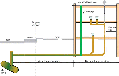
As sewer infrastructure deteriorates, managers are challenged to maintain an acceptable level of service provision, given the available budget. This has led to the development of proactive management strategies where work is prioritised based on both the estimated sewer condition and the consequences of a failure (Le Gauffre et al., 2007; Wirahadikusumah, Abraham, & Iseley, 2001). Although these proactive strategies are increasingly applied to main sewers, the lateral sewers transporting sewage from properties to main sewers (schematised in Figure 1) are generally subject to repair only after an incident occurs. Next to being less cost-effective (Fenner, 2000), this reactive approach renders customers directly exposed to the consequences of blockage incidents. The impact of a blockage in these components is not limited to a decrease in the available discharge capacity, but may extend to tangible flood damage to properties (Ten Veldhuis, Clemens, & van Gelder, 2011) and potential health risks (de Man et al., 2014). As such, a blockage directly affects the serviceability of a sewer system.

Figure 1. Schematisation of a lateral house connection.

Recently, lateral house connections have received more attention. For example, in the UK, the responsibility for the lateral connections has been transferred to the public sewer network (HMG, 2011). In Germany, the DIN 1986-30 (2012) requires evidence of the water tightness of existing lateral house connections. Arthur, Crow, Pedezert, and Karikas (2009) analysed a complaint database and reported an increased blockage likelihood for pipe diameters smaller than 0.225 m. These findings are in line with Post, Pothof, Ten Veldhuis, Langeveld, and Clemens (2015), who found blockage rates of lateral house connections to be two orders of magnitude greater than rates for main sewers. The authors suggested these results reflect differences in physical properties and governing flow regimes. Moving away from reactive strategies requires information on the condition of these components, which is typically not available.

Modelling the condition of sewers is considered difficult, due to the extensive amount of factors influencing the complex deterioration processes (e.g. Ana and Bauwens (2010) and Rajani and Kleiner (2001)). Therefore, Rodríguez, McIntyre, Díaz-Granados, and Maksimović (2012) opted for a statistical approach to analyse blockage events. Several studies have been devoted to deterioration modelling of main sewers through empirical equations based on physical properties such as pipe material, diameter, slope, age and depth (see e.g. Ariaratnam, El-Assaly, and Yang (2001) Baik, Jeong, and Abraham (2006), and Le Gat (2008)). However, data on these properties are generally lacking for lateral house connections, limiting the factors available to explain differences in observed blockage incidences. The effect of missing factors are, however, present in the spatial patterns of observed blockages. By incorporating these spatial patterns in the modelling approach, the effect of missing factors is mitigated. Hence, this paper describes a statistical approach that takes into account the spatial variation of lateral house connection blockage data to direct inspection and rehabilitation activities by identifying parts of the system with significant higher blockage likelihood. In addition, the identification of external factors discriminating blocked lateral house connections from the stock of non-blocked lateral house connections may help to identify blockage-prone areas in catchments where blockage data have not yet been collected. This study includes two examples where the described modelling approach is applied to blockage databases from two cities.

2. Methods

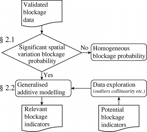
Call data from a sewer drainage company specialised in resolving small diameter (≤200 mm) sewer blockages were analysed by following the procedure described in Figure 2. The procedure first removes inconsistencies and errors from the data-set. This step removes duplicate calls for the same event, registration errors, events due to in-house sewer defects and cases where no defect is established. Subsequently, the presence of spatial variation in observed blockage incidences is evaluated to determine whether all areas experience the same blockage likelihood. A non-parametric test for spatial variation is discussed in Section 2.1. The occurrence of significant spatial variation confirms that not all lateral house connections experience the same blockage likelihood and motivates the identification of factors that explain this spatial variation. Section 2.2 discusses a semi-parametric regression model which is able to incorporate relevant factors that indicate the presence of a blockage. Since data on the physical characteristics of lateral house connections are limited, this model includes an extra term to improve the performance by accounting for the spatial variation caused by missing factors.

Figure 2. Procedure for analysis of spatial blockage data. References to the corresponding Sections where the methods are elaborated have been added.

2.1. Non-parametric testing for the presence of spatial variation

Exploring the spatial variability of blockages in a region requires a mixed database with both residential properties that reported one or more blockages λ₁ (event data) and residential properties that did not experience any blockage λ₀ (non-event data). This is necessary to normalise observed blockage rates with the number of residential properties. The blockage intensity is the ratio between events and non-events and is given by:(1)

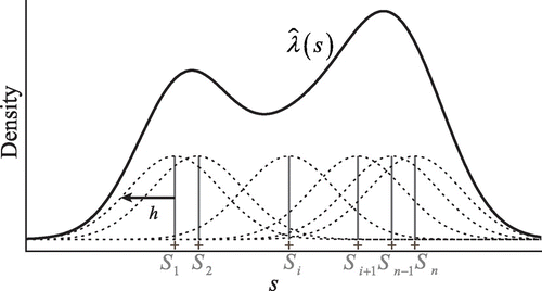
Direct analysis of the ratio between events and non-events is impracticable, as both data are discrete and do not occur at the same location. Kelsall and Diggle (1995b) computed the bivariate kernel density function to create a continuous two-dimensional surface from discrete event data with known spatial coordinates. Figure 3 illustrates this principle by showing the cross section of a kernel density function. Kernel density estimation has been applied in the field of urban drainage for the spatial analysis of flood event data (e.g. Caradot, Granger, Chapgier, Cherqui, and Chocat (2011) and Cherqui, Belmeziti, Granger, Sourdril, and Le Gauffre (2015)).

Figure 3. Example of the cross section of a bivariate kernel density function at coordinates s, given by the sum of n kernels at coordinates S₁, S_i, … S_n coordinates and bandwidth h.

The bivariate kernel density estimate for coordinates s on a regular two-dimensional grid, given a sample of n₁ blockages having coordinates S₁, S_i, … S_n, is given by:(2)

where κ is the Gaussian kernel function. The smoothing bandwidth h (i.e. a measure of standard deviation) controls how the density is spread around the point of interest. It is considered a critical parameter, as its value can have a large effect on the accuracy of the estimator (Silverman, 1986; Wand & Jones, 1995). Choosing an inappropriate bandwidth can result in over-smoothed estimates that mask characteristics of the underlying blockage data. The likelihood based cross validation principle suggested by Habbema, Hermans, and Silverman (1974) and Duin (1976) is given by:(3)

As implemented in the Spatstat library, (Baddeley & Turner, 2005) R statistical programming software (Team R Core, 2014) was used to determine the optimum bandwidth. Testing of the null hypothesis of a constant blockage intensity was performed by means of a Monte Carlo simulation, using the statistic (Bivand, Pebesma, Gomez-Rubio, & Pebesma, 2008):(4)

where n₀ is the number of non-events, c is the grid cell size and p the number of grid cells. This test statistic is computed k times, where each simulation consists of the kernel density estimation of randomly relabelled events and non-events. These simulations form the null hypothesis of constant blockage intensity for the region (Kelsall & Diggle, 1995a). The extent to which the observed blockage patterns match these simulations determines whether the null hypothesis is accepted. This is represented in the p-value, which is estimated by computing the proportion of simulations where the test statistic exceeds that of the observed blockage data. When the p-value is not consistent with the hypothesis of a constant blockage intensity for the system, there is a significant difference in the lateral house connection blockage likelihood throughout the system under observation.

2.2. Generalised additive modelling

This section introduces the regression method used for the identification of factors that distinguish properties with lateral connection blockages from the rest of the property stock. A generalised additive model (GAM) (Hastie & Tibshirani, 1986) is a semiparametric model that extends the generalised linear model (GLM), which itself is a generalisation of the well-known linear model. GLMs extend the linear modelling framework by relaxing the assumption that observations come from a normal distribution. This is essential for the analysis of blockage count data, which are characterised by non-negative integer values. These properties make the Poisson distribution particularly suited as sampling distribution (Fox, 2008).

When data on certain relevant factors are unavailable, the models ability to explain spatial variation in blockage incidences decreases. Next to a reduction in model performance, the remaining unexplained spatial variation may elicit overestimation of the statistical significance of factors in the model (Cressie, 1993). A GAM extends the GLM with an additional non-parametric smoothing term. This non-linear smoothing function f attempts to capture the excess spatial variation caused by these inadvertently omitted factors by incorporating the spatial structure of the blockage data in terms of x- and y-coordinates. The general form of this model can be expressed as:(5)

where the natural logarithm links the sampling distribution of the observations to the linear predictor. Applying the natural logarithm as a link function ensures that the fitted values are positive, regardless of the estimated regression weights.

Moreover, β refers to the estimated regression weight assigned to each of the j factors u (see Table 2), that are expected to be correlated to the occurrence of a blockage. Maximum likelihood estimates for the regression weights were obtained by the method of penalised iteratively reweighted least squares (Wood, 2000) as implemented in the R library MGCV (Wood, 2006). Penalised regression splines were used as a smoothing function. A spline consists of multiple consecutive fitted polynomials that form a smooth connection at the end of each subdomain. To prevent over-smoothing, the optimum amount of smoothing was determined by means of cross validation.

2.2.1. Bootstrapping

The technique described in this section faces two potential challenges:

•	Blockage databases are generally imbalanced in the sense that there is an abundance of non-events, i.e. properties with no blockage, which may result in biased regression estimates and standard errors (Zuur, Ieno, Walker, Saveliev, & Smith, 2009).
•	Estimated p-values for GAMs are known to be less accurate (Keele, 2008).

Bootstrapping is a nonparametric resampling technique that is able to provide a solution to both issues. By resampling the blockage data as input for the GAM, the statistical uncertainty of the estimated regression estimates is quantified without making an assumption about the underlying distribution of each weight β. In addition, bootstrapping can counter the imbalance effect using a technique from the field of machine learning known as oversampling (e.g. Osawa, Mitsuhashi, Uematsu, and Ushimaru (2011) and Radivojac, Chawla, Dunker, and Obradovic (2004)). This method assigns different sampling probabilities to events and non-events to obtain a balanced bootstrap ensemble that is not hindered by the effect of non-event abundance.

2.2.2. Model performance

The receiver operating characteristic (ROC) curve summarises model performance by graphically presenting the trade-off between correctly classified blockages and misclassified non-events. The area under the curve (AUC) is a commonly used performance measure for the ROC curve (Bradley, 1997). This measure can be interpreted as the probability that a randomly chosen blocked lateral house connection is rated as more likely to be blocked than a randomly chosen property that did not experience a blockage. A value of 1.0 means that the model is capable of fully discriminating blocked connections from the rest of the property stock, while the baseline of 0.5 represents an accuracy equal to a completely random predictor. This measure of model performance was computed using an independent validation set, obtained from blockage data that was left out of the bootstrap sample.

3. Materials

The data introduced in this chapter serve as a practical application of the methods from Chapter 2. A blockage database originating from a commercial sewer maintenance company that specialises in resolving small diameter (<200 mm) sewer blockages was interrogated. This company serves mainly businesses, private property owners and housing associations. Close to 2.3 million cases collected over 10 years were available in this blockage database. Examination of these data provided no apparent evidence of increasing or decreasing blockage rates in this period, indicating the assumption of a constant rate to be justified. Blockage data pertaining to the cities of Rotterdam and The Hague were selected from the database as case examples.

As lateral connections are (partly) located on privately owned ground, authorities in the Netherlands generally require residents to proof that a defect is in the municipal part of the sewer before they cover the costs. Therefore, this type of database has a good coverage of events on both parts. In addition, it is not uncommon that the cleaning methods used by commercial sewer companies also resolve blockages located in the municipal part of the lateral connection. As a result, it is likely that municipal call databases underestimate the true number of blockages. For instance, the number of calls received by the commercial sewer company in The Hague is with 1.28 per 100 houses per year a factor 7 greater than the municipality (0.18 calls per 100 houses per year (Gemeente Den Haag, 2011)).

3.1. Subsetting data

With a combined population of 1.1 million inhabitants (Statistics Netherlands, 2015) the cities of Rotterdam and The Hague are the second and third largest in the Netherlands. Table 1 presents a summary of urban drainage system characteristics for the two cases.

Table 1. Characteristics of Rotterdam and The Hague city examples.

Characteristics	The Hague		Rotterdam
Number of residential properties	239,145	(–)	297,740	(–)
Number of inhabitants served	495,085	(–)	610,385	(–)
Ground level variation	1–12	m	0–8	m
Number of lateral house connections	234,000	(–)	297,000	(–)
Construction year sewer	1890–2016	(–)	1920–2016	(–)
Total length foul sewers	246	km	152	km
Total length combined sewers	845	km	1779	km

A subset of blockage data from housing associations where the commercial sewer maintenance company was the sole service provider was taken. These housing associations were responsible for maintenance and repairs. Selection of housing associations with a service contract offers the following benefits:

•	A complete coverage of all blockage events, since the maintenance company is the sole service provider.
•	An overview of the property stock that did not experience blockages (non-events) in the period of observation.

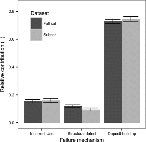
The housing associations in the subset represent 26–30% of the total property stock in Rotterdam and The Hague respectively. In addition, any high-rise buildings were discarded from the analysis, to ensure that each lateral connection serves one address exclusively. Figure 4 presents the relative contribution of different failure mechanisms for both the full data-set and the analysed set containing data on 27,144 lateral connections. Similarity of the distributions indicates that the subset is representative for the database.

Figure 4. Distribution of the observed failure mechanisms: incorrect use (e.g. sanitary towels, kitchen waste etc.), structural defect, deposit build up for both the full data-set and the analysed subset. Error bars represent 95% bootstrap confidence intervals.

3.2. Factors that indicate an increase in blockage likelihood

Lateral house connections are characterised by diameters ranging from 117 to 200 mm and gradients varying between 1:50 and 1:200 (Nederlands Normalisatie Instituut, 2011). Factors that may indicate an increased blockage propensity of lateral house connections were identified in Post et al. (2015) and through interviews with sewer managers. Detailed data on the physical characteristics of these connections are, however, not available. Instead, factors that indicate an increase in the likelihood of a blockage were divided in three groups: physical properties of the main sewer, external factors and socio-economic factors. An overview of the factors included in the modelling approach is given in Table 2.

Table 2. Factors that may indicate an increase in the likelihood of a blockage.

Factor	Type	Availability	Unit	Range
Construction year sewer	Property main sewer	Both	(year)	1900–2002
Sewer Diameter	Property main sewer	Both	(mm)	150–1000
Sewer pipe material	Property main sewer	Rotterdam	–	Concrete/plastic/vitrified clay
System type	Property main sewer	Both	–	Combined/separate
Construction year building	External	Both	(year)	1900–2002
Distance building to main sewer	External	Both	(m)	1.3–45
Private front garden	External	The Hague	–	Yes/no
Third party work activities	External	The Hague	–	Yes/no
Road state	External	Rotterdam	–	Acceptable/replacement planned
Settlement rate	External	Rotterdam	(mm/year)	1.0–6.5
Neighbourhood mean income	Socio-economic	Both	(euro∙10^–³/year)	7.70–24.20
Neighbourhood proportion non-autochthonous	Socio-economic	Both	–	[0–1]

Both cities are being served by predominately combined sewer systems constructed after 1940. They differ with respect to the soil characteristics and management policies concerning lateral house connections. The former refers to the continuous settlement of sewers in Rotterdam due to the presence of peat and clay soil, while The Hague is characterised by mainly sandy soils (Zagwijn, Beets, Van den Berg, Montfrans, & Van Rooijen, 1985). Previous research by Dirksen, Baars, Langeveld, and Clemens (2012) has shown that settlement has a substantial impact on sewer system performance. Furthermore, while in Rotterdam the homeowner is responsible for the entire connection, The Hague municipality takes responsibility for lateral connections up to the property boundary. This means that in the absence of a private front garden, the responsibility for a lateral house connection in The Hague lies completely with the authorities. To quantify the effect of these different policies, the presence of a private front garden is included as an external factor. The distance from the property to the main sewer is used as an estimate for the length of the lateral connection.

Data on the state of the road are potentially valuable indicators for sewer blockages, as both have several common failure mechanisms (e.g. traffic load) (Davies, Clarke, Whiter, & Cunningham, 2001). In addition, these infrastructures may have interaction, as the (partial) collapse of a sewer can affect the stability of the road. Furthermore, underground infrastructure activities by a third party may damage lateral connections, affecting the operational performance of these assets. Socio-economic factors represent differences in lifestyle, which may affect the composition of domestic wastewater (Ashley, Bertrand-Krajewski, Hvitved-Jacobsen, & Verbanck, 2004). This does not only extend to differences in (sanitary) item disposal habits (Friedler, Brown, & Butler, 1996), but may also reflect in food preparation habits that increase the fat, oil and grease (FOG) stock available for accumulation in sewers (Shin, Han, & Hwang, 2015).

4. Results and discussion

This chapter presents the results of the procedure introduced in Chapter 2 applied to two test examples. First, mapping of the blockage intensity surface and the corresponding results of the Monte Carlo simulation are presented in Section 4.1. Subsequently, Section 4.2 identifies factors that may indicate an increase in the blockage likelihood by means of the bootstrapped GAM. The remainder of this chapter discusses the performance of this model and the implications for management strategies.

4.1. Significance of the spatial variation

4.1.1. Bandwidth of the kernel function

Both the properties that reported at least one blockage and properties that reported no blockage were used to estimate a joint smoothing bandwidth for the kernel density function. Figure 5 shows the cross-validated likelihood function and the values for the bandwidth that minimise these function. Bandwidth values for both test examples are of a similar order of magnitude. These values represent the standard deviation of the Gaussian kernel and are a measure of the distance at which individual blockages still contribute to the kernel density estimate at a given point in space. The extent to which the derived bandwidth values are transferable to other cases depends on the characteristic spatial scale of the blockage patterns.

Figure 5. Shape of the likelihood based cross validation (CV) function 2–3 for the bandwidth h of the kernel density function 2–2. Vertical grey lines show the optimum values.

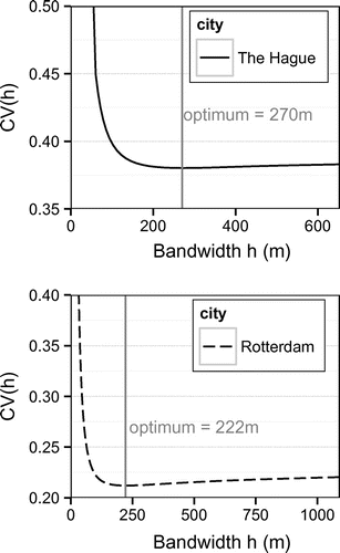
In both cases, the likelihood function is less sensitive to larger values for the bandwidth. Arguably, adopting the relative small estimated bandwidth in this flat region is supported by the fact that larger values for the bandwidth may cause over-smoothing that hides features in the underlying data.

4.1.2. Estimated p-value

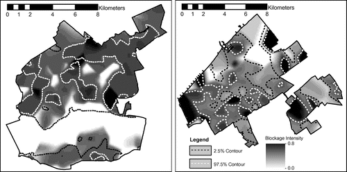
Results for the significance test of a spatially constant blockage intensity for the entire system yield significant p-values for both Rotterdam (p = 0.001) and The Hague (p = 0.004), based on 999 simulations. These results provide evidence of substantial spatial variation in the intensity of lateral house connection blockages. Statistical significance of local peaks are visualised in Figure 6 by means of contours of the 0.975 and 0.025 p-values derived from the simulations. This figure shows several hotspots experiencing significantly high blockage intensities. Interestingly, some areas with high estimated blockage intensities were found to be outside the p-value surfaces, indicating non-significance. Detailed inspection of the underlying blockage data revealed those areas to have a low building density, resulting in an estimate of the local blockage intensity that is inflated when the denominator of Equation (1(1) ) approaches zero. This demonstrates the added value of the Monte Carlo test approach, as this method is insensitive to regions with a low data density where the occurrence of a single blockage event has a profound impact on the estimated intensity.

Figure 6. Kernel ratio of the intensity of blockages for Rotterdam (left panel) and The Hague (right panel). Dark colours denote regions with a high blockage intensity. White dashed lines and black dashed lines indicate the 97.5% and 2.5% Monte Carlo simulation contours respectively. P-values for both Rotterdam (0.001) and The Hague (0.004) provided evidence to reject the hypothesis of a constant blockage intensity for the city.

4.2. Factors explaining the spatial variation in observed blockage incidences

Rejection of the hypothesis of a constant blockage intensity for both cities motivated application of the bootstrapped GAM approach discussed in Section 2.2. This regression model quantified the contribution of the explanatory factors specified in Section 3.2 to the observed blockage incidences. The extra nonparametric smoothing term was added to improve model performance by accounting for missing spatially varying factors. All continuous factors were standardised to obtain the same unit for every regression estimate β.

4.2.1. Data exploration

Exploration of the data revealed a high Pearson correlation between the factors ‘neighbourhood mean income’ and ‘neighbourhood proportion non-autochthonous’ for the cities of The Hague (−0.88) and Rotterdam (−0.67). This correlation can likely be attributed to differences in the level of education (Lautenbach & Otten, 2007). High correlations between factors may inflate model parameter standard errors (Zuur, Ieno, & Elphick, 2010), making valid inferences on relevant factors more difficult. Also taking into account the moderate correlation with other factors, it was decided to drop the latter factor (‘neighbourhood proportion non-autochthonous’) from the set.

4.2.2. Structure of the linear predictor

A distribution of weights β for each factor based on 50,000 bootstrap samples was derived from the GAM. Subsequently, confidence intervals containing the true value of the regression weights β with probability 0.95 were computed. The sample size showed to be sufficient for the distributions of regression weights to converge to stable values for the 95% confidence intervals. These intervals were adjusted for bias and skewness (Efron, 1987) to obtain accurate estimates. When the computed 95% interval contains zero for a given factor, it is concluded that the factor is not significantly different from zero at the 5% level. The final structure of the linear predictor in Equation (5(5) ) consists of all the significant factors.

4.2.2.1. Case I: The Hague

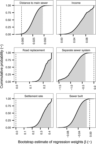
Figure 7 depicts the empirical cumulative distribution of all the regression weights β for The Hague that were found to be significant. A cumulative probability of 0.50 is equivalent to the median. From the median values of the weights β (see also Table 3), it can be concluded that the year of building construction was the dominant continuous factor discriminating lateral house connections that experience blockages from the rest of the stock (β_{property build} = −0.215). Distributions of the weights β for both categorical factors are in the same order of magnitude.

Figure 7. Empirical cumulative distribution function of the standardised regression weights β for each factor for The Hague that is significantly different from 0, based on 50,000 bootstrap samples. The 95% confidence interval is depicted by the grey area. Factors are considered significantly different from zero, when the dashed vertical line at β = 0 is not contained within the 95% confidence interval.

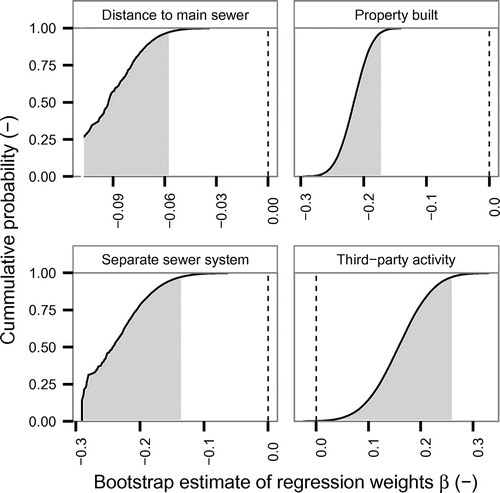
Table 3. Median estimate of the standardised regression weights β for each factor for The Hague that is significantly different from 0. The 95% confidence intervals are in parentheses.

Factor	Median	95% confidence interval
Third-party activities	0.158	[0.051, 0.262]
Separate sewer system	−0.242	[–0.290, –0.134]
Distance to main sewer	−0.093	[–0.108, –0.057]
Property built	−0.215	[–0.262, –0.170]

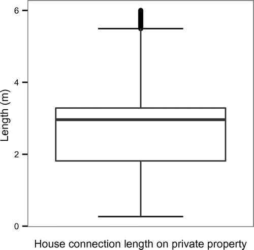
Although ‘construction year of the main sewer’ was found to be significant, this factor was dropped from the linear predictor since analysis of the bootstrap estimates revealed collinearity with ‘construction year of the property’ and to some extent with the factor ‘system type’ (see Figure 8). It seems that the presence of a garden has no effect on the blockage likelihood. This implies that the privately owned part of a lateral connection is not more susceptible to blockages than the municipal part, even though municipal policy stipulates that the municipal part should be replaced when the main sewer rehabilitation projects are initiated. On the other hand, Figure 9 shows this private part to be rather small (e.g. 30% of all gardens has a length ≤2 m), potentially obscuring any effect.

Figure 8. Correlation matrix of the regression weights β for each significant factor for The Hague, based on 50,000 bootstrap samples. Triangles indicate the strength and direction of the correlation.

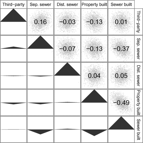
Figure 9. Boxplot of the garden lengths, used to approximate the length of the lateral house connection on private ground.

4.2.2.2. Case II: Rotterdam

The empirical cumulative distribution of the weights derived for Rotterdam is depicted in Figure 10. In comparison to example of The Hague, more factors were found to be significant. Both examples show evidence of a positive relation between age and the blockage likelihood. This might be attributed to the material use and joining methods in different time periods (Lillywhite & Webster, 1979). In addition, the time since construction can be an indicator of deterioration (e.g. Davies et al. (2001) and Marlow, Boulaire, Beale, Grundy, and Moglia (2010)). The negative weights β associated with separate sewer systems demonstrate that combined lateral connections are more prone to blockages. Arthur et al. (2009) arrived at similar findings for a sewer system in the UK.

Figure 10. Empirical cumulative distribution function of the standardised regression weights β for each factor for Rotterdam that is significantly different from 0, based on 50,000 bootstrap samples. The 95% confidence interval is depicted by the grey area. Factors are considered significantly different from zero, when the dashed vertical line at β = 0 is not contained within the 95% confidence interval.

Ground settlement was found to be the dominant continuous factor for Rotterdam (β_{ground settlement} = 0.337 according to Table 4). Sewer settlement is a common phenomenon in delta build cities. It can lead to differential settlement in combination with pile-founded buildings. These relative movements may result in deterioration such as disconnecting joints or fractures (DeSilva et al., 2005; Dirksen, 2013). Furthermore, the formation of sags due to ground settlement is conducive to the accumulation of FOG deposits (Lillywhite & Webster, 1979). The model provides evidence of a relation between the observed condition of the road and the lateral house connection blockage propensity. This leads to the hypothesis that either the condition of the road is influenced by the structural state of the underlying house connections, or both infrastructures are affected by similar latent factors.

Table 4. Median estimate of the standardised regression weights β for each factor for Rotterdam that is significantly different from 0. The 95% confidence intervals are in parentheses.

Factor	Median	95% confidence interval
Separate sewer system	−0.867	[–1.531, –0.352]
Distance to main sewer	0.026	[0.003, 0.048]
Sewer built	−0.046	[–0.083, –0.009]
Income	0.068	[0.022, 0.106]
Settlement rate	0.337	[0.217, 0.436]
Road replacement	0.213	[0.155, 0.261]

4.2.3. Improving model performance by adding a spatial smoothing function

The modelling approach adopted in this study extends a deterioration model, based on explanatory factors, with an extra term that captures any remaining spatial variation in blockage incidences. A likelihood ratio test was performed to determine whether the addition of the smoothing function f in Equation (5(5) ) resulted in a significant performance improvement. For both examples, p-values <0.001 were found, clearly favouring the models with an added smoothing function. This demonstrates that the model is capable of accounting for some of the spatial variation caused by factors (e.g. material, slope, structural defects) for which no data were available.

4.3. Classification accuracy of the model

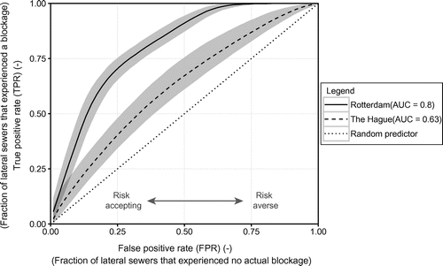
The ROC curves presented in Figure 11 present the trade-off between the proportion of correctly classified blockage events (true positive rate) and the proportion of incorrectly classified non-events (false positive rate). Clearly the modelling approach performs better for the Rotterdam example (AUC = 0.80), with classification accuracies for The Hague (AUC = 0.62) being only slightly better than a random predictor (AUC = 0.50). This may be partly attributed to the difference in data availability. For instance, ‘ground settlement rate’ is an important factor for Rotterdam, that is absent for The Hague.

Figure 11. Receiver operating characteristic (ROC) curves for both The Hague and Rotterdam, illustrating the trade-off between the true positive rate and the false positive rate. Grey areas correspond to the 95% confidence interval. The Area Under the Curve (AUC) is a measure of the overall model performance.

In terms of asset management, Figure 11 illustrates the amount of required investments on (in)correctly classified lateral house connections vs. system performance gain by preventing blockage events. For instance, Figure 11 shows that when the objective is to rehabilitate 75% of all lateral house connections in Rotterdam that experienced a blockage, 30% of all the incorrectly classified lateral house connections that did not experience a blockage will also be rehabilitated. Due to the poor model performance for The Hague, investments are less cost-effective; considerably more investments in incorrectly classified (60%) are needed to cover 75% of all lateral house connections that experienced a blockage. The left quadrant of Figure 11 is more risk-accepting, corresponding to less proactive activities, while requiring more reactive activities. The right quadrant is more risk-averse and is aimed at reducing reactive activities by proactively improving the condition of lateral house connections. Consequently, this figure can guide the optimisation of inspection and rehabilitation strategies based on the modelling approach discussed in this study. For example, the prioritisation of inspection activities when the ownership of lateral house connections is taken over by the water authorities or the rehabilitation of lateral house connections in conjunction with main sewer projects.

5. Conclusions

This study describes a procedure to analyse the spatial variation of lateral house connection blockages to identify parts of the system where proactive management strategies are most effective. The main scientific contribution of this procedure is the inclusion of a spatial smoother in deterioration modelling to improve model performance. Blockage data from commercial sewer maintenance companies are potentially valuable sources of information that can complement municipal databases to quantify the overall level of service provided by sewer infrastructure. For two cities, Monte Carlo simulations on data from such a company revealed a significant spatial variation in the blockage likelihood. Subsequently, the bootstrapped GAM was able to identify factors that distinguish blocked laterals from the remaining stock.

Age seems to be a relevant deterioration indicator for the two examples discussed. In addition, lateral house connections draining to separate systems experience lower blockage incidence compared to combined systems. The relationship between the blockage propensity and third-party (planned) activities indicates the presence of shared failure mechanisms or the interaction between different types of infrastructures. Furthermore, addition of a spatial smoother function significantly improved model predictions. This demonstrates the added value of the applied modelling approach, as it is able to mitigate the effect of unknown, but relevant, factors that are missing in the linear predictor of the model.

Analysis of the ROC curves provide key information for decision-making, by taking into account the GAM performance in assessing the trade-off between costs and benefits in terms of blocked lateral house connections. This supports the formulation of management strategies that balance serviceability vs. investments required for inspection and rehabilitation. In the total absence of data on relevant factors that may indicate increased blockage likelihood, investigation of the Monte Carlo simulation results provides an overview of areas with a significant higher blockage incidence where inspection and rehabilitation activities are most effective.

List of notations
Ρ	=	blockage intensity
λ1	=	event data
λ0	=	non-event data
κ	=	Gaussian kernel
s	=	spatial grid points where the intensity is estimated
S	=	spatial coordinates lateral house connections
c	=	grid cell size
p	=	number of grid cells
h	=	smoothing bandwidth
n0	=	number of non-events
n1	=	number of events
	=	Monte Carlo test statistic
f	=	non-linear smoothing function
η	=	expected value of the dependent variable
β	=	regression weights assigned to factors u
u	=	factors in the linear predictor

Disclosure statement

No potential conflict of interest was reported by the authors.

Acknowledgements

The authors would like to extend their gratitude to Riool Reinigings Service (RRS) for providing blockage data. The research was performed within the Dutch ‘Kennisprogramma Urban Drainage’ (Knowledge Programme Urban Drainage). The involved parties are: ARCADIS, Deltares, Evides, Gemeente Almere, Gemeente Arnhem, Gemeente Breda, Gemeente ‘s-Gravenhage, Gemeentewerken Rotterdam, Gemeente Utrecht, GMB Rioleringstechniek, Grontmij, KWR Watercycle Research Institute, Royal HaskoningDHV, Stichting RIONED, STOWA, Tauw, vandervalk + degroot, Waterboard De Dommel, Waternet and Witteveen + Bos.

References

- Ana, E., & Bauwens, W. (2010). Modeling the structural deterioration of urban drainage pipes: the state-of-the-art in statistical methods. Urban Water Journal, 7, 47–59. doi:10.1080/15730620903447597
- Ariaratnam, S. T., El-Assaly, A., & Yang, Y. (2001). Assessment of infrastructure inspection needs using logistic models. Journal of Infrastructure Systems, 7, 160–165. doi:10.1061/(ASCE)1076-0342(2001)7:4(160).
- Arthur, S., Crow, H., Pedezert, L., & Karikas, N. (2009). The holistic prioritisation of proactive sewer maintenance. Water Science & Technology, 59, 1385–1396. doi:10.2166/wst.2009.134
- Ashley, R. M., Bertrand-Krajewski, J. L., Hvitved-Jacobsen, T., & Verbanck, M. (2004). Solids in sewers. London, UK: IWA.
- Baddeley, A. J., & Turner, R. (2005). Spatstat: An R package for analyzing spatial point pattens. Journal of Statistical Software, 55(11), 1–43. doi:http://dx.doi.org/10.18637/jss.v012.i06
- Baik, H., Jeong, H., & Abraham, D. M. (2006). Estimating transition probabilities in markov chain-based deterioration models for management of wastewater systems. Journal of Water Resources Planning and Management, 132, 15–24. doi:10.1061/(ASCE)0733-9496(2006)132:1(15)
- Bivand, R. S., Pebesma, E.J., Gomez-Rubio, V., & Pebesma, E. J. (2008). Applied spatial data analysis with R. New York, NY: Springer.
- Bradley, A. P. (1997). The use of the area under the ROC curve in the evaluation of machine learning algorithms. Pattern Recognition, 30, 1145–1159. doi:10.1016/S0031-3203(96)00142-2
- Caradot, N., Granger, D., Chapgier, J., Cherqui, F., & Chocat, B. (2011). Urban flood risk assessment using sewer flooding databases. Water Science & Technology, 64, 832–840. doi:10.2166/wst.2011.611
- Cherqui, F., Belmeziti, A., Granger, D., Sourdril, A., & Le Gauffre, P. (2015). Assessing urban potential flooding risk and identifying effective risk-reduction measures. Science of The Total Environment, 514, 418–425. doi:10.1016/j.scitotenv.2015.02.027
- Cressie, N. (1993). Statistics for spatial data. New York, NY: Wiley.
- Davies, J. P., Clarke, B. A., Whiter, J. T., & Cunningham, R. J. (2001). Factors influencing the structural deterioration and collapse of rigid sewer pipes. Urban Water, 3, 73–89. doi:10.1016/S1462-0758(01)00017-6
- de Man, H., van den Berg, H. H. J. L., Leenen, E. J. T. M., Schijven, J. F., Schets, F. M., van der Vliet, J. C., van Knapen, F., & de Roda Husman, A. M. (2014). Quantitative assessment of infection risk from exposure to waterborne pathogens in urban floodwater. Water Research, 48, 90–99. doi:10.1016/j.watres.2013.09.022
- DeSilva, D., Burn, S., Tjandraatmadja, G., Moglia, M., Davis, P., Wolf, L., Held, I., Vollertsen, J., Williams, W., & Hafskjold, L. (2005). Sustainable management of leakage from wastewater pipelines. Water Science and Technology, 52, 189–198.
- DIN 1986-30. (2012). Drainage systems on private ground - Part 30: Maintenance. Berlin: DIN Standards Committee Water Practice.
- Dirksen, J. (2013). Monitoring ground settlement to guide sewer asset management. Delft: TU Delft, Delft University of Technology.
- Dirksen, J., Baars, E., Langeveld, J., & Clemens, F. (2012). Settlement as a driver for sewer rehabilitation. Water Science and Technology, 66, 1534. doi:10.2166/wst.2012.347
- Duin, R. P. W. (1976). On the choice of smoothing parameters for Parzen estimators of probability density functions. IEEE Transactions on Computers, 11, 1175–1179. doi:http://dx.doi.org/10.1109/TC.1976.1674577
- Efron, B. (1987). Better bootstrap confidence intervals. Journal of the American Statistical Association, 82, 171–185. doi:10.1080/01621459.1987.10478410
- Fenner, R. A. (2000). Approaches to sewer maintenance: A review. Urban Water, 2, 343–356. doi:10.1016/S1462-0758(00)00065-0
- Fox, J. (2008). Applied regression analysis and generalized linear models (2nd ed.). Thousand Oaks, CA: Sage.
- Friedler, E., Brown, D. M., & Butler, D. (1996). A study of WC derived sewer solids. Water Science and Technology, 33, 17–24. doi:10.1016/0273-1223(96)00365-4
- Den Haag, G. (2011). Gemeentelijk Rioleringsplan Den Haag 2011–2015: Goed riool, gezonde leefomgeving. The Hague: Municipality of The Hague, Netherlands.
- Habbema, J. D. F., Hermans, J., & Silverman, B. W. (1974). A stepwise discriminant analysis program using density estimetion. Paper presented at the Compstat, Wien, Austria.
- Hastie, T., & Tibshirani, R. (1986). Generalized additive models. Statistical Science, 297–310.10.1214/ss/1177013604
- HMG (2011). The water industry (schemes for adoption of private sewers) regulations 2011. London, UK: The Stationery Office.
- Keele, L. J. (2008). Semiparametric regression for the social sciences. Chichester: Wiley.
- Kelsall, J. E., & Diggle, P. J. (1995a). Kernel estimation of relative risk. Bernoulli, 1, 3–16. doi:10.2307/3318678
- Kelsall, J. E., & Diggle, P. J. (1995b). Non-parametric estimation of spatial variation in relative risk. Statistics in Medicine, 14, 2335–2342. doi:10.1002/sim.4780142106
- Lautenbach, H., & Otten, F. (2007). Inkomen allochtonen blijft achter door lage opleiding. Voorburg, Netherlands: Centraal Bureau voor de Statistiek.
- Le Gat, Y. (2008). Modelling the deterioration process of drainage pipelines. Urban Water Journal, 5, 97–106. doi:10.1080/15730620801939398
- Le Gauffre, P., Joannis, C., Vasconcelos, E., Breysse, D., Gibello, C., & Desmulliez, J. (2007). Performance indicators and multicriteria decision support for sewer asset management. Journal of Infrastructure Systems, 13, 105–114. doi:10.1061/(ASCE)1076-0342(2007)13:2(105)
- Lillywhite, M. S. T., & Webster, C. J. D. (1979). Investigations of drain blockages and their implications on design. The Public Health Engineer, 7, 53–60.
- Marlow, D. R., Boulaire, F., Beale, D. J., Grundy, C., & Moglia, M. (2010). Sewer performance reporting: Factors that influence blockages. Journal of Infrastructure Systems, 17, 42–51. doi:10.1061/(ASCE)IS.1943-555X.0000041
- Nederlands Normalisatie Instituut. (2011). Drainage system inside and outside buildings. Delft, The Netherlands: NEN 3215:2011.
- Osawa, T., Mitsuhashi, H., Uematsu, Y., & Ushimaru, A. (2011). Bagging GLM: Improved generalized linear model for the analysis of zero-inflated data. Ecological Informatics, 6, 270–275. doi:10.1016/j.ecoinf.2011.05.003
- Post, J. A. B., Pothof, I. W. M., Ten Veldhuis, J. A. E., Langeveld, J. G., & Clemens, F. H. L. R. (2015). Statistical analysis of lateral house connection failure mechanisms. Urban Water Journal, 13, 69–80. doi:10.1080/1573062X.2015.1057175
- Radivojac, P., Chawla, N. V., Dunker, A. K., & Obradovic, Z. (2004). Classification and knowledge discovery in protein databases. Journal of Biomedical Informatics, 37, 224–239. doi:10.1016/j.jbi.2004.07.008
- Rajani, B., & Kleiner, Y. (2001). Comprehensive review of structural deterioration of water mains: physically based models. Urban Water, 3, 151–164. doi:10.1016/S1462-0758(01)00032-2
- Rodríguez, J. P., McIntyre, N., Díaz-Granados, M., & Maksimović, Č. (2012). A database and model to support proactive management of sediment-related sewer blockages. Water Research, 46, 4571–4586. doi:10.1016/j.watres.2012.06.037
- Shin, H., Han, S., & Hwang, H. (2015). Analysis of the characteristics of fat, oil, and grease (FOG) deposits in sewerage systems in the case of Korea. Desalination and Water Treatment, 54, 1318–1326. doi:10.1080/19443994.2014.910141
- Silverman, B. W. (1986). Density estimation for statistics and data analysis (Vol. 26). London: CRC press.
- Statistics Netherlands. (2015). Retrieved October 2015, from http://statline.cbs.nl/
- Team R Core. (2014). R: A language and environment for statistical computing. Vienna, Austria: R Foundation for Statistical Computing.
- Ten Veldhuis, J. A. E., Clemens, F. H. L. R., & van Gelder, P. H. A. J. M. (2011). Quantitative fault tree analysis for urban water infrastructure flooding. Structure and Infrastructure Engineering, 7, 809–821. doi:10.1080/15732470902985876
- Wand, M., & Jones, M. (1995). Kernel Smoothing, Vol. 60 of Monographs on statistics and applied probability. London: Chapman and Hall.
- Wirahadikusumah, R., Abraham, D., & Iseley, T. (2001). Challenging issues in modeling deterioration of combined sewers. Journal of Infrastructure Systems, 7, 77–84. doi:10.1061/(ASCE)1076-0342(2001)7:2(77)
- Wood, S. (2006). Generalized additive models: An introduction with R. Boca Raton, FL: CRC press.
- Wood, S. N. (2000). Modelling and smoothing parameter estimation with multiple quadratic penalties. Journal of the Royal Statistical Society. Series B, Statistical Methodology, 62, 413–428, doi:10.1111/1467-9868.00240
- Zagwijn, W. H., Beets, D. J., Van den Berg, M., Montfrans, H. M., & Van Rooijen, P. (1985). Atlas van Nederland (Vol. 13). The Hague, Netherlands: Staatsuitgeverij.
- Zuur, A., Ieno, E. N., Walker, N., Saveliev, A. A., & Smith, G. M. (2009). Mixed effects models and extensions in ecology with R. New York, NY: Springer Science & Business Media.10.1007/978-0-387-87458-6
- Zuur, A. F., Ieno, E. N., & Elphick, C. S. (2010). A protocol for data exploration to avoid common statistical problems. Methods in Ecology and Evolution, 1, 3–14. doi:10.1111/j.2041-210X.2009.00001.x