Downscaling an intense precipitation event in complex terrain: the importance of high grid resolution

ABSTRACT

Floods due to intense rainfall are a major hazard to both people and infrastructure in western Norway. Here steep orography enhances precipitation and the complex terrain channels the runoff into narrow valleys and small rivers. In this study we investigate a major rainfall and flooding event in October 2014. We compare high-resolution numerical simulations with measurements from rain gauges deployed in the impacted region. Our study has two objectives: (i) to understand the dynamical processes that drove the high rainfall and (ii) the importance of high grid resolution to resolve intense rainfall in complex terrain. This is of great interest for numerical weather prediction and hydrological modelling. Our approach is to dynamically downscale the ERA-Interim reanalysis with the Weather Research and Forecasting model (WRF). We find that WRF gives a substantially better representation of precipitation both in terms of absolute values as well as spatial and temporal distributions than a coarse resolution reanalysis. The largest improvement between the WRF simulations is found when we decrease the horizontal model grid spacing from 9 km to 3 km. Only minor additional improvements are obtained when downscaling further to 1 km. We believe that this is mainly related to the orography in the study area and its representation in the model. Realistic representations of gravity waves and the seeder–feeder effect seem to play crucial roles in reproducing the precipitation distribution correctly. An analysis of associated wavelengths shows the importance of the shortest resolvable length scales. On these scales our simulations also show differences in accumulated precipitation of up to 300 mm over four days, further emphasising the need for resolving short wavelengths. Therefore, our results clearly demonstrate the need for high-resolution dynamical downscaling for extreme weather impact studies in regions with complex terrain.

Keywords:

• WRF
• resolution
• dynamical downscaling
• extreme precipitation
• flooding
• complex terrain

1. Introduction

Orographic enhancement of precipitation is a weather feature evident to anyone who has lived in the vicinity of mountains (Roe, 2005, and references therein). It explains why the coast in southwestern Norway is the wettest part of the country (Hanssen-Bauer and Førland, 2000). The annual averages exceed 3000 mm in several places, e.g. Jonshøgdi (station number 50310) with 3151 mm, but there is also large variability, e.g. Vossevangen (station number 51530) with 1280 mm (MET Norway, 2015). Orographic effects can, in addition to increasing climatological averages, be instrumental in generating extreme precipitation and associated hazards for life and property. Such a situation occurred in September 2005, when the remains of two tropical cyclones hit the west coast of Norway and the complex terrain induced strong rainfall enhancement on local scales (Stohl et al., 2008). The large rainfall amounts caused a fatal landslide close to the city of Bergen.

Flow towards a barrier leads to dynamical interactions between the air mass and the terrain. The nature of the reaction depends on a number of fundamental factors, such as barrier dimensions, wind speed and atmospheric moisture content of the approaching air mass (Miglietta and Buzzi, 2001, 2004). In cases with sufficient wind speed and weak, but positive moist static stability, the air mass ascends adiabatically over the barrier and sets of gravity waves. Upward motions are found immediate upstream of the barrier and as vertical gravity wave perturbations downstream of the mountain (Roe, 2005; Houze Jr., 2012). Microphysical processes, such as hydrometeor formation and fall out time, are important delaying factors in the precipitation formation. The delay results in a belt of enhanced precipitation shifted towards the hilltop and on the immediate lee side. The latter effect is often referred to as the spillover effect (e.g. Sinclair et al., 1997; Jiang and Smith, 2003). Depending on the wind speed and the mountain orography, the spillover effect can potentially influence the precipitation distribution 20 km to 30 km downstream, with realistic values of the microphysical time delay between 500 s and 2000 s (Smith, 2003).

Intense precipitation on smaller hills is observed even though the microphysical time scale is insufficient to produce precipitation. An explanation is found in the seeder–feeder effect first proposed by Bergeron (1949), where an overlaying seeder cloud, potentially independent of the barrier, produces ice nuclei that fall into a lower, terrain-induced feeder cloud. The result is an excess of condensation nuclei, which distinctly accelerates the coalescence processes compared to a non-seeded situation. Model results have shown a doubling in rain rates, caused by a pronounced decrease of the relevant time scales in droplet growth, when the seeder–feeder effect is implemented (Rutledge and Hobbs, 1983).

The ability of a model to reproduce local extremes is important for impact assessments and forecasting of devastating events caused by heavy precipitation, e.g. flooding and landslides. It requires a sufficiently high grid resolution, partly because the model is unable to represent wavelengths shorter than up to 10 times the grid size (Warner, 2011). However, a doubling in horizontal resolution and an accompanied reduction of the model’s time step, will lead to an increase in computational demands by a factor of . In addition, an increase in the vertical resolution, i.e. adding more model levels, will lead to a further increase in computational costs. It is therefore of great importance to find an appropriate model grid spacing, minimising computational demands, but still ensuring a simulation that reproduces weather extremes in a satisfactory manner.

Barrier width has previously been shown to have a large influence on the grid resolution requirements (Colle et al., 2005; Smith et al., 2015). Larger barriers generate gravity waves of longer wavelengths and thereby reduce the need for very high resolution in the model, whereas narrower barriers excite the atmosphere at shorter wavelengths and therefore require an increased horizontal resolution for an accurate description of the precipitation patterns. Many studies have demonstrated the added value that high-resolution regional models yield with respect to the coarse-resolution driving reanalysis or climate models in regions with complex terrain, including western Norway (Barstad et al., 2009; Heikkilä et al., 2011; Mayer et al., 2015), the western USA (Di Luca et al., 2012) and the Alps (Ban et al., 2014; Torma et al., 2015). Yet, the lower limit for when the increased resolution adds value is not yet fully clear.

One specific application which requires accurate information about the intensity and spatial distribution of precipitation is catchment hydrology under the aspect of flood risk projections (e.g. Wilson et al., 1979; Smith et al., 2014; Kay et al., 2015). Due to the lack of appropriate resolution, model simulations may describe the catchment and runoff improperly or distribute the precipitation into a wrong catchment area. As a consequence, the realism of horizontal distributions of precipitation has been shown to be a limiting factor in hydrology studies (e.g. Tramblay et al., 2013; Smith et al., 2014). Increasing the horizontal resolution generally allows for a more detailed representation of parameters relevant for runoff calculations, such as surface and soil properties and small-scale topographic features, leading to a more realistic hydrology. A number of studies have shown that a decrease of the grid spacing often improves the accuracy as one would primarily expect (e.g. Richard et al., 2007; Rögnvaldsson et al., 2007; Pieri et al., 2015; Smith et al., 2015), but there is also evidence that this is not always the case (e.g. Grubišić et al., 2005; Chan et al., 2013).

Here we study an episode in October 2014, when consecutive days with heavy rainfall caused widespread flooding in the mountainous areas of western Norway. Large amounts of precipitation over several days led to saturation of the top layers of the soil. At the same time, the mountains in the study area were lacking snow that could have absorbed and temporarily stored some of the water at higher altitudes. A combination of those factors resulted in unusually large runoff.

Our main motivation is to investigate to which degree a numerical weather prediction (NWP) model is able to reproduce the dynamical processes of an extreme rainfall event, and how sensitive the model result is to the choice of horizontal grid spacing. For this study we analysed model simulations with respect to structure and dynamics of the atmosphere to estimate the relevant spatial scales. We hypothesise that high horizontal resolution gives a better representation of the dynamical features that are the key drivers of the precipitation processes in the complex terrain.

The paper is organised as follows. In Section 2 we describe the data set and the methods used, including the model description and setup. The results are presented in Section 3 and discussed in more detail in Section 4, with emphasis on the sensitivity to model grid spacing and its effect on atmospheric dynamics.

2. Data and methods

2.1. Observational data

The observational precipitation data set consists of measurements from 43 stations operated by the Norwegian Meteorological Institute (MET Norway) and 11 rain gauges deployed in the Voss area in western Norway as part of a master’s project on fine-scale precipitation distribution in complex terrain (Pontoppidan, 2015). The instrument used in the field campaign was the tipping bucket rain gauge HOBO RG2-M (Onset, 2001), registering the time stamp of each tip corresponding to 0.2 mm of precipitation. The HOBO rain gauge is not heated and therefore limited to liquid precipitation sampling for reliable data. However, there was no occurrence of snow at any of the stations during the event under investigation here.

Rain gauge measurements are in general prone to undercatch, i.e. the imperfect collection of precipitation, due to wind speed dependent flow distortion around the gauge and additional losses such as wetting, evaporation and splashing (e.g. Sevruk et al., 2009; Habib et al., 2010; Mekonnen et al., 2015). Wetting and evaporation are most relevant during periods with low rain rates and were neglected in our case. The anticipated largest error, the wind-induced undercatch, was minimised during the field campaign by a similar shielded placement in the terrain. No further corrections on the wind speed dependency were applied. We therefore estimate the rain gauges to show a small undercatch that should, however, be of comparable magnitude for all stations.

Before and after the deployment period of the HOBO rain gauges, we performed a calibration check on each instrument, allowing for a correction of potential changes in the sensitivity of the instruments over time. A detailed description of the calibration check and correction procedure can be found in Pontoppidan (2015).

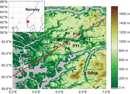
The distribution of the stations in the area is shown in Fig. 1, and the corresponding exact locations and station altitudes are given in Table 1. Hagavik (P1) and Nesttun (P2) are coastal stations at low elevation with flat terrain upstream and moderately high and steep terrain downstream. Hisdalen (P3), Dale (P4) and Kaldestad (P5) are also located at low elevations, but with steep terrain both up- and downstream. The mountainous stations, Sandfjellet (P8), Hodnaberg (P9) and Flyane (P11), are situated at higher altitudes and are also mainly surrounded by higher terrain up- and downstream. The remaining stations, Steine (P7), Dyrvedalen (P10) and Vasslii (P12), are positioned on the north side of the wider Bergen–Voss valley, in slightly upslope terrain. They all have massive barriers upstream and high terrain immediately downstream and were categorised as Valley North. Further description of the MET Norway stations is available from their website (MET Norway).

Table 1. Overview of the locations for the HOBO rain gauges (P1–P12) and the meteorological stations (denoted by their national code)

Identity	Name	Latitude	Longitude	Altitude
P1	Hagavik	60.176^◦N	5.403^◦E	48 m
P2	Nesttun	60.319^◦N	5.373^◦E	58 m
P3	Hisdalen	60.397^◦N	5.690^◦E	140 m
P4	Dale	60.590^◦N	5.829^◦E	91 m
P5	Kaldestad	60.554^◦N	6.018^◦E	521 m
P7	Steine	60.667^◦N	6.200^◦E	485 m
P8	Sandfjellet	60.607^◦N	6.212^◦E	620 m
P9	Hodnaberg	60.561^◦N	6.214^◦E	618 m
P10	Dyrvedalen	60.653^◦N	6.335^◦E	355 m
P11	Flyane	60.602^◦N	6.319^◦E	436 m
P12	Vasslii, Voss	60.645^◦N	6.445^◦E	79 m
25830	Finsevatn	60.592^◦N	7.524^◦E	1210 m
29400	Sandhaug	60.183^◦N	7.481^◦E	1250 m
46430	Røldalsfjellet	59.832^◦N	6.733^◦E	1010 m
46450	Røldal	59.830^◦N	6.824^◦E	393 m
47450	Straumøy	59.653^◦N	5.434^◦E	36 m
47500	Etne	59.665^◦N	5.966^◦E	35 m
47600	Litledal	59.664^◦N	6.066^◦E	83 m
47610	Kritle	59.636^◦N	6.087^◦E	568 m
47820	Eikemo	59.859^◦N	6.279^◦E	178 m
47890	Opstveit	59.858^◦N	6.017^◦E	38 m
48450	Husnes	59.864^◦N	5.770^◦E	13 m
48500	Rosendal	59.991^◦N	6.026^◦E	75 m
48780	Mauranger	60.132^◦N	6.331^◦E	33 m
49080	Øvre Krossdalen	60.280^◦N	6.386^◦E	342 m
49490	Ullensvang	60.319^◦N	6.654^◦E	12 m
49631	Eidfjord II	60.465^◦N	7.069^◦E	20 m
49800	Fet, Eidfjord	60.409^◦N	7.280^◦E	735 m
50070	Kvamsøy	60.358^◦N	6.275^◦E	49 m
50080	Øystese	60.379^◦N	6.193^◦E	108 m
50110	Aksneset, Kvam	60.336^◦N	6.218^◦E	13 m
50120	Skulafossen	60.275^◦N	6.039^◦E	16 m
50150	Hatlestrand	60.042^◦N	5.906^◦E	45 m
50175	Austevoll	60.017^◦N	5.206^◦E	32 m
50310	Jonshøgdi	60.389^◦N	5.964^◦E	455 m
50450	Stend	60.273^◦N	5.331^◦E	54 m
50480	Sandsli	60.292^◦N	5.280^◦E	45 m
50540	Florida	60.383^◦N	5.333^◦E	12 m
51010	Fossmark	60.521^◦N	5.724^◦E	10 m
51250	Øvstedal	60.688^◦N	5.965^◦E	316 m
51440	Evanger	60.647^◦N	6.111^◦E	17 m
51470	Bulken	60.646^◦N	6.222^◦E	328 m
51530	Vossevangen	60.625^◦N	6.426^◦E	54 m
51800	Mjølfjell	60.702^◦N	6.937^◦E	695 m
51990	Myrkdalen	60.866^◦N	6.473^◦E	700 m
52170	Eksingedal	60.803^◦N	6.147^◦E	450 m
52220	Gullbrå	60.829^◦N	6.265^◦E	579 m
52310	Modalen III	60.856^◦N	5.973^◦E	125 m
52400	Eikanger	60.623^◦N	5.381^◦E	72 m
52475	Blomvåg	60.531^◦N	4.893^◦E	30 m
52601	Haukeland	60.835^◦N	5.583^◦E	325 m
52750	Frøyset	60.846^◦N	5.211^◦E	13 m
53160	Jordalen	60.900^◦N	6.724^◦E	614 m
53530	Midtstova	60.656^◦N	7.276^◦E	1162 m

Fig. 1. Map of the experiment area with altitude from the terrain database ASTER GDEM v1 (Tachikawa et al., 2011) contoured in colours. The deployed rain gauges are colour coded and the stations P1–P12 correspond to the line colours in Fig. 5. Black squares are the stations M1–M3 referenced in the text, triangles are the remaining precipitation stations in the area operated by the Norwegian Meteorological Institute (MET Norway). The red line shows the lower edge of the cross sections analysed in Section 3.4.

2.2. Model setup

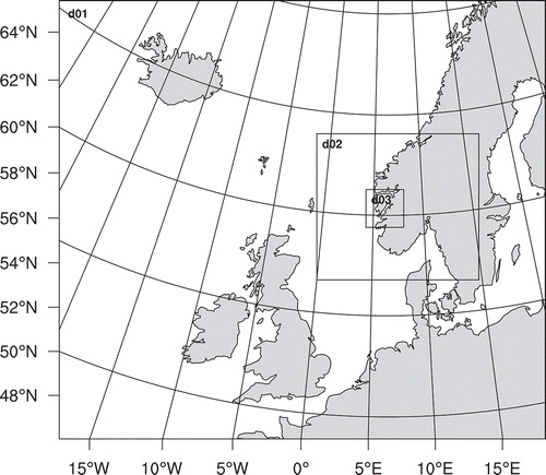
We used version 3.5.1 of the Weather Research and Forecasting model (WRF), a non-hydrostatic NWP model with terrain-following sigma coordinates (Skamarock et al., 2008). The model domain setup is shown in Fig. 2. The outer domain had 301271 grid points, with a horizontal resolution of 9 km, yielding a domain of 2709 km in the west–east direction and 2439 km in the south–north direction. The model time step in the outer domain was 45 s. The two-way nested domains, d02 and d03, had a grid resolution of 3 km and 1 km and had time steps of 15 s and 3 s, respectively. The extremely short time step of 3 s was necessary to avoid numerical instabilities in the simulation. As an additional effort to avoid instabilities, we smoothed the terrain with two passes of the smooth_desmooth option in the simulation that included all three domains. The 301271 grid points of domain d02 resulted in a domain size of 903 km813 km, while domain d03 had an extension of 211 km211 km. All three domains had 70 vertical levels with the model top at 50 hPa. The initial and boundary conditions for the outer domain were taken from the ERA-Interim reanalysis produced by the European Centre for Medium-Range Weather Forecasts (ECMWF) (Dee et al., 2011). The outer boundary conditions and sea surface temperatures were updated every 6 h during the simulation period.

Fig. 2. Model domain set up for the WRF simulations. The domains d01, d02 and d03 have horizontal grid resolutions of 9 km, 3 km and 1 km, respectively.

We used the following physical parametrisation schemes: the Kain–Fritsch cumulus scheme (Kain, 2004), Thompsons microphysics scheme (Thompson et al., 2004, 2008), the MYJ planetary boundary layer scheme (Janjić, 2000), the NOAH land surface model (Chen and Dudhia, 2001) and the Dudhia shortwave (Dudhia, 1989) and the RRTM longwave (Mlawer et al., 1997) radiation schemes. The cumulus scheme was only used in the outer 9 km domain, as the 3 km and 1 km domains are on a convection-permitting resolution. (Note that we also ran an experiment with the cumulus scheme disabled in the 9 km domain, and the results were virtually indistinguishable from the ones for the control run.)

Table 2 gives a schematic overview of the parametrisations. Various combinations of these schemes have been used in other studies (e.g. Wang et al., 2014; Weckwerth et al., 2014; Mayer et al., 2015), and this particular set of physical parameters has shown reliable results in an earlier study of precipitation in complex terrain in western Norway (Barstad and Caroletti, 2013). The sensitivity to parametrisation schemes was not the scope of this study and has not been examined closer. This has been investigated in previous studies (e.g. Rögnvaldsson et al., 2011; Efstathiou et al., 2013; Pieri et al., 2015).

Table 2. Overview of the physical parametrisation schemes used in the WRF simulations

Category of physics	Parametrisation schemes
Microphysics	Thompson (Thompson et al., 2004; 2008)
Short wave radiation	Dudhia shortwave (Dudhia, 1989)
Long wave radiation	RRTM longwave (Mlawer et al., 1997)
Planetary boundary layer	MYJ (Janjić, 2000)
Land surface model	NOAH LSM (Chen and Dudhia, 2001)
Cumulus (d01)	Kain Fritsch (Kain, 2004)
Cumulus (d02 and d03)	None

The model was initiated at 00:00 UTC on 24 October 2014, or in abbreviated form 24/00. Three different runs were performed, with two-way feedback when nests were present. One with all three domains 9 km, 3 km and 1 km, a second with the 9 km and 3 km domains and a third with just the 9 km domain. The first 30 h of the model runs were discarded as spin-up, resulting in a four-day analysis window from 25/06 to 29/06. When comparing model results with observations, we used the nearest four model grid points, weighted according to their distance to the location.

We performed different sensitivity tests to find the optimal spectral nudging settings (Von Storch et al., 2000; Omrani et al., 2012, 2015) for the simulation of precipitation during the flooding event. The best model representation of the single-location precipitation was found to be the one with the standard WRF relaxation time of 1 h and nudging wavelengths above 677 km zonally and 609 km meridionally in the outer domain only. We chose this model run for a dynamical investigation in Section 3.4. A more detailed description of the selection process based on multiple sensitivity simulations can be found in Pontoppidan (2015).

3. Extreme flooding event October 2014

3.1. Synoptic situation

End of October 2014 south-western coastal Norway was exposed to considerable amounts of precipitation, resulting in widespread flooding. One of the hardest affected areas was located along the River Vosso, and the Voss area experienced a severe flooding event on 28 October. The official stations operated by MET Norway in the area reported three-day total precipitation amounts of 249 mm for Jonshøgdi (station number 50310, M1 in Fig. 1), 133 mm for Evanger (station number 51440, M2) and 111 mm for Vossevangen (station number 51530, M3) between 26/06 and 29/06.

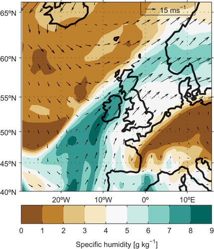
The synoptic situation a few days before the flooding event was characterised by the passage of multiple frontal systems with partly heavy precipitation. The analysis from 28/00 (Fig. 3) shows the centre of a low-pressure system over the Barents Sea and ongoing cyclogenesis over the experiment area. The frontal zones advected warm and moist air masses from the tropics towards western Norway. This is also evident in Fig. 4, which presents the specific humidity at 850 hPa from the ERA-Interim reanalysis for the same time.

Fig. 3. Surface analysis chart from UK Meteorological Office, for 28 October 2014 00 UTC. Reproduced with kind permission of the Met Office.

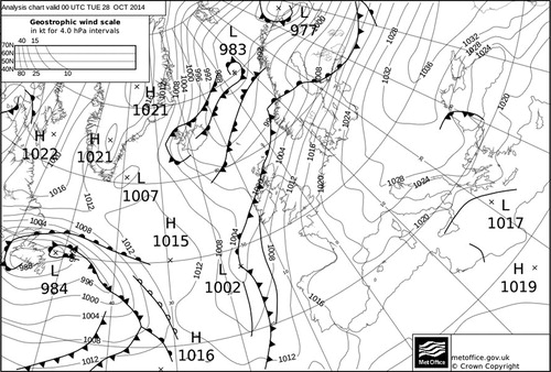
Fig. 4. Specific humidity (g kg) at 850 hPa at 00 UTC on 28 October (coloured contours) and the 850 hPa wind (arrows). Data from the ERA-Interim reanalysis.

Two days before the flooding event, on 26 October, a low-pressure system was centred NW of Norway. The associated fronts passed over western Norway and caused considerable amounts of precipitation during the day, especially around noon. A cold front passed the area at 27/00, temporarily advecting drier air and causing a relatively dry period after the frontal passage. At the same time a disturbance over Scotland developed and moved towards Norway, leaving western Norway in the warm sector of an intensifying low-pressure system with again large amounts of precipitation from 27/12 to 28/17. The associated cold front passed the Bergen area in the afternoon and the precipitation intensity behind decreased. As result of several days with more or less continuous rainfall, the flood peaked in the Voss area early evening of 28 October.

3.2. Observed and simulated precipitation

The observed precipitation during the four days prior to the flooding top is shown in Fig. 5a, with the HOBO gauges shown as coloured lines and the accumulated daily values from the MET Norway stations as black diamonds. The HOBO measurements clearly show different phases of precipitation intensity, manifested by the varying slope of the curves, related to the synoptic situation and development described above. Two distinct heavy precipitation periods are evident (all of 26 October and 27/12–28/12), separated by a dry period of about 12 h. The spatial variability among the stations was large, with an overall observed range between 340 mm at P5 and 47610 and approximately 20 mm at 29400. The span of the HOBO rain gauge values agrees with the observed precipitation range of the MET Norway stations, with P5 being amongst the stations with highest precipitation amounts and P1 in the lower part. The very low values are not captured by the HOBO gauges.

Fig. 5. The observed (a) and simulated (b) accumulated precipitation amounts during the days before the flooding event, from 25 October 06 UTC to 29 October 2014 06 UTC. The observations of the HOBO rain gauges are given as solid coloured lines and the corresponding results from the interpolated 1 km model simulations as dashed lines. Data from the MET Norway stations are indicated by the black diamonds.

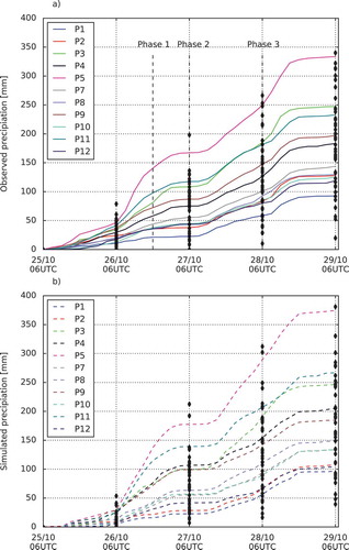
The simulated precipitation from the 1 km model run is shown in Fig. 5b. The agreement between simulated and observed precipitation is obvious. The model represented the variability, in terms of both temporal and spatial precipitation distribution, remarkably well. It showed, however, a slight tendency to underestimate the precipitation amounts during the first 24 h. The total spatial variability also seems correctly represented with the MET Norway stations spanning approximately the observed range, and both P1 and P5 close to the observed minimum and maximum values. The variability and forecast timing of the intermediate stations were also captured adequately. The two intense precipitation periods were well represented with respect to timing, and the intermediate dry period was clearly reproduced in the simulation.

3.3. Comparison of model resolutions

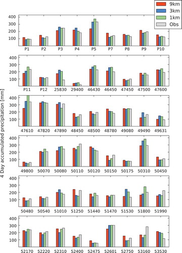
Figure 6 presents a comparison of the total four-day accumulated precipitation from 25/06 to 29/06 in the observations and simulations. For each station, the columns show the WRF simulations (9 km, 3 km and 1 km) and the observed precipitation amount. The observations were well replicated in the model simulations; one exception was station 25830, for which all the simulations overestimated the precipitation largely.

Fig. 6. Comparison of four-day accumulated precipitation from 25 October 06 UTC till 29 October 06 UTC from the WRF 9 km, 3 km and 1 km model output, using the interpolated grid point, and the observations. There is one set of bars for each station and the labels on the horizontal axis show the station id.

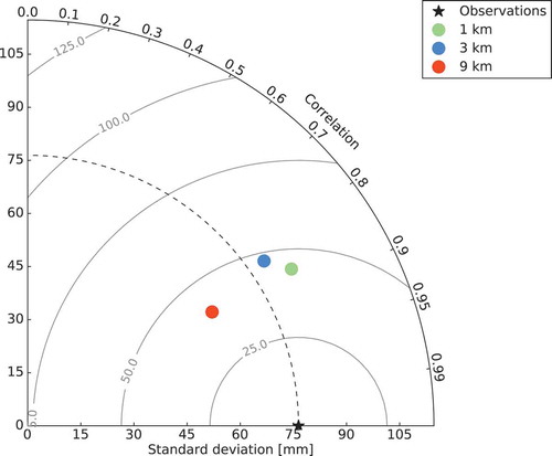
Figure 7 shows a Taylor diagram of the basic statistics for the model runs marked as coloured circles. The calculations are based on the simulated total four-day precipitation at the 54 stations. The observed standard deviation amongst the 54 stations was 76.4 mm, as marked with a black asterisk in the diagram. We notice that the coarse grid model run at 9 km underestimated the standard deviation, here representing the spatial variability amongst the stations, whereas this variability was slightly overestimated in the 3 km run, with 81.4 mm, and again slightly higher in the 1 km run, with 86.6 mm. In terms of root mean square (rms) difference, the 9 km run scored best, and for the correlation, which represents a spatial correlation (though only based on 54 stations), all runs were above 0.8. The best being the 1 km run, with the 3 km run only slightly below.

Fig. 7. A Taylor diagram with the 9 km, 3 km and 1 km simulations marked as circles and the observations marked as a black star for reference.

3.4. Dynamics

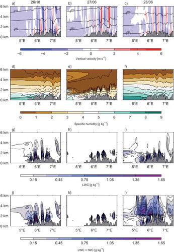
To study the underlying dynamical and physical processes, we investigated the vertical structure of the atmosphere in the model simulations. In accordance with the dominant inflow direction during the case study, we defined a SW to NE oriented cross section through the inner domain, in close vicinity to the stations P1, P3, P5, P7 and 51,470. The cross section is depicted as a red line in Fig. 1. For the following discussion, we selected the output at three model times representative for the dominant phases of the event. One during the first heavy precipitating period at 26/18, a second during the dry period at 27/06 and a third during the second heavy precipitation period at 28/06 (shown in Fig. 5a).

A series of cross sections of vertical velocity and potential temperature from the 1 km resolution run are shown in Fig. 8a–c. The air mass approached the coast as a level non-turbulent flow. When it impinged on orography higher than a few hundred meters, gravity waves formed. The gravity waves were present at all the selected times, though with slightly lower intensity at 28/06. The potential temperature showed a clear terrain-induced displacement, diminishing only slightly with altitude.

Fig. 8. Cross sections (above the red line in Fig. 1) of vertical velocities (a–c) with potential temperature contoured in black lines, specific humidity (d–f), liquid water content (g–i) and the sum of liquid and ice water content (j–l) from the 1 km resolution run, at three selected times: 26/18, 27/06 and 28/06 (in the left, middle and right column, respectively).

Figure 9a–c shows the effect of different grid resolutions on the representation of gravity waves at 28/06. The 9 km grid spacing had fewer wave cells with significantly lower intensity, and the related vertical velocities ranged between 1.0 m s and 1.7 m s. The 3 km and 1 km resolution had similar cell structures and a vertical velocity range of 3.5 m s to 3.1 m s and 5.5 m s to 3.4 m s, respectively.

Fig. 9. Cross sections (above the red line in Fig. 1) of vertical velocities (a–c), specific humidity (d–f), liquid water content (g–i) and the sum of liquid and ice water content (j–l) at time 28/06 for the 9 km, 3 km and 1 km runs (in the left, middle and right column, respectively.

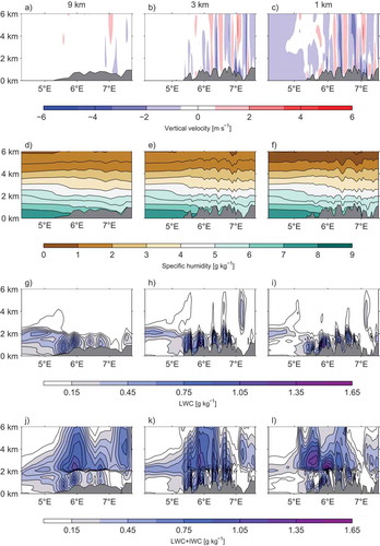
Cross sections of specific humidity at the three selected times are shown in Fig. 8d–f. The moisture content varied throughout the period, with a minimum in the dry period and a maximum at the last time shown at 28/06. Vertical displacements of drier air were evident downstream of the large mountains at all times. The major displacements caused by the large mountains were detectable throughout the lower 5 km, whereas smaller hills only caused displacement in the lower few hundred meters. The main difference in the humidity distribution between the two precipitation episodes was the considerably thicker layer of high specific humidity during the second phase (28/06), exceeding 6 g kg in the lowest 2 km of the atmosphere. During the first phase (26/18) this value only occurred in the lowest few hundred meters. The effect of the grid sizes shown in Fig. 9d–f seemed limited. The 9 km run was able to resolve the overall specific humidity at this time (28/06), and was quite similar to both the 3 km and 1 km run on a large scale. The orography did, however, affect the smaller scale specific humidity over the complex terrain.

Liquid water content (LWC) and the sum of ice water content (IWC) and LWC for the three selected times are shown in Fig. 8g–i and 8j–l. At 26/18 the LWC clearly increased over elevated orography and reached its absolute maximum over the first massive barrier crest at 5.9E. The spillover effect was detectable as the high LWC values continued downslope. Similar features, but with less intensity, were in play at the barriers further downstream. The large areal inhomogeneity in the observed precipitation during this phase was likely related to the distinct differences in LWC. Around the final time the LWC values similarly increased at the first major barrier at 5.9E, but the LWC signals were more diffuse over the remaining terrain features, distributing the precipitation more evenly. A reason for this difference may be found in Fig. 8j–l, which shows that the first precipitation phase (26/18) was nearly unaffected by ice particles having a single maxima of LWC in the vertical dimension. On the other hand, the final precipitating period (28/06) had large amounts of ice particles which created a second vertical maxima of LWC and IWC. The large and rather homogeneous distribution of ice particles aloft could be a potential seeder cloud for the cloud layers below. As a consequence of this seeding, the droplets over a large area would grow faster, fully in accordance with the observations of increased precipitation amount and decreased horizontal variability.

The effect of different horizontal resolutions on the LWC and the sum of LWC and IWC are shown in Fig. 9g–i and 9j–l, respectively. The 9 km resolution lacked a sufficient representation of the high LWC and IWC amounts in general. This resulted in a LWCIWC maximum of 0.7 g kg. The 3 km and 1 km resolution simulations had generally higher values, with maxima of 1.5 g kg and 1.8 g kg, respectively. The spillover effect is detected as increased amounts of LWC and IWC immediately downslope of hill crests in the 3 km and 1 km runs. The spillover effect seems to be absent in the 9 km run.

The horizontal distribution of accumulated model precipitation during the four-day period is presented in Fig. 10. The HOBO stations are marked on the map with circles and the MET Norway stations with squares (see Fig. 1), all filled with colours corresponding to the observed precipitation during the period. The 9 km run was unable to simulate the high precipitation amounts (Fig. 10a) and seems inadequate for further hydrological modelling. The 3 km (Fig. 10b) and 1 km (Fig. 10c) run simulated higher rainfall and higher variability, agreeing better with the observations. In the western part of the domains over the North Sea, the precipitation fields were in general homogeneous, and the absolute amounts were relatively low. The synoptic-scale forced ascent gave increased precipitation amounts closer to the coastline, and further inland the horizontal inhomogeneity was enhanced in all the simulations. For the 3 km and 1 km domain this inhomogeneity increased substantially, and small confined areas of accumulated simulated precipitation well above 600 mm can be discerned in the southern part of the area. The station P5 is located at the edge of such an area, situated at the first major terrain barrier in the flow direction. Within a radius of 5 km from this station the accumulated precipitation varied by as much as 300 mm during the four days.

Fig. 10. Accumulated precipitation (25/06–29/06 October) in part of the 9 km grid (a). The circles correspond to the HOBO stations, squares are stations from MET Norway. The inner parts of the markers show the observed accumulated precipitation amounts in the period. The other panels show the same for part of the 3 km domain in (b) and for the 1 km domain in (c).

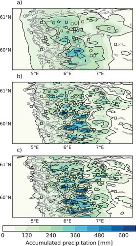
The valley to the NE of P12 and 51530 received considerably less precipitation than the steep and elevated terrain surrounding it. This area is located approximately 100 km from the coast in the SW flow direction and situated in the synoptic-scale evaporation zone in the lee of the mountainous Hamlagrø plateau. The reduced precipitation (which has been informally confirmed by locals) observed there (P12) is likely linked to the location of the station, and the enhanced precipitation amounts around it were probably caused by smaller-scale orographic features.

South in our study area, the model simulations also indicated several other precipitation hot spots. Of particular interest during the period investigated here was the area of enhanced precipitation at 60N, 6.5E. It covered large parts of the catchment of the Opo River, which was also severely affected by the flooding.

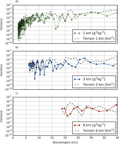
In order to identify important wavelengths, we performed a spectral analysis of the model terrain and the humidity. The 850-hPa pressure level from the 26/18 cross section of specific humidity shown in Fig. 8d–f were analysed using a discrete cosine transform (Denis et al., 2002). Figure 11a shows the variance for specific humidity and model orography for the 1 km run. Correspondingly the 3 km and 9 km simulations are shown in Fig. 11b and Fig. 11c. Since wavelengths shorter than twice the grid spacing are unresolved, the 9 km domain was unable to resolve wavelengths shorter than 18 km. For the 1 km simulation both the terrain and the specific humidity variance followed the same pattern of increasing values from the shortest resolved wavelength and upwards. The peak was reached around wavelengths of 6 km. The 3 km simulation agreed well with the 1 km run at resolved wavelengths. The similarity between the specific humidity spectra and the orography spectra, at least for the 3 km and 1 km simulations, indicates a link between the two. Similar results were found when analysing vertical velocity, LWC and IWC at 27/06 and 28/06, although this is not shown here.

Fig. 11. The upper panel (a) shows the variance spectrum of the terrain and the specific humidity cross sections (pressure level 850 hPa) shown in Fig. 8 from the 1 km simulations. The middle panel (b) shows the same from the 3 km simulation, and the lower panel (c) for the 9 km simulation.

4. Summary and discussion

In late October 2014, western Norway experienced several days with heavy precipitation amounts. As a field campaign with HOBO RG2-M rain gauges in the Bergen–Voss area was conducted during this period, it represents a unique opportunity to investigate the ability of the WRF model to reproduce extreme precipitation in complex terrain.

Here we used the model to simulate a period of four days prior to the flood (25–29 October, both 06 UTC). Overall, the high-resolution simulations (3 km and 1 km) agreed well with the observations. The rainfall during the first 24 h was slightly underestimated, but towards the end of the integration time the total accumulated precipitation amount at each station was well captured. The simulation also reproduced the observed horizontal precipitation distribution and the timing of the two precipitating periods quite well.

Our investigation of the dynamics during the flooding event revealed several interesting features. The simulated strong gravity wave activity in the early stages of the event, together with moderate humidity levels and a near-absence of ice particles corresponded with an observed large precipitation variability between the stations. Later on, during the observed dry period, the simulations had slightly less wave activity, considerably drier air and a more stable atmosphere. During the last period of heavy precipitation, the model had weaker gravity waves, but very high humidity and large amounts of homogeneously distributed ice particles. In this period the distribution of the precipitation was more homogeneous than during the first precipitating interval. We suggest that this difference in homogeneity is caused by two effects: the slightly weaker gravity wave activity and a strong homogeneous seeder effect from the ice particles during the second precipitating period. This emphasises the significant influence of these effects, i.e. orographic modification, on the horizontal precipitation distribution, and thereby the importance of grid spacing to ensure that these features are resolved satisfactorily.

It is very costly to run NWP models with a higher resolution than necessary. This is particularly important when performing multi-year downscaling experiments. We therefore paid particular attention to the results on different resolutions. Our study indicated that dynamical downscaling experiments are required to simulate fine-scale variability. Here even the 9 km grid spacing seems insufficient because of its considerably lower variability compared to the observations. Hydrological models depend on a correct distribution of precipitation into catchments and an accurate representation of soil runoff. This is crucial to address local flooding problems in a realistic manner, and we have showed that high grid resolution is necessary to fulfil these requirements.

In our simulations the largest differences were found between the 9 km and 3 km runs. The 9 km run lacked the observed spatial variability and seemed partly unable to represent important dynamical features such as gravity waves. However, only marginal improvements were found when decreasing the grid spacing further from 3 km to 1 km. These findings are in qualitative agreement with several previous studies of precipitation in other mountainous regions (e.g. Richard et al., 2007; Rögnvaldsson et al., 2007; Pieri et al., 2015). We suggest that the complexity of the terrain in the area is important for the results. The extent of the mountainous Hamlagrø plateau in the area of interest is approximately 50 km from SW to NE. This plateau and the surrounding valleys were only slightly better represented at 1 km compared to 3 km, due to the necessary smoothing of the 1 km terrain. Our spectral analysis shows that the shortest resolved wavelengths, both in the 3 km and 1 km runs, had significant variance. In addition, there appears to have been a link between the orography and the humidity. On these rather short length scales, horizontal differences of up to 300 mm in accumulated four-day precipitation were found, enhancing our belief in the importance of resolving such short length scales. We suggest that the poor representation of the terrain in the 9 km simulation led to an insufficient representation of the gravity waves, LWC and IWC, and this was an important reason for the less accurate precipitation distribution investigated here. Our results indicate that the important wavelengths in this geographical area were sufficiently resolved in the 3 km run. These results agree with other studies that show reduced model improvement below certain grid thresholds on wider barriers (e.g. Grubišić et al., 2005; Rögnvaldsson et al., 2007; Ikeda et al., 2010). The ideal grid size, however, seems to depend on the complexity of the terrain in the region and the purpose of the investigation.

We believe that the results from this case study can be generalised to the frontal precipitation that dominates western Norway, however, the shorter length scales investigated here are limited by the grid size, as length scales shorter than up to 10 times the grid size are not always resolved. Further studies covering longer time periods, with very high-resolution terrain data, may reveal whether there is additional added value to obtain by resolving even shorter length scales in complex terrain. As such, the results presented here are important in the context of regional downscaling in coastal areas with complex terrain.

Acknowledgments

The authors wish to thank the two anonymous reviewers, Ólafur Rögnvaldsson for useful comments to the manuscript and Anak Bhandari for his technical support during the field campaign. In addition Ingebjørg Aarvik, Marco Häberle, Iris Hestnes and Trine Jonassen assisted in the preparation of the campaign. The Norwegian Research Council, through the NOTUR project, has made super-computing resources on a Cray XE6m-200 computer at Parallab at the University of Bergen available. The preparation of the manuscript was financially supported by the Geophysical Institute and the Faculty of Mathematics and Natural Sciences at the University of Bergen under the ‘smådriftsmidler’ scheme. Kolstad’s work and part of Pontoppidan’s work was funded through the Research Council of Norways HordaKlim and R3 projects (grant numbers 245403 and 255397).

Disclosure statement

No potential conflict of interest was reported by the authors.

Additional information

Funding

This work was supported by the Geophysical Institute and the Faculty of Mathematics and Natural Sciences at the University of Bergen; The Research Council of Norways HordaKlim; [245403] and R3 [255397].

References

- Ban, N., Schmidli, J. and Schär, C. 2014. Evaluation of the convection-resolving regional climate modeling approach in decade-long simulations. J. Geophys. Res. Atmos. 119(13), 7889 –7907 . DOI:10.1002/2014JD021478.
- Barstad, I. and Caroletti, G. N. 2013. Orographic precipitation across an island in southern Norway: model evaluation of time-step precipitation. Q. J. R. Meteorol. Soc. 139(675), 1555–1565. DOI:10.1002/qj.v139.675.
- Barstad, I., Sorteberg, A., Flatøy, F. and Déqué, M. 2009. Precipitation, temperature and wind in Norway: dynamical downscaling of ERA40. Clim. Dyn. 33(6), 769–776. DOI:10.1007/s00382-008-0476-5.
- Bergeron, T. 1949. The problem of artificial control of rainfall on the globe: II. The coastal orographic maxima of precipitation in autumn and winter. Tellus. 1(3), 15–32. DOI:10.1111/tus.1949.1.issue-3.
- Chan, S. C., Kendon, E. J., Fowler, H. J., Blenkinsop, S. and Ferro, C. A. T., and co-authors. 2013. Does increasing the spatial resolution of a regional climate model improve the simulated daily precipitation? Clim. Dyn. 41(5–6), 1475–1495. DOI:10.1007/s00382-012-1568-9.
- Chen, F. and Dudhia, J. 2001. Coupling an advanced land surface-hydrology model with the Penn state-NCAR MM5 modeling system. Part II: preliminary model validation. Mon. Weather Rev. 129(4), 569–585. DOI:10.1175/1520-0493(2001)129<0569:CAALSH>2.0.CO;2.
- Colle, B. A., Wolfe, J. B., Steenburgh, W. J., Kingsmill, D. E. and Cox, J. A. W. and and co-authors. 2005. High-resolution simulations and microphysical validation of an orographic precipitation event over the Wasatch mountains during IPEX IOP3. Mon. Weather Rev. 133(10), 2947–2971. DOI:10.1175/MWR3017.1.
- Dee, D. P., Uppala, S. M., Simmons, A. J., Berrisford, P. and Poli, P. and co-authors. 2011. The ERA-Interim reanalysis: configuration and performance of the data assimilation system. Q. J. R. Meteorol. Soc. 137(656), 553–597. DOI:10.1002/qj.828.
- Denis, B., Côté, J. and Laprise, R. 2002. Spectral decomposition of two-dimensional atmospheric fields on limited-area domains using the Discrete Cosine Transform (DCT). Mon. Weather Rev. 130(7), 1812–1829. DOI:10.1175/1520-0493(2002)130<1812:SDOTDA>2.0.CO;2.
- Di Luca, A., De Ela, R. and Laprise, R. 2012. Potential for added value in precipitation simulated by high-resolution nested Regional Climate Models and observations. Clim. Dyn. 38(5–6), 1229–1247. DOI:10.1007/s00382-011-1068-3.
- Dudhia, J. 1989. Numerical study of convection observed during the winter monsoon experiment using a mesoscale two-dimensional model. J. Atmos. Sci. 46(20), 3077–3107. DOI:10.1175/1520-0469(1989)046<3077:NSOCOD>2.0.CO;2.
- Efstathiou, G. A., Zoumakis, N. M., Melas, D., Lolis, C. J. and Kassomenos, P. 2013. Sensitivity of WRF to boundary layer parameterizations in simulating a heavy rainfall event using different microphysical schemes. Effect on large-scale processes. Atmos. Res. 132-133, 125–143. DOI:10.1016/j.atmosres.2013.05.004.
- Grubišić, V., Vellore, R. K. and Huggins, A. W. 2005. Quantitative precipitation forecasting of wintertime storms in the Sierra Nevada: sensitivity to the microphysical parameterization and horizontal resolution. Mon. Weather Rev. 133(10), 2834–2859. DOI:10.1175/MWR3004.1.
- Habib, E., Lee, G., Kim, D. and Ciach, G. J. 2010. Ground-Based Direct Measurement, in Rainfall: State of the Science (Eds. Testik, F. Y. and Gebremichael, M.) Vol. 191. American Geophysical Union, Washington, DC.
- Hanssen-Bauer, I. and Førland, E. 2000. Temperature and precipitation variations in Norway 1900-1994 and their links to atmospheric circulation. Int. J. Climatol. 20(14), 1693–1708. DOI:10.1002/1097-0088(20001130)20:14<1693::AID-JOC567>3.0.CO;2-7.
- Heikkilä, U., Sandvik, A. and Sorteberg, A. 2011. Dynamical downscaling of ERA-40 in complex terrain using the WRF regional climate model. Clim. Dyn. 37(7–8), 1551–1564. DOI:10.1007/s00382-010-0928-6.
- Houze Jr., R. A. 2012. Orographic effects on precipitating clouds. Rev. Geophys. 50. DOI:10.1029/2011RG000365.
- Ikeda, K., Rasmussen, R., Liu, C., Gochis, D. and Yates, D. and co-authors. 2010. Simulation of seasonal snowfall over Colorado. Atmos. Res. 97(4), 462–477. DOI:10.1016/j.atmosres.2010.04.010.
- Janjić, Z. I. 2000. Comments on “Development and evaluation of a convection scheme for use in climate models”. J. Atmos. Sci. 57(21), 3686–3686. DOI:10.1175/1520-0469(2000)057<3686:CODAEO>2.0.CO;2.
- Jiang, Q. and Smith, R. B. 2003. Cloud timescales and orographic precipitation. J. Atmos. Sci. 60(13), 1543–1559. DOI:10.1175/2995.1.
- Kain, J. S. 2004. The Kain-Fritsch convective parameterization: an update. J. Appl. Meteorol. 43(1), 170–181. DOI:10.1175/1520-0450(2004)043<0170:TKCPAU>2.0.CO;2.
- Kay, A. L., Rudd, A. C., Davies, H. N., Kendon, E. J. and Jones, R. G. 2015. Use of very high resolution climate model data for hydrological modelling: baseline performance and future flood changes. Clim. Change. 133(2), 193–208. DOI:10.1007/s10584-015-1455-6.
- Mayer, S., Maule, C. F., Sobolowski, S., Christensen, O. B. and Danielsen Sørup, H. J. and co-authors. 2015. Identifying added value in high-resolution climate simulations over Scandinavia. Tellus A. 67(24941), 1–18. DOI:10.3402/tellusa.v67.24941.
- Mekonnen, G. B., Matula, S., Doležal, F. and Fišák, J. 2015. Adjustment to rainfall measurement undercatch with a tipping-bucket rain gauge using ground-level manual gauges. Meteorol. Atmos. Phys. 127(3), 241–256. DOI:10.1007/s00703-014-0355-z.
- MET Norway. 2015. Accessed 12 February 2015. Online at: http://sharki.oslo.dnmi.no/portal/page?_pageid=73,39035,73_39049&_dad=portal&_schema=PORTAL
- Miglietta, M. and Buzzi, A. 2001. A numerical study of moist stratified flows over isolated topography. Tellus A. 53(4), 481–499. DOI:10.1111/tea.2001.53.issue-4.
- Miglietta, M. and Buzzi, A. 2004. A numerical study of moist stratified flow regimes over isolated topography. Q. J. R. Meteorol. Soc. 130(600), 1749–1770. DOI:10.1256/qj.02.225.
- Mlawer, E. J., Taubman, S. J., Brown, P. D., Iacono, M. J. and Clough, S. A. 1997. Radiative transfer for inhomogeneous atmospheres: RRTM, a validated correlated-k model for the longwave. J. Geophys. Res. 102(D14), 16663–16682. DOI:10.1029/97JD00237.
- Omrani, H., Drobinski, P. and Dubos, T. 2012. Optimal nudging strategies in regional climate modelling: Investigation in a big-brother experiment over the European and Mediterranean regions. Clim. Dyn. 41(9–10), 2451–2470. DOI:10.1007/s00382-012-1615-6.
- Omrani, H., Drobinski, P. and Dubos, T. 2015. Using nudging to improve global-regional dynamic consistency in limited-area climate modeling: What should we nudge? Clim. Dyn. 44(5–6), 1627–1644. DOI:10.1007/s00382-014-2453-5.
- Onset. 2001. Data Logging Rain Gauge Manual RG2 and RG2-M, Technical Report. Onset Computer Corporation, Bourne.
- Pieri, A. B., Von Hardenberg, J., Parodi, A. and Provenzale, A. 2015. Sensitivity of precipitation statistics to resolution, microphysics, and convective parameterization: A case study with the high-resolution WRF climate model over Europe. J. Hydrometeorol. 16(4), 1857–1872. DOI:10.1175/JHM-D-14-0221.1.
- Pontoppidan, M. 2015. Fine scale distribution of precipitation in the Voss area. Master thesis. University of Bergen. Online at: http://bora.uib.no/handle/1956/10428
- Richard, E., Buzzi, A. and Zängl, G. 2007. Quantitative precipitation forecasting in the Alps: The advances achieved by the Mesoscale Alpine Programme. Q. J. R. Meteorol. Soc. 133(625), 831–846. DOI:10.1002/(ISSN)1477-870X.
- Roe, G. H. 2005. Orographic Precipitation. Annu. Rev. Earth Planet. Sci. 33(1), 645–671. DOI:10.1146/annurev.earth.33.092203.122541.
- Rögnvaldsson, Ó., Bao, J.-W., Ágústsson, H. and Ólafsson, H. 2011. Downslope windstorm in Iceland WRF/MM5 model comparison. Atmos. Chem. Phys. 11(1), 103–120. DOI:10.5194/acp-11-103-2011.
- Rögnvaldsson, Ó., Bao, J. W. and Ólafsson, H. 2007. Sensitivity simulations of orographic precipitation with MM5 and comparison with observations in Iceland during the Reykjanes Experiment. Meteorol. Zeitschrift. 16(1), 87–98. DOI:10.1127/0941-2948/2007/0181.
- Rutledge, S. A. and Hobbs, P. V. 1983. The mesoscale and microscale structure and organization of clouds and precipitation in midlatitude cyclones. VIII: A model for the “seeder-feeder” process in warm-frontal rainbands. J. Atmos. Sci. 40(5), 1185–1206. DOI:10.1175/1520-0469(1983)040<1185:TMAMSA>2.0.CO;2.
- Sevruk, B., Ondrás, M. and Chvla, B. 2009. The WMO precipitation measurement intercomparisons. Atmos. Res. 92(3), 376–380. DOI:10.1016/j.atmosres.2009.01.016.
- Sinclair, M. R., Wratt, D. S., Henderson, R. D. and Gray, W. R. 1997. Factors affecting the distribution and spillover of precipitation in the Southern Alps of New Zealand – a case study. J. Appl. Meteorol. 36(5), 428–442. DOI:10.1175/1520-0450(1997)036<0428:FATDAS>2.0.CO;2.
- Skamarock, W. C., Klemp, J. B., Dudhi, J., Gill, D. O., Barker, D. M. and co-authors. 2008. A description of the advanced research WRF version 3. Technical Report (June), 113.
- Smith, A., Bates, P., Freer, J. and Wetterhall, F. 2014. Investigating the application of climate models in flood projection across the UK. Hydrol. Process. 28(5), 2810–2823. DOI:10.1002/hyp.v28.5.
- Smith, R. B. 2003. A linear upslope-time-delay model for orographic precipitation. J. Hydrol. 282(1–4), 2–9. DOI:10.1016/S0022-1694(03)00248-8.
- Smith, S. A., Vosper, S. B. and Field, P. R. 2015. Sensitivity of orographic precipitation enhancement to horizontal resolution in the operational Met Office Weather forecasts. Meteorol. Appl. 24(2012), 14–24. DOI:10.1002/met.1352.
- Stohl, A., Forster, C. and Sodemann, H. 2008. Remote sources of water vapor forming precipitation on the Norwegian west coast at 60N - A tale of hurricanes and an atmospheric river. J. Geophys. Res. Atmos. 113, D05102. DOI:10.1029/2007JD009006.
- Tachikawa, T., Kaku, M., Iwasaki, A. and Gesch, D. 2011. ASTER Global Digital Elevation Model Version 2 - Summary of Validation Results. Technical report, METI & NASA, 26 p.
- Thompson, G., Field, P. R., Rasmussen, R. M. and Hall, W. D. 2008. Explicit forecasts of winter precipitation using an improved bulk microphysics scheme. Part II: implementation of a new snow parameterization. Mon. Weather Rev. 136(12), 5095–5115. DOI:10.1175/2008MWR2387.1.
- Thompson, G., Rasmussen, R. M. and Manning, K. 2004. Explicit forecasts of winter precipitation using an improved bulk microphysics scheme. Part I: Description and sensitivity analysis. Mon. Weather Rev. 132(2), 519–542. DOI:10.1175/1520-0493(2004)132<0519:EFOWPU>2.0.CO;2.
- Torma, C., Giorgi, F. and Coppola, E. 2015. Added value of regional climate modeling over areas characterized by complex terrain-Precipitation over the Alps. J. Geophys. Res. Atmos. 120(9), 3957–3972. DOI:10.1002/2014JD022781.
- Tramblay, Y., Ruelland, D., Somot, S., Bouaicha, R. and Servat, E. 2013. High-resolution Med-CORDEX regional climate model simulations for hydrological impact studies: a first evaluation of the ALADIN-Climate model in Morocco. Hydrol. Earth Syst. Sci. 17(10), 3721–3739. DOI:10.5194/hess-17-3721-2013.
- Von Storch, H., Langenberg, H. and Feser, F. 2000. A spectral nudging technique for dynamical downscaling purposes. Mon. Weather Rev. 128(10), 3664–3673. DOI:10.1175/1520-0493(2000)128<3664:ASNTFD>2.0.CO;2.
- Wang, C., Gao, S., Liang, L., Deng, D. and Gong, H. 2014. Multi-scale characteristics of moisture transport during a rainstorm process in North China. Atmos. Res. 145-146, 189–204. DOI:10.1016/j.atmosres.2014.04.008.
- Warner, T. T. 2011. Numerical Weather and Climate Prediction. Cambridge University Press, New York.
- Weckwerth, T. M., Bennett, L. J., Jay Miller, L., Van Baelen, J., Di Girolamo, P. and co-authors. 2014. An observational and modeling study of the processes leading to deep, moist convection in complex terrain. Mon. Weather Rev. 142(8), 2687–2708. DOI:10.1175/MWR-D-13-00216.1.
- Wilson, C. B., Valdes, J. B. and Rodriguez-Iturbe, I. 1979. On the influence of the spatial distribution of rainfall on storm runoff. Water Resour. Res. 15(2), 321–328. DOI:10.1029/WR015i002p00321.