Factors affecting atmospheric vertical motions as analyzed with a generalized omega equation and the OpenIFS model

ABSTRACT

A statistical analysis of the physical causes of atmospheric vertical motions is conducted using a generalized omega equation and a one-year simulation with the OpenIFS atmospheric model. Using hourly output from the model, the vertical motions associated with vorticity advection, thermal advection, friction, diabatic heating, and an imbalance term are diagnosed. The results show the general dominance of vorticity advection and thermal advection in extratropical latitudes in winter, the increasing importance of diabatic heating towards the tropics, and the significant role of friction in the lowest troposphere. As this study uses notably higher temporal resolution data than previous studies which applied the generalized omega equation, our results reveal that the imbalance term is larger than the earlier results suggested. Moreover, for the first time, we also explicitly demonstrate the seasonal and geographical contrasts in the statistics of vertical motions as calculated with the generalized omega equation. Furthermore, as our analysis covers a full year, significantly longer than any other previous studies, statistically reliable quantitative estimates of the relative importance of the different forcing terms in different locations and seasons can be made. One such important finding is a clear increase in the relative importance of diabatic heating for midtropospheric vertical motions in the Northern Hemisphere midlatitudes from the winter to the summer, particularly over the continents. We also find that, in general, the same processes are important in areas of both rising and sinking motion, although there are some quantitative differences.

Keywords:

• Omega equation
• vertical motion
• OpenIFS

1. Introduction

Although much weaker in magnitude than horizontal winds, vertical motions are a crucial ingredient of weather. For condensation of water vapor to occur, adiabatic cooling of air by rising motion is generally required. Indeed, numerous studies have shown a relationship between precipitation and atmospheric vertical motions for both midlatitudes (Rose and Lin 2003) and tropical regions (Back and Bretherton 2009). Vertical motions and the associated divergent circulation also play a key role in the dynamics of weather systems, with divergence (convergence) generating cyclonic (anticyclonic) vorticity (e.g. Holton and Hakim 2013). At an even more fundamental level, vertical motions are necessary for the conversion of potential to kinetic energy in the atmosphere (Lorenz 1955). For all these reasons, it is of interest to diagnostically evaluate the physical processes that stand behind vertical motions in the atmosphere.

According to the adiabatic quasi-geostrophic (QG) omega equation, vertical motions are induced by geostrophic advection of vorticity and temperature, or equivalently, by the convergence of vectors (Hoskins et al. 1978; Holton and Hakim 2013). The QG omega equation however neglects ageostrophic effects, friction and diabatic heating, which also affect vertical motions in the atmosphere. Consequently, generalized omega equations have been derived which also include these processes. Comparisons between vertical motions obtained with the generalized omega equation and QG approaches are provided, e.g., by Krishnamurti (1968), Pauley and Nieman (1992), and Räisänen (1995) (hereafter R95) in which the roles of adiabatic and diabatic processes are both investigated at a detailed level.

Apart from pure academic interests, the omega equation in its various forms provides potentially valuable information for the diagnosis and interpretation of numerical weather prediction model output (Davies 2015). This motivates the present effort since earlier works in the field have used (i) limited number of cases preventing exploration of seasonal or geographical aspects, and (ii) coarse temporal resolution of model data hampering computation of terms requiring any tendencies of vorticity and temperature.

In this study we address these limitations by generating a one-year simulation with an one-hour output interval with a state-of-the-art global atmospheric model. As we show, the model simulates the statistics of atmospheric vertical motions with a reasonable accuracy, and it is therefore justified to expect that our results are also relevant for the real world. The model, OpenIFS, is a version of the Integrated Forecast System (IFS) used at the European Centre for Medium Range Weather Forecasts (ECMWF) for operational weather forecasting that has been available to academic and research institutions under license since early 2013. OpenIFS and the one-year simulation will be discussed in more detail in Section 2. In Section 3 we describe the generalized omega equation that is our main tool to diagnose the dynamical causes of vertical motion and report some of the numerical techniques used in the present study. The results of our statistical analysis of the causes of vertical motions are presented in Section 4. The main conclusions are given in Section 5.

2. Data set

The calculations presented in the current study are based on output from the OpenIFS model which solves the hydrostatic primitive equations using a two-time-level, semi-implicit semi-Lagrangian discretization. A spectral transform method is utilized in which derivatives, semi-implicit correction and horizontal diffusion are computed in spectral space and the advection and physical parametrizations are computed in grid point space. In the vertical, a finite-element scheme is used.

OpenIFS version 38r1v04 was used in this study; the comparable version of the IFS, v38r1, was operational between June 2012 and June 2013. OpenIFS was selected for this study firstly as IFS is a state-of-the-art global numerical weather prediction model which consistently provides accurate weather forecasts. However, the IFS can also be used in climate mode where long term simulations are produced at resolutions coarser than those used in numerical weather prediction. For example, within the Athena project (Jung et al. 2012), AMIP type experiments, time slice experiments, and a 13-month long atmosphere-only integration were conducted at a range of resolutions from T159 to T1279. These previous simulations demonstrate that IFS, and thus OpenIFS, can be used for longer-term atmosphere-only simulations.

In this study, OpenIFS was run at T255 spectral truncation, with 60 levels in the vertical and a 10-min time step, using analyzed sea surface temperatures and sea ice cover at the lower boundary. Hourly output was generated for a simulation extending from 00 UTC 01 November 2004–12 UTC 01 December 2005. The first month of the simulation was not included in the analysis. For the calculations with the omega () equation, post-processed output on 20 evenly spaced pressure levels from 50 to 1000 hPa at a 1.5 horizontal resolution were used.

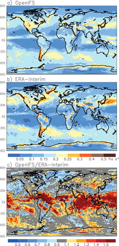
To verify that OpenIFS produces a reasonable climatology of vertical motions, the root-mean-square (RMS) amplitude of (600 hPa) is compared between the ERA-Interim reanalysis (Dee et al. 2011) and OpenIFS in Fig. 1. The RMS amplitudes are calculated over 1460 synoptic times separated by six-hourly intervals during the one-year period, thus representing the typical magnitude of instantaneous vertical motions. In both ERA-Interim and the OpenIFS simulation, the North Atlantic, North Pacific and Southern Ocean storm tracks stand out as areas with strong vertical motions, as does to a lesser extent the Intertropical Convergence Zone (ITCZ). The vertical motions over the subtropical oceans and most of the polar regions are much weaker. The largest disagreement between ERA-Interim and OpenIFS occurs in the tropics, where vertical motions are generally stronger in OpenIFS. As vertical motion is not a directly observable quantity, and is hence potentially sensitive to limitations in the reanalysis methdology, it is not known which of OpenIFS and ERA-Interim is closer to the truth. One can also note that vertical motions at the fringes of the Antarctic and Greenland ice sheets are weaker in OpenIFS than in ERA-Interim, presumably either due to weaker katabatic winds or smoother orography. The global spatial correlation between the two fields is 0.78.

Fig. 1. Root-mean-square (RMS) amplitude of (600 hPa) for the 12-month period from December 2004 to November 2005 for (a) the ERA-Interim reanalysis and (b) the OpenIFS simulation. (c) shows the ratio between OpenIFS and Era-Interim

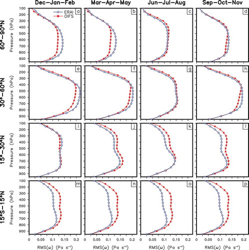
Vertical profiles of RMS amplitudes of in four latitude zones and the four standard three-month seasons are compared between ERA-Interim and OpenIFS in Fig. 2. Overall, these profiles are in good-to-excellent agreement, except for the tropics where the vertical motions are stronger in the OpenIFS simulation particularly in the mid-to-upper troposphere.

Fig. 2. RMS amplitudes of for the four standard three-month seasons and four latitude belts for the ERA-Interim reanalysis (blue) and the OpenIFS simulation (red)

Overall, we judge OpenIFS to represent well the vertical motions of the reanalysis data, although the worse agreement in the tropics than at higher latitudes also implies a somewhat lower confidence to our omega equation results in the tropics than in the other zones. By comparing our one-year period and the decade 1996–2006 in the ERA-Interim reanalysis, we have also verified that a one-year period is sufficient for deriving a reasonably good climatology of RMS() (not shown).

3. Methods

3.1. Generalized omega equation

The generalized omega equation was used in the same form as in R95:

(1)

The first four forcing terms on the right-hand side of eq. (1) represent the effects of vorticity advection (), thermal advection (), friction () and diabatic heating (). The last one () describes imbalance between vorticity and temperature tendencies. Neglecting the variation of the Coriolis parameter and moisture-related variations in the gas constant , this term is directly proportional to the pressure derivative of the ageostrophic vorticity tendency (eq. (3) in R95). Because the left-hand-side operator is linear with respect to , the contributions of the five forcing terms can be calculated separately provided that homogeneous boundary conditions ( =0 at the lower and upper boundaries, taken here as 1000 and 50 hPa) are used. The contribution of orographic vertical motions could be added by using a non-zero lower boundary condition (Krishnamurti 1968) but is not considered in this study.

3.2. Numerical solution

Eq. (1) is solved iteratively. First, the equation

(2)

is solved. Here represents any of the forcing terms in (1) and is a quasi-geostrophic version of the operator , is the area mean of the stability and s, a standard value of the Coriolis parameter. This operator can be inverted efficiently using spherical harmonics. The subsequent iterations follow

(3)

where is calculated in grid space from the previous estimate , and is the iteration step. Underrelaxation ( =0.7) was used to keep the solution stable everywhere. A total of 70 iterations were used with eq. (3). As discussed in Pauley and Nieman (1992), a unique solution of eq. (1) only exists when the operator is uniformly elliptic. To fulfill the resulting stability conditions, stability and vorticity were locally modified, as described in R95. All the pressure and spatial derivatives in the five forcing terms of (1) and in were evaluated with standard second-order finite difference approximations in the 1.5 1.5 50 hPa grid. The time derivatives in were estimated using two-hour central differences. For more details about the numerical methods, see R95.

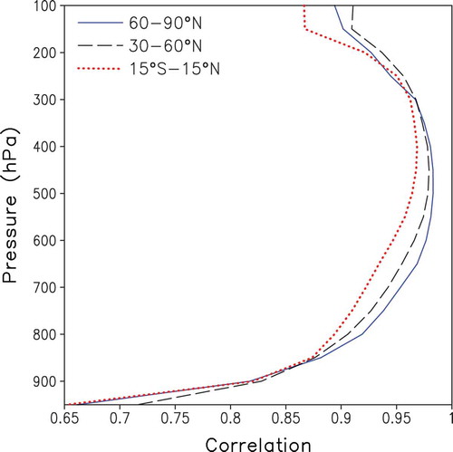
To evaluate the accuracy of the numerical solution, the spatial correlation between the calculated and OpenIFS-simulated was computed at each pressure level and for different latitude zones, for 1460 times during the one-year period. The resulting time-averaged correlations in Fig. 3 exceed 0.8 at all levels in all latitude zones and 0.95 in the midtroposphere. Values for the tropics (15S-15N) are significantly higher than in R95 (his Fig. 7(a)), most probably for two reasons. First, the higher time resolution (one hour vs. six hours) of our data set allows a better evaluation of the imbalance term ( in (1)), which turns out to be important at low latitudes. Second, R95 used a rather early analysis product from the mid-1980’s (Uppala 1986). Thus, as discussed in R95, the modest agreement found in that study might have been affected by an inconsistency between the analyzed vertical motions and the field of diabatic heating used in solving the omega equation.

Fig. 3. Average annual correlation between the generalized omega equation solution and values obtained directly from OpenIFS

4. Results

4.1. components in different latitude belts: Northern Hemisphere winter

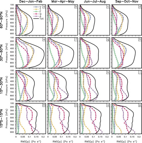
RMS amplitudes of the components and their sum () are presented in Fig. 4 for different latitude belts and seasons. In the Northern Hemisphere winter (DJF, left column of Fig. 4) at mid- (30–60N) and high latitudes (60–90N), midtropospheric vertical motions are dominated by vorticity advection () and thermal advection (). Consistent with R95, thermal advection makes a slightly larger contribution in the lower troposphere, where thermal advection is commonly strong. Conversely, the contribution of vorticity advection peaks more strongly in the upper midtroposphere, slightly below the climatological jet stream level.

Fig. 4. RMS amplitudes of (black) together with its five components for the four standard three-month seasons and four latitude belts. V corresponds to vorticity advection, T to thermal advection, F to friction, Q to diabatic heating, and A to the imbalance term.

Within the QG framework, the forcing terms associated with vorticity advection and thermal advection are often combined using vectors (Hoskins et al. 1978; Holton and Hakim 2013), with the motivation that they are not physically independent from each other. Nevertheless, our results suggest that and are nearly uncorrelated in a statistical sense. Depending on the latitude zone and season, their correlation at the 600 hPa level varies from -0.32–0.12, with values between −0.1 and −0.2 being the most common (Table 1). Similarly weak correlations are found throughout the troposphere (not shown).

Table 1. Correlation between and for different latitude belts and seasons at the 600 hPa level

15S - 15N	−0.204	−0.151	−0.168	−0.228
15N - 30N	0.119	0.0721	−0.143	−0.107
30N - 60N	−0.123	−0.149	−0.151	−0.156
60N - 90N	−0.176	−0.211	−0.316	−0.181

Diabatic heating induces much stronger vertical motions in midlatitudes than in high latitudes, as shown by RMS() in Fig. 4(a,e). This contribution is dominated by latent heat release, which is much weaker at high latitudes than midlatitudes due to the lower water vapor content. Friction () makes a substantial contribution to the vertical motions in the lowest troposphere but its contribution decreases upward above 850 hPa. Although smaller than and , the imbalance term () is comparable with the contribution of diabatic heating in the midlatitudes and it is somewhat larger than the contribution of diabatic heating in high latitudes.

Towards the equator, the contributions of thermal advection, vorticity advection and friction decrease in magnitude, whereas diabatic heating and the imbalance term grow more important. Nonetheless, thermal advection is still found to make the largest contribution to mid-to-upper tropospheric vertical motions in the subtropics (15–30N) in DJF (Fig. 4(i)). In the tropics (15S-15N), is the largest term in mid-to-upper troposphere but closer to the surface it is exceeded by (Fig. 4(m)). Notably, however, RMS() is smaller than RMS() at the lowest levels in the tropics. As discussed in the next subsection, this reflects a compensation between and .

Most of the DJF results in Fig. 4 are in good agreement with R95, particularly at mid- and high latitudes. However, the contribution of the imbalance term () is in all four latitude belts larger than indicated by R95. This is is most likely due to the fact we used 2-h time differences to estimate the time derivatives in , whereas in R95 data were only available at 6-h intervals. Furthermore, there is at least a factor of two difference in RMS() in the tropics between our study and R95, with stronger vertical motions in our case. We believe that this primarily reflects limitations in the ECMWF FGGE level IIb data set used in R95 (Uppala 1986), which apparently suffered from an underactive tropical atmosphere. This difference occurs in all five components of , but is most pronounced for and (in particular) .

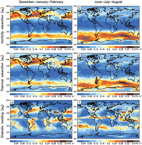
4.2. Geographical context: Northern Hemisphere winter

Winter in the Northern Hemisphere is characterized by a strong contrast in the amplitude of vertical motions between land and ocean areas (Fig. 5, left column). The highest RMS values of and are found over the North Pacific and North Atlantic storm tracks in DJF (Fig. 5(a,c)). At the other extreme, both of these terms are small in north-eastern Eurasia, where vertical motions are suppressed by stable and anticyclonic conditions. The winter maxima of over the North Atlantic and North Pacific also follow the storm track positions, but mainly in their entrance regions in the west (Fig. 5(e)). This suggests that diabatic heating is important for the vertical motions in the deepening cyclones off the east coasts of North America and Asia. Further east, where the cyclones are typically maturing and decaying, the role of diabatic heating is reduced and vertical motions are more strongly dominated by vorticity advection and thermal advection. Generally, in DJF, diabatic heating is much more important for the vertical motions over the extratropical oceans than over the continents.

Fig. 5. RMS amplitudes of , , and for DJF (a,c,e) and JJA (b,d,f) at 600 hPa

At extratropical latitudes, the imbalance forcing term () is closely proportional to the pressure derivative of the ageostrophic vorticity tendency. Therefore, this term is expected to be relatively more important in areas where high wind speeds increase the Rossby number and thus the magnitude of ageostrophic winds. The local maxima in over the North Atlantic and North Pacific storm tracks are consistent with this expectation (Figs. 6(a,c)).

Fig. 6. RMS amplitudes of for DJF (a,c) and JJA (b,d) at 600 and 900 hPa.

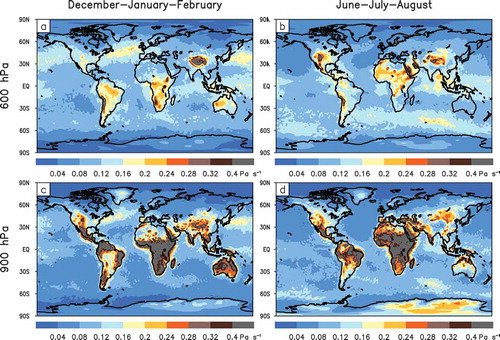
In the tropics, the imbalance term is large and it actually provides the highest RMS contribution to the vertical motions below the 750 hPa level (Fig. 4(m)). There is a strong land-sea contrast in this term at 600 hPa (Fig. 6(a)), but even more so at 900 hPa (Fig. 6(c)). As shown by eq. (1), the forcing is the sum of two parts, the first of which is associated with the vorticity tendency and the second with the temperature tendency. However, because the vorticity tendency component is proportional to the Coriolis parameter, it tends to become small close to the equator. Over the tropical continents, in particular, this leaves dominated by its temperature tendency component.

The highest values of in the tropical lower troposphere are likely to be explained by the strong diurnal cycle of temperature in the boundary layer. However, these strong vertical motions are somewhat fictitious because and tend to compensate each other. Referring to eq. (1), a local maximum of daytime diabatic heating makes positive, whereas a local maximum in positive temperature tendency makes negative in the tropics where the Coriolis parameter is small. Therefore, where and when diabatic heating is not balanced by adiabatic cooling due to rising motion but rather leads to a local warming, a compensation between and is expected.

4.3. Seasonal variability

From winter to summer, the atmosphere in the extratropical Northern Hemisphere warms considerably and its moisture content increases. Simultaneously, the meridional temperature gradient decreases and the baroclinic storm tracks become weaker and shift poleward. For vertical motions, this implies that (i) the relative importance of latent heat release should increase, (ii) the contributions of thermal advection and vorticity advection should decrease, (iii) this decrease should be less pronounced at high latitudes than further south. Furthermore, it is reasonable to expect that spring and autumn should be in most respects intermediate cases between winter and summer. All these expectations are confirmed by the results shown in the three rightmost columns in Fig. 4 and by a comparison of the winter and summer maps in Fig. 5.

In particular, the vertical motions at midlatitudes (30–60N) are markedly weaker in summer than in winter (Fig. 4(e,g)). This is mainly because both and are substantially reduced in amplitude. As RMS() is reduced much less, it exceeds RMS() and RMS() in the mid-to-lower troposphere in summer. In winter, diabatic heating is much more important for the vertical motions over the extratropical oceans than over the continents (Fig. 5(e)), but in summer this contrast largely disappears, as increasing atmospheric moisture content amplifies diabatically induced vertical motions over the continents but reduced cyclone activity suppresses them over the oceans (Fig. 5(f)). The amplitude of the imbalance term () changes little with season at the midlatitudes, but its relative importance is the largest in summer when the vertical motions as a whole are the weakest (Fig. 4(e-h)).

At high latitudes (60–90N) as well, the importance of diabatic heating increases from winter to summer, but remains secondary to and throughout the year (Fig. 4(a-d)). As expected from the poleward shift of the storm tracks in summer, the seasonal variation in the RMS amplitudes of , and is smaller in this zone than at midlatitudes. In northeastern Siberia, both and are slightly stronger in JJA than in DJF, as the vertical motions in winter are suppressed by anticyclonic conditions (Figs. 5(a-d)).

In the subtropical zone (15–30N), RMS() and RMS() are maximized in winter, particularly in the upper troposphere (Fig. 4(i-l)). This probably reflects the penetration of midlatitude baroclinic eddies into the subtropics in winter. Apart from this, the seasonal cycle is delayed from that at higher latitudes, with exhibiting its largest (smallest) amplitude in spring (in fall). The spring maximum mainly arises from a maximum in in this season. In the tropics and subtropics, the strongest diabatic heating and thus the largest values of occur over the ITCZ and the summer hemisphere monsoon regions (Fig. 5(e-f)). Furthermore, the maxima of over the low-latitude continents tend to shift northward from DJF to JJA (Fig. 6), presumably due to the stronger diurnal cycle in temperature in the summer hemisphere. However, the RMS statistics for the tropics (15S-15N) as a whole are nearly seasonally invariant (Fig. 4 (m-p)).

Our analysis has focused on the Northern Hemisphere, but the maps in Fig. 4 (a-d) also reveal a substantial increase in the amplitude of vertical motions over the Southern Ocean from DJF to JJA. Another notable detail is the pronounced maximum in the amplitude of in southern South America, particularly in the local winter (Fig. 5 (d)). This appears consistent with the fact that the lee of the Andes is a preferred region for cyclogenesis (Sinclair 1995).

4.4. Comparison between areas of rising and sinking motion

This far, the importance of the various components has been characterized with their RMS amplitudes, which are insensitive to the sign of the vertical motion. To study the roles of these components in areas of rising and sinking motion separately, their mean values were computed separately for those time steps and grid boxes in which the sum of the five components () is negative (Fig. 7(a-d)) and in which it is positive (Figs. 7(e-h)). To be concise, only the averages for the whole year are shown and discussed here.

Fig. 7. Mean values of and its five components when and where is negative (a-d) and when and where it is positive (e-h). For this figure, data for all 12 months is used. Due to the additivity of the mean values, the sum of the five components equals . Also note that the scale on the upper row is reversed.

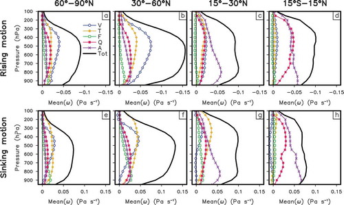
Excluding the subtropical zone (15–30N) the mean of in areas of rising motion is larger than the mean of in areas of sinking motion. Thus, where it occurs, rising motion is typically stronger than sinking motion, but it covers a smaller area. As a second general feature shown by Fig. 7, the mean values of the individual components are in a large majority of the cases of the same sign with . This is not a trivial result: if some of the five components had a strong tendency to oppose the others, it should on the average also oppose . A few exceptions occur [for example, Fig .7(h) shows that the mean of in areas of downward motion () is negative in the tropics] but none of them is large in absolute terms.

Typically, the same terms are important in both areas of upward and downward motion. Still, there are some quantitative differences. For example, in the midlatitudes, vorticity advection clearly makes a larger mean contribution than thermal advection in areas of rising motion (Fig. 7(b)). Where is downward, however, thermal advection is more important at most levels (Fig. 7(f)). These findings also apply to high latitudes (Fig. 7(a,e)). One can also note that the mean of clearly exceeds that of in areas of sinking motion in the tropics (Fig. 7(h)), and below 500 hPa the same also applies to areas of rising motion (Fig. 7(d)). These results may seem unexpected given the RMS amplitudes shown in the bottom row of Fig. 4. However, the RMS amplitudes are by construction relatively more sensitive to large local values of vertical motion (e.g., strongly negative where heavy precipitation occurs) than the mean values shown in Fig. 7.

5. Conclusions

In this paper we presented a statistical analysis of causes of atmospheric vertical motions in a one-year simulation with the OpenIFS atmospheric model. Using hourly output data from the model as input to a generalized omega equation, the vertical motions associated with vorticity advection, thermal advection, friction, diabatic heating, and an imbalance term were diagnosed. The importance of these terms was assessed by calculating their RMS amplitudes in four latitude belts as a function of pressure and season. For the most important terms, the geographical distributions of the local RMS amplitudes were also presented. Finally, the contributions of the various terms were assessed separately in areas of rising and sinking motion.

Our analysis widens and refines the study of R95, in which a similar analysis of RMS amplitudes for four latitude belts was presented based on analysis data for six synoptic times in February 1979. It confirms many of the findings in this earlier study, including the general dominance of vorticity advection and thermal advection at extratropical latitudes in winter, the increasing importance of diabatic heating towards the tropics, and the significant but not dominant role of friction in the lowest troposphere. On the other hand, our study shows that the imbalance term is more important than found in R95, basically because the higher time resolution of our data set allows a much more accurate calculation of it. This term is particularly important in the lower troposphere over tropical land areas, where the assumption of an approximate thermal wind balance between temperature and vorticity tendencies does not hold.

For the first time, we show how the statistics of vertical motion vary with season. An important although qualitatively expected finding is the increase in the relative importance of diabatic heating at the expense of vorticity advection and thermal advection at the Northern Hemisphere midlatitudes from winter to summer. The larger data set, compared to earlier studies with the generalised omega equation, also allows us to map the statistics of vertical motion components in a geographical context. This reveals, for example, broad maxima in the contributions of vorticity advection and thermal advection along the North Atlantic and North Pacific storm tracks in winter, whereas the corresponding maxima for diabatic heating are more focused in the southwestern entrance regions of the storm tracks. Finally, we find that the same terms are typically important in both areas of rising and sinking motion, although there are some quantitative differences. For example, our results suggests that, at extratropical latitudes, vorticity advection is relatively more important than thermal advection in areas or rising motion but this is reversed in areas of sinking motion. The causes of this behaviour would require further investigation.

From a methodological point of view, combining the output of a state-of-the-art atmospheric model with a diagnostic tool such as the generalized omega equation allows us to gain insight and quantitative statistics that would be difficult to obtain with reanalysis or other observation-based data alone. Naturally, as the results may be to some extent model-dependent, it would be useful to repeat a similar analysis using output from other atmospheric models. Another important topic that is within the reach of our methodology is the effect of climate change on the dynamics of atmospheric vertical motions. To study this issue, we are currently planning OpenIFS simulations with increased sea surface temperatures to mimic the first-order effects of anthropogenic climate change.

Acknowledgement

OS was supported by the Maj and Tor Nessling Foundation (grants 201400080, 201500117 and 201600119). VAS was supported by the Academy of Finland Finnish Center of Excellence program (grant 272041). We acknowledge CSC–IT Center for Science Ltd for the allocation of computational resources. We acknowledge ECMWF for making the OpenIFS code available and thank Glenn Carver, Filip Váa (ECMWF) and Juha Lento (CSC) for their assistance with running OpenIFS. The comments of two anonymous reviewers helped to improve the quality of this paper.

Disclosure statement

No potential conflict of interest was reported by the authors.

Additional information

Funding

This work was supported by the Maj and Tor Nessling Foundation; [201400080]; [201500117]; [201600119]; Academy of Finland Finnish Center of Excellence; [272041].

References

- Back, L. E., and C. S. Bretherton. 2009. A simple model of climatological rainfall and vertical motion patterns over the tropical oceans. J. Climate. 22(23), 6477–6497. DOI:10.1175/2009JCLI2393.1
- Davies, H. C. 2015. The quasigeostrophic omega equation: Reappraisal, refinements, and relevance. Mon. Wea. Rev. 143, 3–25. DOI:10.1175/MWR-D-14-00098.1.
- Dee, D., Uppala SM, Simmons AJ, Berrisford P, Poli P. and co-authors. 2011. The ERA-Interim reanalysis: Configuration and performance of the data assimilation system. Quart. J. Roy. Meteor. Soc. 137(656), 553–597. DOI:10.1002/qj.828.
- Holton, J. R., and G. J. Hakim. 2013. An Introduction to Dynamical Meteorology. 5th ed. Amsterdam: Academic Press.
- Hoskins, B. J., I. Draghici, and H. C. Davies. 1978. A new look at the ω‐equation. Quart. J. Roy. Meteor. Soc. 104(439), 31–38. DOI:10.1256/smsqj.43902.
- Jung, T., Miller MJ, Palmer TN, Towers P, Wedi N. and co-authors. 2012. High-resolution global climate simulations with the ECMWF model in project Athena: Experimental design, model climate, and seasonal forecast skill. J. Climate. 25(9), 3155–3172. DOI:10.1175/JCLI-D-11-00265.1.
- Krishnamurti, T. 1968. A diagnostic balance model for studies of weather systems of low and high latitudes, Rossby number less than 1. Mon. Wea. Rev. 96(4), 197–207. DOI:10.1175/1520-0493(1968)096<0197:ADBMFS>2.0.CO;2.
- Lorenz, E. A. 1955. Available potential energy and the maintenance of the general circulation. Tellus. 7(2), 157–167. DOI:10.1111/j.2153-3490.1955.tb01148.x.
- Pauley, P. M., and S. J. Nieman. 1992. A comparison of quasigeostrophic and nonquasigeostrophic vertical motions for a model-simulated rapidly intensifying marine extratropical cyclone. Mon. Wea. Rev. 120(7), 1108–1134. DOI:10.1175/1520-0493(1992)120<1108:ACOQAN>2.0.CO;2.
- Räisänen, J. 1995. Factors affecting synoptic-scale vertical motions: A statistical study using a generalized omega equation. Mon. Wea. Rev. 123(8), 2447–2460. DOI:10.1175/1520-0493(1995)123<2447:FASSVM>2.0.CO;2.
- Rose, B. E., and C. A. Lin. 2003. Precipitation from vertical motion: A statistical diagnostic scheme. Int. J. Climatol. 23(8), 903–919. DOI:10.1002/joc.919.
- Sinclair, M. R. 1995. A climatology of cyclogenesis for the southern hemisphere. Mon. Wea. Rev. 123(6), 1601–1619. DOI:10.1175/1520-0493(1995)123<1601:ACOCFT>2.0.CO;2.
- Uppala, S. 1986. The assimilation of the final level IIb dataset at ECWMF, Part 1. Natl. Conf. on the Scientific Results of the First GARP Global Experiment, Amer. Meteor. Soc, 24–31.