Kinetic energy generation in heat engines and heat pumps: the relationship between surface pressure, temperature and circulation cell size

ABSTRACT

The pattern and size of the Earth’s atmospheric circulation cells determine regional climates and challenge theorists. Here the authors present a theoretical framework that relates the size of meridional cells to the kinetic energy generation within them. Circulation cells are considered as heat engines (or heat pumps) driven by surface gradients of pressure and temperature. This approach allows an analytical assessment of kinetic energy generation in the meridional cells from the known values of surface pressure and temperature differences across the cell, and . Two major patterns emerge. First, the authors find that kinetic energy generation in the upper and lower atmosphere respond in contrasting ways to surface temperature: with growing , kinetic energy generation increases in the upper atmosphere but declines in the lower. A requirement that kinetic energy generation must be positive in the lower atmosphere can limit the poleward cell extension of the Hadley cells via a relationship between and . The limited extent of the Hadley cells necessitates the appearance of heat pumps (Ferrel cells) – circulation cells with negative work output. These cells consume the positive work output of the Hadley cells (heat engines) and can in theory drive the global efficiency of an axisymmetric atmospheric circulation down to zero. Second, the authors show that, within a cell, kinetic energy generation is largely determined by in the upper atmosphere, and by in the lower. By absolute magnitude, the temperature contribution is about 10 times larger. However, since the heat pumps act as sinks of kinetic energy in the upper atmosphere, the net kinetic energy generation in the upper atmosphere, as well as the net impact of surface temperature, is reduced. The authors use NCAR/NCEP and MERRA data to verify the obtained theoretical relationships. These observations confirm considerable cancellation between the temperature-related sources and sinks of kinetic energy in the upper atmosphere. Both the theoretical approach and observations highlight a major contribution from surface pressure gradients, rather than temperature, in the kinetic energy budget of meridional circulation. The findings urge increased attention to surface pressure gradients as determinants of the meridional circulation patterns.

Keywords:

• meridional circulation cells
• kinetic energy generation
• surface temperature
• surface pressure gradient
• Carnot cycle
• heat engine
• heat pump
• condensation

1. Introduction

Our planet’s meridional circulation cells determine many aspects of our climate (Bates, 2012; Shepherd, 2014). Shifting cell boundaries cause climatic changes such as the reduced rainfall observed in much of the subtropics (Webster, 2004; Bony et al., 2015). Nonetheless, what determines the extent and intensity of the Earth’s major meridional cells remains debated (Schneider, 2006; Heffernan, 2016).

On a rotating planet, such as Earth, the poleward extension of the meridional circulation cells can be estimated assuming conservation of angular momentum in the upper atmosphere. In this case, as the air moves poleward and approaches the Earth’s rotation axis, the air velocity must increase. The energy for this acceleration is derived from the temperature-induced pressure gradient: in the upper troposphere air pressure is higher over warm areas than over cold areas. The greater the meridional temperature gradient, the further it can push the equatorial air poleward.

If, rather than being conserved, the moving air’s angular momentum decreases, air velocity increases more slowly. Then, for the same temperature difference, the meridional cell can reach closer to the pole. The degree to which angular momentum is conserved is controlled by turbulent friction (eddy diffusivity), which determines the exchange of angular momentum between the atmosphere and the rest of the planet. The effects of angular momentum conservation and turbulent friction on the size of circulation cells have received attention from different perspectives (Held and Hou, 1980; Johnson, 1989; Robinson, 1997; Schneider, 2006; Chen et al., 2007; Marvel et al., 2013; Cai and Shin, 2014).

Two limiting cases have been recognized. If eddy diffusivity is zero, the meridional cells do not exist: there are westerly winds everywhere except at the surface where air velocity is zero (Held and Hou, 1980). In this case no heat engines exist and no kinetic energy is generated. If, on the other hand, turbulent friction in the upper atmosphere is sufficiently large, meridional circulation cells can extend to the poles (see, e.g. Marvel et al., 2013, their figure 3). Thus, provided turbulent friction is known, the extension and intensity of the meridional circulation cells could be found from the equations of hydrodynamics. However, turbulent friction is not simply a determinant of atmospheric circulation but is also determined by it. Since we lack an accepted general theory of atmospheric turbulence, the parameters that govern turbulent friction in circulation models cannot be specified in advance but are chosen so that circulation conforms to observations. This hampers reliable predictions of future climates.

In a steady-state atmosphere the rate at which kinetic energy of wind dissipates to heat by turbulent friction equals the rate at which this energy is generated anew by pressure gradients. But, unlike turbulence, the generation of kinetic energy can be readily formulated in terms of key atmospheric parameters.

In this paper we present an analytical approach that relates kinetic energy generation in circulation cells, viewed as heat engines or heat pumps, to surface pressure and temperature gradients and use National Center for Atmospheric Research (NCAR)/National Centers for Environmental Prediction (NCEP) (Kalnay et al., 1996) and Modern Era Retrospective Re-Analysis for Research and Applications (MERRA) (Rienecker et al., 2011) data to verify features indicated by our analyses.

In Section 2 we explore the general relationship between kinetic energy generation and work output of a heat engine operating in a hydrostatic atmosphere. The heat engine concept was applied to the atmosphere by many authors attempting to constrain the efficiency of atmospheric circulation (Wulf and Davis, 1952; Peixoto and Oort, 1992; Pauluis et al., 2000; Lorenz and Rennó, 2002; Pauluis, 2011; Huang and McElroy, 2014, 2015a, 2015b; Kieu, 2015). However, the relationship between surface pressures and temperatures and the generation of kinetic energy has not been previously established.

We derive such relationships for a Carnot cycle and for a more realistic cycle with the air streamlines parallel to the surface in, respectively, Sections 3 and 4. We show that kinetic energy generation in the lower and upper atmosphere has distinct relationships with surface temperature. For a heat engine, the greater the surface temperature difference between the warmer and the colder ends of the circulation cell, the more kinetic energy is generated in the upper atmosphere and less in the lower. (A reverse relationship holds for a heat pump.) The further the cell extends towards the pole, the greater the surface temperature difference becomes and, hence, the less kinetic energy is generated in the lower atmosphere. Thus, the requirement that kinetic energy generation in the lower atmosphere be positive limits the horizontal dimension of the cell. We express this limit in terms of surface temperature and pressure differences across the cell.

In Section 5 we evaluate the kinetic energy generation budget in the atmosphere composed of several heat engines (Hadley and Polar cells) and heat pumps (Ferrel cells). We find that the large contributions of surface temperature gradients to kinetic energy generation are of similar magnitude but of the opposite sign in heat engines and heat pumps and largely cancel each other out. The net kinetic energy generation appears determined by surface pressure gradients.

In the concluding section we discuss the importance of understanding surface pressure gradients as a necessary step towards predicting the energetics and arrangement of meridional cells. We highlight a distinct role for evaporation and condensation in the generation of surface pressure gradients as a perspective for future research.

2. Kinetic energy generation and work in a hydrostatic atmosphere

To relate kinetic energy generation to the work of a thermodynamic cycle we envisage atmospheric motion from two perspectives: the equation of motion and the thermodynamic definition of work. Taking the scalar product of the equation of motion with velocity v we obtain:

(1)

Here is kinetic energy of air per unit mass, and are air density and pressure, , and are the horizontal and vertical velocity, F is turbulent friction, and is the material derivative of X. The second equality in eq. (1) assumes hydrostatic equilibrium

(2)

In eq. (1), represents the rate of kinetic energy generation per unit air volume, while represents dissipation of this kinetic energy by turbulent processes. Equation (1) reflects the fact that in hydrostatic equilibrium kinetic energy is generated by horizontal pressure gradients (Lorenz, 1967; Boville and Bretherton, 2003; Huang and McElroy, 2015b).

We now consider a steady-state atmosphere where an air parcel of constant mass moves along a closed trajectory covering it all in time . All variables depend on altitude and one horizontal coordinate , which represents distance along the meridian. Using the definition of horizontal velocity , from eq. (1) we obtain for kinetic energy generated per mole of air (J mol), as the air moves from point at time point to at ():

(3)

Here (m mol) is molar volume, is the streamline equation and we have used the ideal gas law

(4)

where J mol K is the universal gas constant and is temperature.

On the other hand, using , and eq. (4) in the form , for total work (J mol) of the thermodynamic cycle corresponding to our closed streamline we have

(5)

as far as, first, , and, second, from eq. (2) we have

(6)

Here is molar mass of air, and and are the equations of the closed streamline that defines the cycle.

Equation (5) shows that for any thermodynamic cycle where the mass of gas is constant, total work A is equal to total kinetic energy generation K (obtained when integration in eq. (3) is made over the entire streamline) – and this depends solely on horizontal pressure gradients. In an atmosphere where water vapor undergoes phase transitions, eq. (5) still describes kinetic energy generation (but not total work) with reasonable accuracy (see Appendix A for details). [For an arbitrary part of the streamline kinetic energy generation is not equal to work performed by the air as it moves from with temperature to with temperature , because in this case neither the temperature integral, , nor the integral in eq. (6), , are zero.]

Equation (3) applies to rotating as well as to non-rotating planets. As Coriolis force is perpendicular to air velocity, it does not make any contribution to eq. (1) or wind power (kinetic energy generation per unit time). Thus, while wind velocity may be found assuming geostrophic balance, wind power cannot. Wind power is non-zero only if the geostrophic balance is broken.

3. Kinetic energy generation and cell size limit in a Carnot cycle

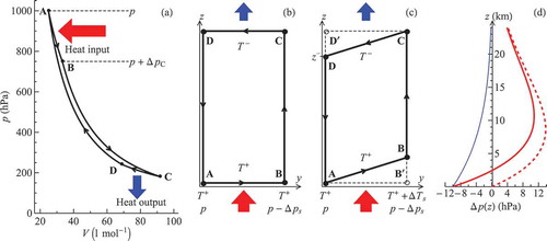
A Carnot cycle consists of two isotherms and two adiabats (Fig. 1a). Work outputs on the two adiabats have different signs and sum to zero. Total work output is equal to the sum of work outputs on the two isotherms and can be written as

(7)

Fig. 1. Hydrostatic Carnot heat engine. (a) Carnot cycle with typical atmospheric parameters: hPa, K (isotherm AB), K (isotherm CD), hPa. Work output at the warmer (colder) isotherm is equal to heat input (output). BC and DA are adiabats. (b, c) The same cycle in spatial coordinates , in (b) horizontally isothermal atmosphere ( K) and (c) in the presence of a horizontal temperature difference ( K). (d) Differences in pressure at height for atmospheric columns above points and , where pressure and temperature follow eqs. (9) and (8) with surface pressure and temperature at points and equal to hPa, K and , ; thin solid blue curve: hPa, K; dashed red curve: hPa, K; thick solid red curve: hPa, K.

Here and are the temperatures of the two isotherms, p is the pressure that the air has as it starts moving along the warmer isotherm and is the pressure change along the warmer isotherm, (for a derivation, see, e.g. Makarieva et al., 2010). If the air expands at the warmer isotherm (cycle ABCDA), we have and . The Carnot cycle is then a true heat engine: it does work on the external environment and transports heat from the heat source to the heat sink (Fig. 1a). If the air contracts at the warmer isotherm (cycle BADCB) we have and . The Carnot cycle functions now as a heat pump: it transports heat from the heat sink (cold area) to the heat source (warm area) consuming work from the external environment.

We consider a closed streamline where the adiabats are vertical. If the atmosphere is horizontally isothermal, then the isothermal parts of the streamline lie parallel to the surface and the work output of the cycle is determined by surface pressure difference (Fig. 1b). If there is a horizontal temperature gradient at the surface, then the isotherms are no longer horizontal, but have an inclination that depends on the magnitude of the vertical temperature lapse rate (Fig. 1c). In this case depends on differences in surface pressure and temperature as well as on the lapse rate.

We consider a hydrostatic atmosphere with a constant lapse rate , where temperature and pressure depend on y and z:

(8)

(9)

Subscript s denotes values of pressure and temperature at the Earth’s surface. Equation (9) derives from eq. (8) and the condition of hydrostatic equilibrium (2) (for a derivation see Makarieva et al., 2015c). It describes a dry adiabat K km^–1 as a special case, but is equally valid for any constant . In particular, putting K km^–1 (the mean tropospheric lapse rate) we can approximately account for the latent heat release that occurs in the Earth’s moist atmosphere. In Appendix B we discuss how our assumption of being invariant with regard to z and y affects our results.

Consider a cycle with positive total work as in Fig. 1c. Given the small relative changes of surface pressure and temperature we can write their dependence on y in the linear form:

(10)

where , , , , , and .

Streamline equations for the warmer isotherm AB with temperature and the colder isotherm CD with temperature are obtained from eqs. (10) and (8):

(11)

(12)

Differentiating eq. (9) over y for constant z and using eqs. (10)–(12) we obtain from eq. (3) the following expressions for kinetic energy generation and at the warmer and colder isotherms, respectively:

(13)

(14)

As we discuss below, typical relative differences and are small ( and ). Therefore, all calculations in eqs. (13) and (14) can be done to the accuracy of the linear terms over and linear and quadratic terms over . Integrating eqs. (13) and (14) and expressing the result in these approximations we obtain:

(15)

(16)

(17)

Here and are the total work outputs on isotherms AB and CD, respectively; and are surface pressure and temperature at point , and and are pressure and temperature at point . Equation (17) can also be obtained from eq. (7) with the use of eqs. (8) and (9) and noting that and .

Equations (15)–(17) show that kinetic energy generation , and total work , on the two isotherms may have different signs. In particular, at the warmer isotherm kinetic energy generation can be either positive (at small ) or negative (at large ), while total work is always positive at large , which reflects the fact that gas expands at the lower isotherm.

For a horizontally isothermal surface with (Fig. 1b) we have and , i.e. kinetic energy generation at the colder isotherm is negative. This means that in the upper atmosphere the air must move towards higher pressure (see Fig. 1d, solid blue line), thus losing kinetic energy. At the beginning of this path (at point ) the air must possess kinetic energy exceeding to cover the entire isotherm CD. If the kinetic energy is insufficient, at a certain point between and it will reach zero. The air will start moving in the opposite direction under the force of the pressure gradient. For K and hPa we have J mol or J kg, where g mol is molar mass of air. This corresponds to an air velocity of about m s. Such velocities are common in the upper troposphere, which means that the cycle shown in Fig. 1b is energetically plausible.

Now consider a situation when , but . The relationship between work outputs is reversed: kinetic energy generation is negative at the warmer isotherm, , and positive at the colder isotherm, . This is because at all heights, except at the surface, air pressure is higher in the warmer area towards which the low-level air is moving (Fig. 1d, red dashed line). Thus, now the air must spend its kinetic energy at the warmer isotherm to overcome the opposing action of the horizontal pressure gradient force. Using a typical value of K in the Hadley cells for K, K km [, see eq. (8)] from eq. (15) we obtain J kg. This means that to travel from to the velocity of the air must exceed m s. This significantly exceeds the characteristic velocities observed in the boundary layer, which are about 8 m s (e.g. Lindzen and Nigam, 1987; Schneider, 2006, his figure 1a, b). Since in the lower atmosphere the air must also overcome surface friction, total kinetic energy required to move from to with is larger than estimated from eq. (15).

If the air’s kinetic energy is negligible compared with what is needed to move from A to B, the required kinetic energy must be generated on the warmer isotherm. For kinetic energy generation on the warmer isotherm to be positive (), surface pressure and temperature differences and must satisfy

(18)

For K and K, which characterize the surface temperature differences between the equator and the poles, at hPa and K km () we find that to satisfy eq. (18) the surface pressure difference between the equator and the pole must exceed 100 hPa. Such a pressure difference on Earth can be found in intense compact vortices such as the severest hurricanes and tornadoes; it is an order of magnitude larger than the typical in the two Hadley cells (Fig. 2b), which together cover over half of the Earth’s surface.

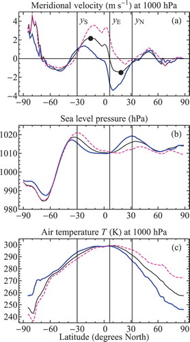
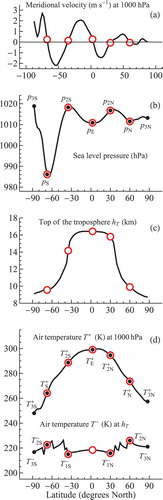
Fig. 2. Long-term mean zonally averaged meridional velocity, sea level pressure and air temperature at 1000 hPa calculated from MERRA data. Black, thick blue and pink dashed curves denote annual mean, January and July data, respectively. Black circles in (a) indicate velocity maxima; , and are the Hadley cell outer and inner borders (for details see Appendix D).

Using eq. (18) we can express the maximum size of the cell in terms of surface pressure and temperature gradients , :

(19)

For the Carnot cycle, the maximum cell size grows with an increasing surface pressure gradient and diminishes proportionally to the squared surface temperature gradient. The surface temperature gradient is approximately known: it reflects the differential solar heating that makes the pole colder than the equator. Therefore, the key to predicting cell size is to understand surface pressure gradients.

4. Thermodynamic cycle with rectangular streamlines

In a Carnot cycle, the term in the expression for kinetic energy generation is quadratic; see eqs. (15), (18) and (19). This results from the dual nature of the relationship. First, determines the mean height of the warmer isotherm via the streamline eq. (11): the greater , the greater the mean height at which the air moves in the lower atmosphere. Second, determines a pressure difference that acts as a sink for kinetic energy in the lower atmosphere (see Fig. 1d, dashed line). This pressure difference increases linearly with small and with height. This double effect leads to the negative quadratic term in eq. (15), which diminishes the rate at which kinetic energy is generated in a heat engine.

We shall now consider kinetic energy generation in such a thermodynamic cycle where the vertical adiabats are connected by horizontal streamlines. The air moves parallel to the surface at a certain height that is independent of . It is a cycle with streamlines as shown in Fig. 1b but in the presence of a surface temperature difference as in Fig. 1c.

Using eqs. (3), (8) and (9) we find that in this case kinetic energy generation along the horizontal streamlines is given by

(20)

which, using eq. (10), becomes

(21)

For the lower AB and upper CD streamlines, kinetic energy generation is calculated from eq. (21) as follows: and , respectively, where and are the altitudes of these streamlines, and .

Retaining linear terms over and [thus discarding the last term in eq. (21)] for and we find

(22)

(23)

(24)

We recognize that in the second equality in eq. (22). Note that [see eq. (8)].

Equation (22) coincides with eq. (15) for a Carnot cycle () if is equal to the mean height of the lower isothermal streamline (Fig. 1c). For the upper streamline eq. (23) coincides with , eq. (16), if we put , where and , Fig. 1. Under this assumption total work of this cycle coincides with total work of a Carnot cyle, eq. (17). [It can be shown using eqs. (9) and (8) that the efficiency of the ‘rectangular’ cycle is lower by a small magnitude of the order of .] As in a Carnot cycle, the contribution of temperature difference to kinetic energy generation is negative at the lower streamline, cf. eqs. (22) and (15), and positive at the upper streamline, cf. eqs. (23) and (16). But this negative contribution is not quadratic but linear.

From eq. (22) the condition that takes the form

(25)

(26)

Here is the atmospheric scale height and is the isobaric height at which the pressure difference between two atmospheric columns turns to zero (Makarieva et al., 2015c). Equation (26) indicates that the height where the low-level air moves must be smaller than the isobaric height. Since increases as the cell extends towards the pole, for to be constant, must grow with . If grows more slowly than , then at a certain height can turn to zero or, at constant , becomes negative. The dependence between and thus dictates the maximum cell size as long as is positive. In Appendices B and C we discuss how eq. (25) and its implications are affected by our assumptions of rectangular air trajectories and constant lapse rate.

Our analysis of monthly averaged and across Hadley cells based on MERRA data for 1979–2014 does indeed suggest a link between the ratio and cell size (see Appendix D). In those months when the meridional extension of the cells is smaller than the long-term mean, and are roughly proportional to each other. As the meridional extension of the cells increases, appears to reach a plateau becoming independent of . These emerging patterns require a more detailed analysis at various spatial and temporal scales.

5. Kinetic energy generation in the meridional circulation

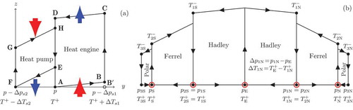
If the poleward extension of a cell with positive total work output (a heat engine like the Hadley cell) is limited, another cell with a negative work output (a heat pump) must occur poleward of it. This follows from continuity: in the adjacent cells the air must descend along DA (see Fig. 3a). Hence, in the lower atmosphere the air must move from the warmer to the colder region. Such a heat pump requires an external supply of work, which is provided by neighboring heat engines. The Earth’s Ferrel cells are heat pumps, while the Hadley and Polar cells are heat engines (see, e.g. Huang and McElroy, 2014).

Fig. 3. Heat pumps and heat engines. (a) A Carnot heat pump (cycle EFGHE) bordering with a Carnot heat engine (cycle ABCDA). See Fig. 1 for details. (b) The meridional circulation cells on Earth as approximated by eqs. (27) and (28). Arrows show the direction of air movement. Empty red circles indicate the latitude of cell borders as determined from meridional velocity values (see Fig. A5a in Appendix D). Black circles show where temperature and pressure values used in eqs. (27) and (28) were calculated: for we have , ; , ; , (see Fig. A5b and c in Appendix D). The vertical dimension is height , the horizontal dimension is sine latitude, which accounts for cell area.

We can apply the relationships developed in the previous sections to estimate kinetic energy generation in the meridional circulation as a whole. We view each cell as a thermodynamic cycle where in the lower atmosphere the air moves parallel to the surface at a height km, while in the upper atmosphere it moves parallel to the top of the troposphere (see Appendix B for a discussion of the validity of this assumption). Air temperature at the top of the troposphere, , is relatively constant across the cells, while the height of the troposphere (which is a proxy for cell height ) is halved within the Ferrel cells (see Fig. A5 in Appendix D). This justifies the use of the Carnot formula, i.e. eq. (16) rather than eq. (23), for the streamlines in the upper atmosphere. We thus approximate each of the six meridional cells as a ‘hybrid’ thermodynamic cycle with a horizontal streamline and kinetic energy generation [eq. (22)] in the lower atmosphere and an isothermal streamline and kinetic energy generation [eq. (16)] in the upper atmosphere (Fig. 3b).

Since we shall use two different equations, eqs. (22) and (16), to describe total kinetic energy generation within each of the six cycles, it is convenient to represent global kinetic energy generation as a sum of two terms. For the lower atmosphere using eq. (22) we have:

(27)

Here summation is over the six cells, three in the Southern () and three in the Northern () Hemisphere, for Hadley, Ferrel and Polar cells, respectively; and stand for the differences in surface temperature and pressure within the cell; and are surface temperature and pressure at the beginning of the lower streamline (Fig. 3b). We account for cell area (and thus approximately for the mass of circulating air) by introducing coefficients , which is the relative area of the cell with respect to the area of the hemisphere. Here and are the latitudes of cell borders closest to the equator (E) and pole (P). For Polar cells °, so .

The coefficient differentiates heat engines () from heat pumps () (Table 1). For a ‘rectangular’ heat pump where low surface pressure is associated with low surface temperature, such that the air compresses at the lower streamline, the temperature terms in eqs. (22) and (23) change their sign. (The pressure terms do not change their sign if, as in the heat engine, the low-level air moves from high to low surface pressure.) In a heat pump the temperature difference makes a negative contribution to kinetic energy generation in the upper atmosphere and a positive contribution in the lower atmosphere (Table 1). Thus, kinetic energy generation in the lower atmosphere should be greatest in heat pumps.

Table 1. Contributions of surface pressure and temperature differences to kinetic energy generation for hybrid cycles that have isothermal streamlines in the upper atmosphere [eq. (16)] and horizontal streamlines in the lower atmosphere [eq. (22)]

	Pressure	Temperature
	All cells	Heat engines	Heat pumps
Upper atmosphere
Lower atmosphere
Total atmosphere

For heat pumps the expression is valid for , cf. eq. (29).

For the upper atmosphere using eq. (16) we have

(28)

(29)

Here for is kinetic energy generation in the heat engines (Hadley and Polar cells), eq. (16); is kinetic energy generation in the heat pumps (Ferrel cells). It can be obtained following the procedure that yielded eq. (16) but for the isotherm GH instead of CD (Fig. 3a).

We used monthly NCAR/NCEP re-analysis data to calculate total kinetic energy generation (see Appendix D). In the lower atmosphere we find that J mol is determined by surface pressure differences, which make positive contributions to in all cells (Table 2). The contribution of the temperature term is virtually zero, for km (boundary layer) in eq. (27) it constitutes J mol. The absolute magnitude of the contributions of within individual cells is substantially smaller than that from : it is positive in Ferrel cells and negative in Hadley cells, contributing about 20% of by absolute magnitude.

Table 2. Budget of global kinetic energy generation (J mol) calculated from eqs. (27) and (28) using km, ( K km) and the annual mean values of all the other parameters in eqs. (27) and (28) (Fig. A5)

	Lower atmosphere			Upper atmosphere				Lower and upper atmosphere
	Total			Total						Total
Ferrel	44 ± 5	30 ± 4	14 ± 2	–152 ± 23	–23 ± 3	–111 ± 17	–18 ± 4	–97 ± 16	7 ± 2	–108 ± 18
Hadley	9 ± 1	20 ± 2	–11 ± 1	108 ± 11	–15 ± 1	116 ± 11	7 ± 1	105 ± 10	5 ± 1	117 ± 11
Polar	2 ± 2	6 ± 3	–4 ± 2	19 ± 4	–5 ± 3	18 ± 4	6 ± 4	14 ± 4	0.7 ± 0.3	21 ± 4
Ferrel + Hadley	53 ± 6	50 ± 6	3 ± 2	–44 ± 21	–38 ± 4	5 ± 18	–11 ± 4	8 ± 17	12 ± 2	9 ± 18
All cells	55 ± 6	56 ± 5	–1 ± 3	–25 ± 23	–43 ± 3	23 ± 18	–5 ± 7	22 ± 16	13 ± 2	30 ± 19

Uncertainty represents the standard deviation for monthly variation (see insets in Fig. A1). ‘Total’ in the last column includes the contribution from the upper atmosphere (this term is absent in the lower atmosphere).

Total kinetic energy generation in the upper atmosphere is negative, J mol. Surface pressure differences make negative contributions in all cells, while the surface temperature contributions are positive in the Hadley and Polar cells and negative in the Ferrel cells. The linear temperature term is also the most variable: this variability is both spatial and temporal, reflecting seasonal migration of cell borders.

Global kinetic energy generation is J mol. This is 25% of what is generated by the Hadley system ( J mol). This is consistent with the analysis of Kim and Kim (2013), who found that the net global meridional kinetic power in NCAR/NCEP re-analysis is slightly positive, albeit different methods of calculations gave different results: and W m. Assuming that the Hadley system contributes W (Huang and McElroy, 2014) or W m globally, we conclude that in the NCAR/NCEP re-analysis the net meridional kinetic power is 15–25% of the kinetic power in the Hadley system. This is in agreement with our results that are based on NCAR/NCEP data: obtained from eqs. (27) and (28) (Table 2).

An equality between the ratios of power (W) and work output (J mol) in two thermodynamic cycles () implies an equality between the amounts of gas circulating per unit time along the considered streamline in each system: , where (mol) is the number of moles circulating along the considered streamline in the th circulation, and is the time period of the cycle. Thus, if then . We have weighted kinetic energy generation in each cell by relative cell area , which reflects atmospheric mass within the cell; see eq. (27). Since , we have , where and are the number of air moles within the cell and the atmosphere as a whole, respectively. Therefore, if the ratio of power to kinetic energy generation coincides between any two circulation patterns, this means that the characteristic times of air circulation along the considered streamlines within the cells should coincide as well.

In particular, for the Hadley cells and Ferrel cells kinetic energy generation is approximately equal (but of different sign) (Table 2). The same is true for the circulation power (Huang and McElroy, 2014). This means that characteristic times of air circulation (i.e. the time during which the air completes the closed trajectory) within these systems should be similar as well. This conclusion is in agreement with the observation that meridional extent and meridional velocities in the Hadley and Ferrel cells are similar (about 30° and 2 m s in the Southern cells) (see Fig. A5a in Appendix D). Thus, at least for the horizontal part of the streamlines the time air takes to cover it is similar among the cells.

The estimated value of is sensitive to the uncertainty in the determination of the position of cell borders. Since Ferrel cells have a negative work output, and Hadley and Polar cells positive, increasing the size of the heat engines by pushing the Hadley cell border towards the poles or Polar cell border towards the equator would increase our estimate of global kinetic energy generation. Conversely, increasing area of Ferrel cells would decrease . Since cell borders are located where the meridional pressure gradient is about zero (Fig. A5b), the pressure contribution to is relatively robust and little affected by the uncertainty in determining the cell borders. However, the surface temperature gradient is steep between the Polar and Ferrel cells, so any uncertainty in the determination of these cell borders will affect the magnitude of the temperature contribution to . In consequence, the estimates of kinetic energy generation in the Polar cells are least accurate: these cells are very small (), so any border extension towards the equator not only increases temperature difference across them, but also significantly affects the relative cell area .

The estimate of derived from the NCAR/NCEP data includes a significant contribution from the Polar cells (because the larger contributions from the Hadley and Ferrel cells cancel out). The area of the Polar cells is about one-tenth of the area of Hadley cells, , while the temperature difference is about two times greater, . Thus, kinetic energy generation in the Polar cells appears to be about one-fifth of what is generated in Hadley cells (Table 2). This is of the order of the difference between kinetic energy generation in Hadley and Ferrel cells. If Polar cells are excluded from consideration, total kinetic energy generation in the remaining four cells diminishes threefold to less than 8% of what is generated by Hadley cells (cf. the last two lines in Table 2). Because of this uncertainty the sign of the total kinetic energy generation cannot be robustly established in our analysis. This uncertainty is not, however, restricted to our approach; it also reflects the insufficient quality of the available observations. Indeed, unlike in the NCAR/NCEP data, in the MERRA re-analysis the total meridional kinetic power is negative: or W m (Kim and Kim, 2013), which means that in this re-analysis the Ferrel cells consume more kinetic power than the Hadley cells produce (Huang and McElroy, 2014). The pattern common to both MERRA and NCAR/NCEP data sets is that most kinetic energy generated by the meridional heat engines is consumed by the meridional heat pumps. This robust pattern is reproduced by our analysis (Table 2).

6. Discussion and conclusions

We have derived expressions for how kinetic energy generation in the boundary layer and in the upper atmosphere depends on surface pressure and temperature differences and along the air streamline [eqs. (15) and (16)]. Our expressions are valid for any air parcel following a given trajectory irrespective of planetary rotation. We applied the derived relationships to analyze kinetic energy generation in Earth’s meridional circulation cells. We found that a typical meridional surface temperature difference makes a larger contribution to total kinetic energy generation in a circulation cell than a typical surface pressure difference (Table 1). In particular, for the Hadley cells the pressure contribution is less than 5% of the temperature contribution (Table 2, last column).

However, as we have shown, the surface temperature gradient plays a double role. The pressure gradient it generates in the upper atmosphere can be either a source or a sink of kinetic energy – this depends on whether the upper-level air moves towards the pole (lower surface temperatures) or towards the equator (higher surface temperatures). In the first case we have a heat engine with a positive work output, in the second a heat pump with a negative work output (Fig. 3a).

These relationships explain why the efficiency of the Earth’s atmosphere as a heat engine cannot reach Carnot efficiency. An ideal atmospheric Carnot cycle on Earth consuming surface heat flux W m at surface temperature K and releasing heat at with K would generate kinetic energy at a rate of W m. Recognition that the actual rate of kinetic energy generation on Earth is several times smaller urged a search for the underlying processes (e.g. Pauluis, 2011; Schubert and Mitchell, 2013). Here we have shown that in the presence of a surface temperature gradient along which several circulation cells are operating, the global efficiency of kinetic energy generation can never reach Carnot efficiency. The heat pumps with their negative work output can in theory reduce the global atmospheric efficiency to zero. For an atmosphere containing many meridional circulation cells a Carnot efficiency can be achieved if only the planetary surface is isothermal and all cells are represented by Carnot cycles with and K (Fig. 1b).

Our analyses indicate that Ferrel cells consume most of the kinetic energy generated by the Hadley cells (Table 2). This is consistent with observations (Kim and Kim, 2013; Huang and McElroy, 2014). This compensation largely reflects the cancellation of large energy sources and sinks in the upper atmosphere. For such a cancellation to occur, the positive temperature contribution in the heat engines must compensate the negative temperature contribution in the heat pumps as well as the negative pressure contribution in both heat pumps and heat engines (Table 1). As a perspective for further research we suggest that this compensation may result from a dynamic constraint which determines that the export/import of kinetic energy from/to the upper atmosphere is small. For a given distribution of surface pressure and temperature, this condition constrains height and temperature of the upper streamlines (Table 1). In other words, the observed height of the troposphere as well as the isobaric height can be constrained by the condition that total kinetic energy generation in the upper atmosphere is small compared with its value within the Hadley cells: , see eqs. (27)–(29). We have previously suggested that rather than these heights being the cause of the ratio between surface pressure and temperature differences as commonly assumed (e.g. Lindzen and Nigam, 1987; Sobel and Neelin, 2006; Bayr and Dommenget, 2013), they are its consequence (Makarieva et al., 2015c).

The temperature contribution to global kinetic generation in the lower atmosphere is also relatively small: first, because of the small factor [eq. (25)]; and second, because it is of different sign in heat pumps and heat engines (Table 1). Thus, when kinetic energy generation in the upper atmosphere is negligible, global kinetic energy generation is determined by surface pressure gradients. Our analysis highlights that the surface pressure gradients are not set by surface temperature gradients, as sometimes assumed (e.g. Lindzen and Nigam, 1987; Sobel and Neelin, 2006), but are independent parameters.

As the pole is colder than the equator, the temperature difference across the meridional circulation cell grows with increasing meridional cell extension . The obtained theoretical expression for shows that if the surface pressure difference remains constant, will decrease linearly with growing . In such a case the condition that in the boundary layer must be positive will limit the cell size.

Indeed, increasing L at constant leads to a decrease in kinetic energy generation at any given height in the boundary layer. But cannot be less that a certain positive value corresponding to friction losses. Thus, as soon as this lower limit is reached, a larger cell becomes impossible. Conversely, if surface friction is reduced, the poleward cell extension can grow, an effect noted in a modelling study by Robinson (1997). Our analysis explains this effect. Meanwhile, in the upper atmosphere turbulent friction has an opposite effect on cell size: as friction increases, the poleward cell extension grows (Marvel et al., 2013).

Our analysis of monthly MERRA data suggests that in Hadley cells does indeed grow with , but that reaches a plateau at some intermediate values of beyond which it does not grow further. Further studies are needed to verify this pattern at different spatial and temporal scales. If does indeed limit meridional cell size, the question arises what determines . In a moist atmosphere surface pressure is influenced by evaporation, condensation and precipitation. We have previously suggested that the pressure differences observed in condensation-driven circulation cells should be of the order of the partial pressure of water vapor at the surface (Makarieva et al., 2013, 2014). Since partial pressure of atmospheric water vapor grows with global surface temperature, pressure differences across the Hadley cells could increase, leading them to extend further towards the poles in a warmer climate. We thus call for a broader assessment of the impact of evaporation, condensation and precipitation on surface pressure gradients and the energetics of meridional circulation.

Acknowledgment

The authors thank two anonymous referees for constructive comments. This work is partially supported by the University of California Agricultural Experiment Station, Russian Scientific Foundation Grant 14-22-00281, the Australian Research Council project DP160102107 and the CNPq/CT-Hidro - GeoClima project Grant 404158/2013-7.

Disclosure statement

No potential conflict of interest was reported by the authors.

Additional information

Funding

This work was supported by the University of California Agricultural Experiment Station, Russian Scientific Foundation; Australian Research Council; CNPq/CT-Hidro - GeoClima.

Appendix A.

Work in the presence of phase transitions

Here we show that eq. (5) accurately describes kinetic energy generation in the presence of phase transitions. Consider an air parcel occupying volume and containing a total of moles of dry air and water vapor (subscript and , respectively). This air parcel moves along a closed steady-state trajectory which can be described in coordinates (e.g. Fig. 1a). As far as , the total work performed by such an air parcel per mole of dry air is

(A1)

Here is the change in the amount of air due to phase transitions of water vapor. Unlike in eq. (5), (subscript refers to the presence of phase transitions) is not a unique function of the integral (determined by the area enclosed by the closed streamline in the diagram): also depends on where the phase transitions occur. The diagram lacks this information.

Using the ideal gas law (4), the hydrostatic equilibrium (2) and considering that , we find

(A2)

(A3)

Here . The second integral in eq. (A3) reflects the difference between the air mass (kg) that is rising () and descending () along the trajectory. This difference is unrelated to kinetic energy generation: it is caused by phase transitions (condensation and evaporation) that in the general case occur at different heights (for further details, see Makarieva et al., 2015a, 2015b).

We conclude that in the presence of phase transitions, total work output is not equal to kinetic energy generation because of the non-zero second integral in eq. (A3), . However, kinetic energy generation as described by the first integral in eq. (A3) coincides with [eq.(5)] with good accuracy because of the small value of .

Appendix B.

Validity of the theoretical approach

Our derivations have assumed an atmosphere with a constant lapse rate and isothermal or horizontal air trajectories in the upper and lower atmosphere. We now examine how these assumptions affect our two main findings: first, the dependence of cell size on surface pressure and temperature gradients, eqs. (18) and (26); and second, that the balance between kinetic energy generated by heat engines and consumed by heat pumps reflects surface temperature gradients (Tables 1 and 2).

The first finding is based on the expression for kinetic energy generation in the lower atmosphere. Since as described by eq. (22) is linear over , and (height of air motion), eq. (22) with can be applied to any trajectory of air motion with a sufficiently small mean height . This is because even if the lapse rate varies horizontally and/or vertically, the smallness of will ensure that (air temperature is approximately equal to surface temperature) in the pressure term in eq. (22). For km and a typical tropical ratio (Lindzen and Nigam, 1987; Bayr and Dommenget, 2013; Makarieva et al., 2015c), the pressure term dominates the value of [eq. (22)]. In Appendix C we show that spatial variation in lapse rate has a comparatively minor influence.

Figure A1 shows that most kinetic energy in the lower half of the troposphere is generated within a narrow boundary layer: the rate of kinetic energy generation diminishes linearly with increasing altitude approaching zero for km (the Northern Ferrel cell is an exception discussed below). If within this layer the distribution of air pressure conforms to our eq. (9) (which assumes a constant lapse rate), then our formula for kinetic energy generation in the lower atmosphere , eq. (22), is reasonable (in calculations in Table 2 we used km). Indeed, Fig. A1a and b shows that in the Hadley cells in the lowest 2 km the observed pressure difference across the cell is very close to the theoretical pressure difference calculated from eq. (9). The reason is that the pressure scale height [eq. (26)] is governed by surface temperature, such that whatever differences in lapse rates, given is small, they cannot significantly change this height in the boundary layer.

In the Northern Ferrel cell the generation of kinetic energy is not confined to 2 km above the sea level (presumably because this cell includes considerable areas of raised land) (Fig. A1c). In this cell our theoretical relationship overestimates pressure difference in the lower troposphere: at km the theoretical estimate is about times larger than the observed pressure difference (Fig. A1c). However, since the mean height where kinetic energy is generated in the lower part of the Northern Ferrel cell is approximately twice the value of km that we assumed for all cells, the two inaccuracies partially cancel each other in the resulting estimate for kinetic energy generation in the lower atmosphere (Table 2).

In the upper atmosphere the discrepancy between the theoretical and observed pressure distributions appears more significant: over this larger range in altitude the lapse rate variation clearly matters. For the Hadley cells, the theoretical and observed pressure difference are similar from up to , where is the height where kinetic energy generation is maximum (Fig. A1a and b). For the observed pressure difference declines more rapidly. However, the theoretical pressure difference at the top of the troposphere , which we used as a proxy for the upper streamline, practically coincides with the observed pressure difference at (Fig. A1). In the Ferrel cells the discrepancy between the theoretical and observed pressure distribution is larger than in the Hadley cells but does not exceed 30%.

Further evidence that eq. (28) successfully captures the dependence of kinetic energy generation in the upper atmosphere on surface temperature differences is provided by the seasonal variation in , as shown in the insets in Fig. A1. For the heat engines, maximum kinetic energy generation is attained in the Northern (Southern) Hadley cell in January (July), when the meridional temperature gradient and, hence, the temperature difference across the cell are at their maximum (see Fig. 2c). For the heat pumps, in the Northern (Southern) Ferrel cell kinetic energy generation is also maximum by absolute magnitude in January (July), but here it is negative. These patterns conform to our theoretical relationships summarized in Table 1. There is also considerable agreement in the seasonal variability of our theoretical kinetic energy generation and the observed kinetic power output in Hadley and Ferrel cells (Fig. A1).

Overall, Fig. A1 indicates that eqs. (27) and (28) provide a reasonable first-order estimate for the relationship between kinetic energy generation in the Earth’s meridional circulation systems.

Appendix C.

Spatial variation of lapse rate in the lower atmosphere

Here we show that eq. (25) remains valid in the presence of spatial variation in temperature lapse rate, if under we understand the horizontal temperature difference at one-half the mean height of the lower streamline. In the formulae below , , where is surface temperature, is surface pressure and .

Using these relationships we find

(C1)

(C2)

Expanding the logarithm in eq. (C2) over

(C3)

we find from eq. (C3) (note that and )

(C4)

When is integrated over the boundary layer of a fixed height, i.e. when , the last term in eq. (C4) vanishes.

Noting that , and and that we defined , the kinetic energy generation in the presence of lapse rate variation becomes, cf. eq. (25):

(C5)

(C6)

Here is the horizontal temperature difference at a height equal to one-half of the mean streamline height .

Equation (C5) indicates that with a small km any horizontal variation in lapse rate makes a minor contribution to kinetic energy generation. (The vertical variation in is zero in the first approximation, again because is small). For example, even if in the boundary layer the lapse rate changes by K km (which is approximately the difference between the dry and moist adiabatic lapse rates), the lapse rate term in eq. (C5) is negligible compared with the pressure term: .

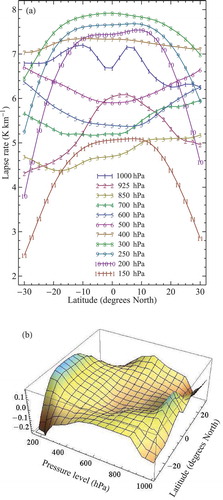
In the real atmosphere the horizontal variation in lapse rate is smaller. For example, the zonally averaged lapse rate between 925 and 850 hPa changes across the Hadley cells by about K km (Fig. A2). The lower atmosphere of the equatorial areas of the Hadley cells has a larger lapse rate than at the higher latitudes (). As follows from eqs. (C5) and (C6), a positive lapse rate difference diminishes the horizontal temperature difference and thus slightly increases the kinetic energy generation within the Hadley cells.

In hurricanes the horizontal variation in lapse rate in the boundary layer can reach K km (e.g. Montgomery et al., 2006, their figure 4c): as the air spirals in towards the hurricane center, the lapse rate diminishes, . This makes a negative contribution to kinetic energy generation. But in these systems , which is several times greater than in the zonally averaged cells, so the pressure term in eq. (C5) remains dominant. These considerations add further support to the view that kinetic energy generation in the lower atmosphere is determined by surface pressure gradients.

Appendix D.

Data and methods

For our analysis of the dependence between differences and of surface temperature and pressure in Hadley cells we used the MERRA monthly data set MAIMCPASM 5.2.0 downloaded for the years 1979–2014 (one file for each month) from http://mirador.gsfc.nasa.gov. This data set has a resolution of ( grid cells). We thus obtained data for 432 months. For each month, sea level pressure, air temperature at 1000 hPa and meridional velocity at 1000 hPa were zonally averaged excluding grid cells corresponding to land area.

Cell borders were defined as follows: for each month we first established the long-term mean position of the maxima of zonally averaged sea level pressure at the outer borders of the cells; then for each month in each year we defined the inner border of the cells as the latitude of minimum zonally averaged sea level pressure located between the long-term maxima (Fig. 2). Sea level pressure values were considered different if they differed by not less than 0.05 hPa. If there were several minimal pressure values equal to each other, we chose the one where the absolute magnitude of the zonally averaged meridional velocity was minimal.

The outer border of the Northern (N) and Southern (S) cell and was defined as the latitude poleward of maximum meridional velocity where the velocity declined by times (or changed sign) as compared with the maximum (Fig. 2a). This relative threshold was chosen because the meridional velocity distributions within the two cells are different: in the Northern Hemisphere the seasonal change of meridional velocities is greater than it is in the Southern Hemisphere (Fig. 2a). As we are interested in kinetic energy generation that depends on velocity, we defined the cell borders relevant to velocity. Temperature changes in the regions where velocity is close to zero do not have an impact on the kinetic energy generation.

For each month we calculated zonally averaged difference in sea level pressure (SLP) and surface temperature as follows: , , . For each cell we then ranked the 432 values from the smallest to the largest and divided them into three arrays of equal length (terciles), 144 values in each: the first tercile contains 144 lowest values, while the third tercile contains 144 highest values of . Within each tercile, the dependence of on was calculated and its parameters reported in Fig. A3a and b. The same procedure was applied in Fig. A3c–f to analyze the relationship of , and their ratio with the meridional extension of Hadley cells.

Fig. A1. Vertical profiles of the observed (solid pink) and theoretical (dashed brown) pressure differences (cf. Fig. 1d) between the borders of (a) Southern Hadley cell in July, (b) Northern Hadley cell in January, (c) Southern Ferrel cell in July, and (d) Northern Ferrel cell in January. During these months the cells have maximum power output (see the insets, see key below). The blue curves indicate estimated kinetic power generation: the product of the mean meridional pressure gradient within the cell by the mean meridional velocity as dependent on height as a proxy measure. All variables are divided by their value at the surface; is height above sea level. The small filled circles denote the theoretical pressure difference at the top of the troposphere (mean within the cell is shown) and the observed pressure difference at , the height where kinetic energy generation in the upper troposphere is maximum. The data are the long-term mean NCAR/NCEP climatology (see Appendix D). The insets show the monthly variation of the theoretical kinetic energy generation for each cell (thin black lines), eqs. (27) and (28), compared with the monthly variation of the observed kinetic power output in the same cell (thick gray lines) according to the data of figures 2 and 7 of Huang and McElroy (2014). The monthly values are divided by the annual mean (for kinetic energy generation the annual mean value is shown on the graph).

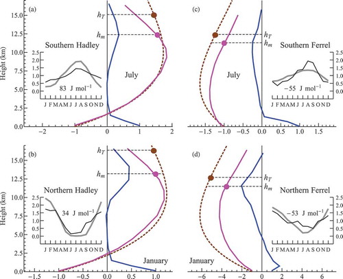
Fig. A2. Annual mean latitudinal profiles of the air temperature lapse rate on different pressure levels in the tropics. Curve 1 in (a) shows the mean lapse rate between 1000 and 925 hPa; curve 11 – between 150 and 100 hPa. Panel (b) shows the relative horizontal variation – at each pressure level the lapse rate at a given latitude is divided by the mean lapse rate at this level (averaged between 30°S and 30°N). The equator has a higher lapse rate than the 30th latitudes in the lower and upper – but not the middle – troposphere. The data are long-term mean NCAR/NCEP climatology (see Appendix D).

We find that both in the Northern and Southern cells the dependence between and changes with growing . While for the smaller values of the relationship in both cells is identical and the proportionality coefficient is about hPa K, it decreases markedly (in the Northern cell reaching zero) with growing (Fig. A3a and b). At constant this results in declining kinetic energy generation [eq. (22)].

Furthermore, while the total surface temperature difference grows with the cumulative extension of the Hadley system, the total surface pressure difference reaches a plateau of 17 hPa for latitude (Fig. A3d and e). Accordingly, for the ratio of cumulative pressure and temperature differences for the Hadley system is essentially constant at around hPa K, but for larger it declines by about one-third as grows up to the maximum observed values (Fig. A3f). For kinetic energy generation declines for latitude. For km becomes zero at the observed maximum extension of the Hadley system, latitude (Fig. A4).

Fig. A3. Relationships between surface temperature and pressure differences and the meridional extension of the Hadley system. (a–c) Dependence of on in (a) Northern Hadley cell, (b) Southern Hadley cell, (c) Hadley system as a whole: , (Fig. 2). (d–f) Dependence of (d), (e) and their ratio (f) on the total extension of the Hadley system () (degrees latitude). Solid lines denote linear regressions for the terciles of , each containing 144 values, for (a, b), (c) and (d–f). Regression parameters are shown in each panel starting from the first tercile.

Fig. A4. Kinetic energy generation at different altitudes in the lower atmosphere versus Hadley system size as determined from eq. (22) using the established relationships between and from Fig. A3d and e.

For our analysis of total kinetic energy generation in the atmosphere, we used NCAR/NCEP monthly re-analyses data provided by the NOAA/OAR/ESRL PSD, Boulder, Colorado, USA, from their website at http://www.esrl.noaa.gov/psd/ (Kalnay et al., 1996). These data include geopotential height and air temperature at 13 pressure levels, sea level pressure and meridional velocity at 1000 hPa on a grid. We averaged the data for each month for the period 1979–2013. Then each variable was zonally averaged producing 73 values for each month for each latitude from 90°S to 90°N. For land the sea level pressure and 1000 hPa air temperature and meridional velocity data are not measurable; the NCAR/NCEP model extrapolations were used (i.e. land areas not excluded).

We defined the cell borders as the grid points where the zonally averaged meridional velocity at 1000 hPa is closest to zero while changing its sign (Fig. A5a). We approximated temperature of the upper streamline (Fig. 3b and Fig. A5c) as the temperature of the top of the troposphere. The latter was defined following Santer et al. (2003) as the height where the vertical temperature lapse rate in the upper atmosphere diminishes to K km. For each latitude, the lapse rate between any two pressure levels was determined as for , where and are the zonally averaged air temperature and geopotential height at pressure level (Fig. A2). If for some in the upper atmosphere , we determined the top of the troposhere assuming locally a linear dependence of lapse rate on .

Fig. A5. Annual mean values of parameters used to calculate global kinetic energy generation. Empty red circles denote cell borders defined in (a) as the points where meridional velocity changes sign. Black circles show temperature and pressure values used in eqs. (27)–(29) (see also Fig. 3b).

In Fig. A1 the observed horizontal pressure differences across the Hadley and Ferrel cells were calculated using the hydrostatic relationship and the chain rule , where is distance along the meridian [see also figure 2e–h of Makarieva et al. (2015c)]. For each cell ( for Hadley, for Ferrel) for . Here is pressure of the th pressure level; and are the latitudes of cell borders closest to the pole and equator, respectively; pressure scale height [see also eq. (26)], g mol, and is the mean air temperature at level .

References

- Bates, J. R. 2012. Climate stability and sensitivity in some simple conceptual models. Clim. Dyn. 38, 455–17. DOI:10.1007/s00382-010-0966-0.
- Bayr, T. and Dommenget, D. 2013. The tropospheric land-sea warming contrast as the driver of tropical sea level pressure changes. J. Climate 26, 1387–1402. DOI:10.1175/JCLI-D-11-00731.1.
- Bony, S., Stevens, B., Frierson, D. M. W., Jakob, C., Kageyama, M. and co-authors. 2015. Clouds, circulation and climate sensitivity. Nat. Geosci. 8, 261–268. DOI:10.1038/ngeo2398.
- Boville, B. A. and Bretherton, C. S. 2003. Heating and kinetic energy dissipation in the NCAR Community Atmosphere Model. J. Climate 16, 3877–3887. DOI:10.1175/1520-0442(2003)016<3877:HAKEDI>2.0.CO;2.
- Cai, M. and Shin, C.-S. 2014. A total flow perspective of atmospheric mass and angular momentum circulations: boreal winter mean state. J. Atmos. Sci. 71, 2244–2263. DOI:10.1175/JAS-D-13-0175.1.
- Chen, G., Held, I. M. and Robinson, W. A. 2007. Sensitivity of the latitude of the surface westerlies to surface friction. J. Atmos. Sci. 64, 2899–2915. DOI:10.1175/JAS3995.1.
- Heffernan, O. 2016. The mystery of the expanding tropics. Nature 530, 20–22. DOI:10.1038/530020a.
- Held, I. M. and Hou, A. Y. 1980. Nonlinear axially symmetric circulations in a nearly inviscid atmosphere. J. Atmos. Sci. 37, 515–533. DOI:10.1175/1520-0469(1980)037<0515:NASCIA>2.0.CO;2.
- Huang, J. and McElroy, M. B. 2014. Contributions of the Hadley and Ferrel circulations to the energetics of the atmosphere over the past 32 years. J. Climate 27, 2656–2666. DOI:10.1175/JCLI-D-13-00538.1.
- Huang, J. and McElroy, M. B. 2015a. Thermodynamic disequilibrium of the atmosphere in the context of global warming. Clim. Dyn. 45, 3513–3525. DOI:10.1007/s00382-015-2553-x.
- Huang, J. and McElroy, M. B. 2015b. A 32-year perspective on the origin of wind energy in a warming climate. Renew. Energy 77, 482–492. DOI:10.1016/j.renene.2014.12.045.
- Johnson, D. R. 1989. The forcing and maintenance of global monsoonal circulations: an isentropic analysis. Adv. Geophysics 31, 43–316.
- Kalnay, E., Kanamitsu, M., Kistler, R., Collins, W., Deaven, D. and co-authors. 1996. The NCEP/NCAR 40-year reanalysis project. Bull. Amer. Meteor. Soc. 77, 437–471. DOI:10.1175/1520-0477(1996)077<0437:TNYRP>2.0.CO;2.
- Kieu, C. 2015. Revisiting dissipative heating in tropical cyclone maximum potential intensity. Quart. J. Roy. Meteorol. Soc. 141, 2497–2504. DOI:10.1002/qj.2534.
- Kim, Y.-H. and Kim, M.-K. 2013. Examination of the global lorenz energy cycle using MERRA and NCEP-reanalysis 2. Clim. Dyn. 40, 1499–1513. DOI:10.1007/s00382-012-1358-4.
- Lindzen, R. S. and Nigam, S. 1987. On the role of sea surface temperature gradients in forcing low-level winds and convergence in the tropics. J. Atmos. Sci. 44, 2418–2436. DOI:10.1175/1520-0469(1987)044<2418:OTROSS>2.0.CO;2.
- Lorenz, E. N. 1967. The Nature and Theory of the General Circulation of the Atmosphere. Geneva: World Meteorological Organization.
- Lorenz, R. D. and Rennó, N. O. 2002. Work output of planetary atmospheric engines: dissipation in clouds and rain. Geophys. Res. Lett. 29, 10-1–10-4. DOI:10.1029/2001GL013771.
- Makarieva, A. M., Gorshkov, V. G., Li, B.-L. and Nobre, A. D. 2010. A critique of some modern applications of the Carnot heat engine concept: the dissipative heat engine cannot exist. Proc. R. Soc. A 466, 1893–1902. DOI:10.1098/rspa.2009.0581.
- Makarieva, A. M., Gorshkov, V. G. and Nefiodov, A. V. 2014. Condensational power of air circulation in the presence of a horizontal temperature gradient. Phys. Lett. A 378, 294–298. DOI:10.1016/j.physleta.2013.11.019.
- Makarieva, A. M., Gorshkov, V. G. and Nefiodov, A. V. 2015a. Empirical evidence for the condensational theory of hurricanes. Phys. Lett. A 379, 2396–2398. DOI:10.1016/j.physleta.2015.07.042.
- Makarieva, A. M., Gorshkov, V. G., Nefiodov, A. V., Sheil, D., Nobre, A. and co-authors. 2015b. Quantifying the global atmospheric power budget. http://arxiv.org/abs/1603.03706.
- Makarieva, A. M., Gorshkov, V. G., Nefiodov, A. V., Sheil, D., Nobre, A. D. and co-authors. 2015c. Comments on “The tropospheric land-sea warming contrast as the driver of tropical sea level pressure changes”. J. Climate 28, 4293–4307. DOI:10.1175/JCLI-D-14-00592.1.
- Makarieva, A. M., Gorshkov, V. G., Sheil, D., Nobre, A. D. and Li, B.-L. 2013. Where do winds come from? A new theory on how water vapor condensation influences atmospheric pressure and dynamics. Atmos. Chem. Phys. 13, 1039–1056. DOI:10.5194/acp-13-1039-2013.
- Marvel, K., Kravitz, B. and Caldeira, K. 2013. Geophysical limits to global wind power. Nat. Clim. Change 3, 118–121. DOI:10.1038/nclimate1683.
- Montgomery, M. T., Bell, M. M., Aberson, S. D. and Black, M. L. 2006. Hurricane Isabel (2003): new insights into the physics of intense storms. Part I: mean vortex structure and maximum intensity estimates. Bull. Amer. Meteor. Soc. 87, 1335–1347. DOI:10.1175/BAMS-87-10-1335.
- Pauluis, O. 2011. Water vapor and mechanical work: A comparison of Carnot and steam cycles. J. Atmos. Sci. 68, 91–102. DOI:10.1175/2010JAS3530.1.
- Pauluis, O., Balaji, V. and Held, I. M. 2000. Frictional dissipation in a precipitating atmosphere. J. Atmos. Sci. 57, 989–994. DOI:10.1175/1520-0469(2000)057<0989:FDIAPA>2.0.CO;2.
- Peixoto, J. P. and Oort, A. H. 1992. Physics of Climate. American Institute of Physics, New York.
- Rienecker, M. M., Suarez, M. J., Gelaro, R., Todling, R., Bacmeister, J. and co-authors. 2011. MERRA: NASA’s modern-era retrospective analysis for research and applications. J. Climate 24, 3624–3648. DOI:10.1175/JCLI-D-11-00015.1.
- Robinson, W. A. 1997. Dissipation dependence of the jet latitude. J. Climate 10, 176–182. DOI:10.1175/1520-0442(1997)010<0176:DDOTJL>2.0.CO;2.
- Santer, B. D., Sausen, R., Wigley, T. M. L., Boyle, J. S., AchutaRao, K. and co-authors. 2003. Behavior of tropopause height and atmospheric temperature in models, reanalyses, and observations: decadal changes. J. Geophysical Research: Atmospheres 108, ACL 1–1–ACL 1–22. DOI:10.1029/2002JD002258.
- Schneider, T. 2006. The general circulation of the atmosphere. Annu. Rev. Earth Planet. Sci. 34, 655–688. DOI:10.1146/annurev.earth.34.031405.125144.
- Schubert, G. and Mitchell, J. L. 2013. Planetary atmospheres as heat engines. In : Comparative Climatology of Terrestrial Planets (eds. S. J. Mackwell, A. A. Simon-Miller, J. W. Harder and M. A. Bullock) University of Arizona Press, Tucson, pp. 181–191. DOI:10.2458/azu_uapress_9780816530595-ch008.
- Shepherd, T. G. 2014. Atmospheric circulation as a source of uncertainty in climate change projections. Nat. Geosci. 7, 703–708. DOI:10.1038/ngeo2253.
- Sobel, A. H. and Neelin, J. D. 2006. The boundary layer contribution to intertropical convergence zones in the quasi-equilibrium tropical circulation model framework. Theor. Comput. Fluid Dyn. 20, 323–350. DOI:10.1007/s00162-006-0033-y.
- Webster, P. J. 2004. The elementary Hadley circulation. In : The Hadley Circulation: Present, Past and Future, Volume 21 of Advances in Global Change Research (eds. H. F. Diaz and R. S. Bradley) Kluwer Academic Publishers, Dordrecht, pp. 9–60
- Wulf, O. R. and Davis, J.,. L. 1952. On the efficiency of the engine driving the atmospheric circulation. J. Meteorol. 9, 79–82. DOI:10.1175/1520-0469(1952)009<0080:OTEOTE>2.0.CO;2.