Lake–atmosphere interactions at Alqueva reservoir: a case study in the summer of 2014

ABSTRACT

The study of lake–atmosphere interactions was the main purpose of a 2014 summer experiment at Alqueva reservoir in Portugal. Near-surface fluxes of momentum, heat and mass [water vapour (H₂O) and carbon dioxide (CO₂)] were obtained with the new Campbell Scientific’s IRGASON Integrated Open-Path CO₂/H₂O Gas Analyser and 3D Sonic Anemometer between 2 June and 2 October. On average, the reservoir was releasing energy in the form of sensible and latent heat flux during the study period. At the end of the 75 d, the total evaporation was estimated as 490.26 mm. A high correlation was found between the latent heat flux and the wind speed (R = 0.97). The temperature gradient between air and water was positive between 12 and 21 UTC, causing a negative sensible heat flux, and negative during the rest of the day, triggering a positive sensible heat flux. The reservoir acted as a sink of atmospheric CO₂ with an average rate of −0.026 mg m⁻² s⁻¹. However, at a daily scale we found an unexpected uptake between 0 and 9 UTC and almost null flux between 13 and 19 UTC. Potential reasons for this result are further discussed. The net radiation was recorded for the same period and water column heat storage was estimated using water temperature profiles. The energy balance closure for the analysed period was 81%. In-water solar spectral downwelling irradiance profiles were measured with a new device allowing measurements independent of the solar zenith angle, which enabled the computation of the attenuation coefficient of light in the water column. The average attenuation coefficient for the photosynthetically active radiation spectral region varied from 0.849 ± 0.025 m⁻¹ on 30 July to 1.459 ± 0.007 m⁻¹ on 25 September.

KEYWORDS:

• lake reservoir
• eddy covariance
• sensible and latent heat fluxes
• energy balance closure
• carbon fluxes
• underwater spectral irradiance profiles
• PAR attenuation coefficient

1. Introduction

Lakes and reservoirs affect the regional climate and are also affected by weather patterns. On the global scale, lakes cover an area of 4.2 million km², corresponding to more than 3% of the Earth’s continental surface (Downing et al., 2006). Despite the small fraction of lakes, these freshwater reservoirs play an important role in mass, energy and momentum exchanges with the atmosphere. The variations in heat and moisture transfers between the inland waters and the atmosphere can influence regional patterns of atmospheric circulation, and thus an effort has been made in recent years to improve the coupling of lake models with weather prediction and climate models (e.g. Balsamo et al., 2012). Furthermore, inland waters can take up carbon dioxide (CO₂) from the atmosphere as well as release CO₂ and methane (CH₄) to the atmosphere, and thus these systems should be taken into account in the carbon cycle (Pacheco et al., 2013). Carbon exchanges between these media occur as a result of physical and biogeochemical processes (Wetzel, 1983). More accurate estimation of greenhouse gas exchanges between inland water bodies and the atmosphere has become of increasing concern in recent years (Cole et al., 2007). The eddy covariance (EC) method is the most common technique used to assess turbulent fluxes over all types of surfaces (Baldocchi, 2003). The EC method is a non-invasive technique, normally installed in a tower, with less impact on the environment compared to the use of chambers (Repo et al., 2007). These turbulent fluxes, obtained with direct and continuous measurements, are important to estimate the exchanges of energy, water and greenhouse gases between the surface and the atmosphere. This technique has also been used to estimate CO₂ and CH₄ fluxes over aquatic environments (e.g. Vesala et al., 2012; Podgrajsek et al., 2014; Mammarella et al., 2015). In 2014, a set of EC measurements was carried out at a Portuguese reservoir to estimate the CO₂, H₂O, heat and momentum fluxes over water, within the framework of the ALEX project (www.alex2014.cge.uevora.pt). During 4 months, continuous measurements were carried out on a floating platform in the Alqueva reservoir, located in the south-east of Portugal. This field campaign gave continuity to previous studies (e.g. Salgado and Le Moigne, 2010; Le Moigne et al., 2013) performed in Alqueva reservoir in the summer of 2007 and in Thau Lagoon in the summer of 2011, with the objectives of understanding mass, energy and momentum exchanges between the atmosphere and reservoirs.

The effect of climate variability on the reservoir thermal structure, water quality and aquatic ecosystems has long been known to be important (Nowlin et al., 2004; Lee and Biggs, 2014; McGloin et al., 2014). To understand the role of lakes on weather and climate, fully coupled models must be improved in which key lacustrine processes have to be represented. The aquatic photosynthesis processes occur in the euphotic zone, the layer between the surface and the depth of 1% of the subsurface irradiance, and this layer can be thicker in clear waters and thinner in turbid ones (Bukata et al., 1995; Wozniak et al., 2003). Some instrumentation has been developed to measure the underwater radiance field in lakes, fjords and oceans (Sasaki et al., 1958; Jerlov and Fukuda, 1960; Tyler, 1960; Lewis et al., 2011; Antoine et al., 2013; Potes et al., 2013). In particular, Potes et al. (2013) developed a new apparatus to be coupled with a portable spectroradiometer, allowing for spectral radiance measurements in underwater environments and to subsequently obtain estimates of the spectral and broadband light attenuation coefficients in water. The light attenuation coefficient is relevant in the water surface layer energy budget. In particular, it is an important parameter in lake models for computing the water surface temperature, which is used for estimating heat and moisture transfers between water bodies and the atmosphere (Mironov et al., 2010; Potes et al., 2012). Nevertheless, the use of measurements of hemispherical spectral radiance (irradiance) is preferable to obtain more reliable attenuation coefficients. Such irradiance measurements are scarce, but they have been performed in the Mediterranean Sea with moored radiometers at fixed levels below the surface (Gernez and Antoine, 2009), in field experiments in the Irish Sea and open ocean (Bowers and Mitchelson-Jacob, 1996; Darecki et al., 2011), and in lakes and reservoirs (Liu et al., 2010; Heiskanen et al., 2015). In this way, and within the framework of the above-mentioned ALEX project, sporadic measurements of underwater downwelling spectral irradiance were performed during the 4 month study with the new equipment.

In Sections 2 and 3, respectively, the study site and the instrumental set-up are introduced. The results obtained are discussed in Section 4, where a detailed analysis of the heat fluxes, energy balance and CO₂ flux is presented, followed by a detailed examination of the spectral underwater solar irradiance profiles and the resulting estimate of the spectral attenuation. A first study of observational evidence of lake breeze induction at Alqueva reservoir is presented at the end of this section. In Section 5, the main conclusions are summarized.

2. Study site

The Alqueva reservoir is located in the south-east of Portugal along 83 km of the main course of the Guadiana River, where the northern branch is shared with Spain (Fig. 1). The reservoir has maximum and average depths of 92.0 m and 16.6 m, respectively. It has a total capacity of 4150 km³ and a surface area of 250 km², and constitutes the largest artificial lake in the Iberian Peninsula. The reservoir is used for water supply, irrigation and hydroelectric power generation. Water samples taken at the euphotic zone in Alqueva-Montante platform (Fig. 1) to evaluate the trophic status of the water indicate a mesotrophic status based on chlorophyll a as an indicator of phytoplankton productivity.

Fig. 1. Alqueva reservoir: geographic location, floating platforms and meteorological stations. A zoom from Alqueva-Montante platform equipped with the IRGASON instrument; details of the sonic anemometer, gas analyser and accelerometer.

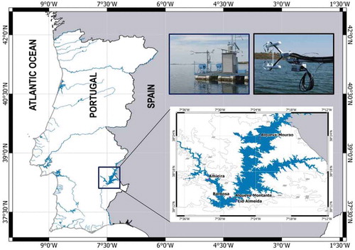
The reservoir was established in 2002 in a region long known for the irregularity of its hydrological resources, with periods of drought that may last for more than one consecutive year (Silva et al., 2014), and it is classified as a Csa region according to the Köppen climate classification. This class corresponds to temperate climates with dry and hot summers (Mediterranean climate). The rainfall period occurs seasonally between October and April, with an average annual precipitation of 558 mm, as recorded in Beja (about 40 km from the reservoir) for the period 1981–2010 (www.ipma.pt). The summer synoptic circulations over the region are strongly constrained by the location and shape of the Azores anticyclone and by the frequent establishment of a thermal low over the Iberian Peninsula, induced by the land–ocean thermal contrasts. Under the sea breeze system, organized at the peninsular scale by the thermal low, the maritime air mass penetrates towards the interior of the peninsula. The breeze originating on the west coast has been documented to reach more than 100 km inland, reaching the region in the late afternoon, as evident from the increase in wind intensity and its rotation (Salgado et al., 2015). The summer Local Time (LT) in Portugal has the following relation with UTC: LT = UTC + 1.

3. Instrumental set-up and methods

3.1. Eddy covariance system and other supporting measurements

This field campaign study was performed in the Alqueva reservoir area, implementing an appropriate experimental set-up, between 2 June and 2 October 2014 (Fig. 1). Three meteorological stations were established over land near the reservoir shore: Amieira (38º 16ʹ 39.18ʹʹ N, 7º 32ʹ 2.10ʹʹ W), Barbosa (38º 13ʹ 39.18ʹʹ N, 7º 28ʹ 14.74ʹʹ W) and Cid Almeida (38º 12ʹ 59.00ʹʹ N, 7º 27ʹ 16.34ʹʹ W). Two floating platforms were equipped over water: Alqueva-Montante (38º 13ʹ 24.75ʹʹ N, 7º 27ʹ 34.18ʹʹ W) and Alqueva-Mourão (38° 23ʹ 37.08ʹʹ N, 7° 23ʹ 15.18ʹʹ W). The depths at Alqueva-Montante and Alqueva-Mourão are 65 m and 48 m, respectively.

The terrestrial stations measure air and soil temperature, relative humidity, wind speed and direction, and precipitation. Both floating platform stations measure water temperature profile, air temperature, and wind speed and direction. In addition, the instrumentation installed in Alqueva-Montante platform comprises: one EC system at 2 m above the water surface, the Integrated Open-Path CO₂/H₂O Gas Analyser and 3D Sonic Anemometer (IRGASON; Campbell Scientific); one albedometer (CM7B; Kipp&Zonen) for short-wave radiation measurements; one pyrradiometer (8111; Philipp Schenk) for long-wave radiative balances and nine temperature probes (107; Campbell Scientific) at several depths (0.05, 0.5, 1.0, 2.0, 3.0, 6.0, 9.0, 18.0 and 27.0 m).

Variables measured by IRGASON were u, v and w components of wind speed, sonic temperature, H₂O and CO₂ concentration, and sonic anemometer and gas analyser quality flags. Data were sampled at 20 Hz and the filter time delay was 200 ms.

In addition, occasional measurements of water temperature, turbidity, pH, dissolved oxygen and conductivity in the water column were taken with a multiparameter probe (In-Situ TROLL 9500 Profiler XP) nearly twice a month.

3.2. Eddy covariance flux calculation

Turbulent fluxes of momentum, heat and mass (H₂O and CO₂) were calculated as 30 min covariances between fluctuations of vertical wind component w and temperature, H₂O and CO₂ concentration, respectively. Before covariance calculation, the turbulent time series were linearly detrended (Rannik and Vesala, 1999) and double-axis rotation was applied to the wind speed components (Rebmann et al., 2012). Furthermore, two necessary corrections were applied to the flux calculations: the first one concerns the H₂O and CO₂ fluxes, and accounts for the air density fluctuations due to thermal expansion and water vapour dilution (Webb et al., 1980); the second is the humidity correction of sonic temperature according to Kaimal and Gaynor (1991). The corrected turbulent fluxes of momentum (τ, kg m⁻¹ s⁻²), sensible heat (H, W m⁻²), latent heat (LE, W m⁻²) and CO₂ (F_c, mg m⁻² s⁻¹) were obtained as follows (positive when upward):

(1)

(2)

(3)

(4)

where is the air density (kg m⁻³); is the water vapour density (kg m⁻³); is the density of dry air (kg m⁻³); is the gas constant for dry air (kPa m³ K⁻¹ g⁻¹); R is the universal gas constant (8.3143 × 10^–3 kPa m³ K⁻¹ mol⁻¹); is the ambient pressure (kPa); is the ratio of the molecular weight of dry air to water vapour; is the temperature corrected for water vapour (K): ; is the sonic temperature in air (K); is the specific heat of air (J kg⁻¹ K⁻¹); is the gas constant for water vapour (kPa m³ K⁻¹ g⁻¹); is the latent heat of vaporization (J kg⁻¹); and is CO₂ density (mg m⁻³).

The footprint analysis was done according to Kljun et al. (2004), for 90% contribution (X₉₀, m) and peak contribution (X_max, m) distances:

(5)

(6)

where is the standard deviation of the vertical velocity fluctuation (m s⁻¹); is the friction velocity (m s⁻¹); is the sensor height (m); and and are parameters that depend on the roughness length (z₀, m). In this work, z₀ was computed according to Ferdorovich et al. (1991):

(7a)

(7b)

where is the air viscosity; and .

The atmospheric stability parameter () was calculated using the Obukhov length (L, m):

(8)

where is the von Karman constant.

3.2.1. Data quality criteria and filters applied

IRGASON provides diagnostic flags for the sonic anemometer and gas analyser. With these diagnostic flags, the data set was filtered for bad data or measurement problems of the sonic anemometer and gas analyser. The gas analyser provides the CO₂ and H₂O signal strength, which is an indicator of data quality, and ranges between 0.0 (not working or optical path obstructed) and 1.0 (working perfectly). Data with signal strength lower than 0.7 are discarded owing to poor quality. The fluxes are validated according the wind direction to avoid contamination of the measurements by the platform; thus, wind directions between the angles of 90º and 270º were discarded from the data set (see details in Section 4.1). Footprints (fetch) with values of X₉₀ greater than 300 m were also discarded to ensure exclusively water body contributions to the measurements. In summary, about 37% of the data were discarded as a result of the criteria and applied filters described above.

3.3. Energy balance

The energy balance closure (EBC) and the energy residual (Res) of the lake can be obtained using the latent (LE) and the sensible (H) heat fluxes, the net radiation (Rn) and the water column heat storage (), assuming horizontal homogeneity and neglecting the heat fluxes due to precipitation, runoff and bottom sediments, through eqs (9) and (10):

(9)

(10)

The water column heat storage () is computed using eq. (11):

(11)

where is the water density, calculated as a function of depth-weighted average temperature according to Gill (1982); and is the specific heat of water (4192 J kg⁻¹ K⁻¹). Since the continuous temperature profiles were available only to a depth of 27 m, the water temperature to the bottom was obtained through linear extrapolation using data from the multiparameter probe profiles (see Section 3.1). The error of these extrapolations should be small as the water temperature below 27 m has a small variation to the bottom, i.e. during this 4 months ΔT between 27 and 65 ms varied from 1.14 ºC in June to 3.42 ºC in September.

3.4. Underwater spectral irradiance field

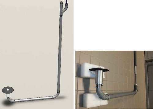
In the study of Potes et al. (2013), the downwelling radiance measurements were carried out with an optical device fully described in this reference. Because of its small field of view (FOV = 22º), some problems were found under small solar zenith angles, e.g. when the water upper layers were exposed to the penetration of direct zenith sunlight due to the refraction on the surface and to light scattering (Potes et al., 2013). Thus, the need to have measurements that are independent of the solar zenith angle motivated the development of a new tip to measure the hemispherical radiance (180º), enabling the calculation of the attenuation coefficient from the subsurface level down to 3 m depth (see Fig. 2 for details). This new receiver, a Metcon GmbH brand, consists of an optical input system designed to collect incoming radiance from all directions of a hemisphere. The receiver is tuned by the manufacturer to achieve uniform transfer function on the 2π sr. The test measurements performed in the laboratory, with a collimated beam irradiating the device at ± 90° with respect to its longitudinal axis, confirmed the data provided by Metcon. This kind of device has already been used for the estimation of J values for atmospheric compounds and has been fully described previously (Kostadinov et al., 2003, 2009). This new receiver is attached to an apparatus similar to that described in the work of Potes et al. (2013) and is composed of a portable spectroradiometer, linked to an optical fibre bundle driven by a customized frame for protection and to keep the tip pointing to the zenith direction in the underwater environment. The portable FieldSpec UV/VNIR Spectroradiometer (Analytical Spectral Devices; Boulder, CO, USA) was used to record the spectral downwelling zenith irradiance measured across the spectral range 325–1075 nm with a spectral resolution ranging from 1 to 3 nm for the ultraviolet (UV) and near-infrared (NIR) spectral regions, respectively. The fibre bundle was chosen to meet the optical features of the spectroradiometer and the core is made of quartz, allowing measurements in the UV spectral region as well. To maximize the signal reaching the spectrometer, the packing factor of the bundle was optimized, using single fibres with the same numerical aperture but with different diameters: 0.11 and 0.22 mm. The frame was developed to guarantee the verticality and horizontality of the bare tip of the fibre bundle, which has to point upwards to the zenith to collect the downwelling zenith radiance at several levels below the water surface. Before every profile measurement, the integration time of the spectroradiometer was optimized to ensure the best illuminating conditions. Also, a dark current spectrum (which is an offset that varies with the temperature of the detector) was taken before every profile to correct the signal for temperature oscillations. A sample average of 10 spectra and three samples were taken per level. This choice was made to compromise between a preferentially high number of spectra per level and a relatively fast profiling under almost the same atmospheric conditions. This version was tested in a 5 m deep pool from the municipal swimming complex of Évora. After the test sessions, the apparatus was used to perform measurements in Alqueva reservoir in the summer of 2014, during the ALEX2014 field campaign. All underwater irradiance measurements during the campaigns were taken under clear sky conditions. The length of the fibre bundle allows for measurements to a maximum depth of 3 m and the levels chosen for the profiles were: above water surface, 0.01, 0.05, 0.25, 0.50, 0.75, 1.00, 1.50, 2.00, 2.50 and 3.00 m. These profiles allow for the calculation of the spectral attenuation coefficient () of the water column, using the equation presented by Preisendorfer (1959):

(12)

Fig. 2. Scheme of the apparatus developed for measurements of spectral underwater solar irradiance. Detail of the optical receiver and multilayer protecting frame of underwater device for measuring downwelling spectral irradiance.

where E is irradiance, is the depth, is the solar zenith angle, is the solar azimuth angle, and is the wavelength.

In the case of our measurements, the depth (in eq. 12) is replaced with depth , which is the depth of the layer where the logarithmic slope of the underwater radiance becomes nearly constant with depth (eq. 5 in Potes et al., 2013).

4. Results and discussions

4.1. Flux data quality, footprint and atmospheric stability

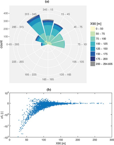
Regarding the EC system installed in the floating platform (Fig. 1), some quality analysis need to be done for operational control of the system. Co-spectral analysis is normally used to evaluate the frequency response of the analyser (Kaimal et al., 1972; Nordbo et al., 2011; Mammarella et al., 2015). Comparison between actual co-spectra shapes and ideal ones obtained from models is generally a good method of evaluation. As an example, Fig. 3 shows the average normalized frequency-weighted co-spectra as a function of normalized frequency for temperature, CO₂ and water vapour for the period 23–26 July 2014. The three co-spectra are in accordance with the expected ideal curve; for higher frequencies, the slopes tend to the value of n^−4/3 (Kaimal et al., 1972), with peaks at frequencies around n = 0.05. Since no damping is present at high frequencies, there is no need for frequency response correction. In Fig. 4a, the X₉₀ distribution is shown for the accepted wind sector. The average values of the footprint are 106.8 m and 53.2 m for X₉₀ and X_max, respectively (the latter not shown here). With maximum values of around 300 m for X₉₀, it can be ensured that the footprint refers to the water surface and there is no contamination from the shores or land in the measurements. Figure 4b shows how the footprint (X₉₀) depends on the atmospheric stability. It is also clearly visible that unstable stratification (z/L < 0) corresponds frequently to calm wind conditions (low friction velocity) and lower footprints. In contrast, near-neutral stratification (z/L close to zero) corresponds to stronger wind (high friction velocities) and higher values of X₉₀. Under stable conditions, Fig. 4b shows some unusual cases of low X₉₀, probably due to the existence of local stability, during the afternoon, induced by the contact with colder water (high z/L and low σ_w) under a prevailing larger scale boundary layer circulation of unstable air (low friction velocity).

Fig. 3. Average normalized frequency-weighted co-spectra for CO₂, H₂O and sonic temperature (T_s) as a function of normalized frequency for the period 23–26 July 2014.

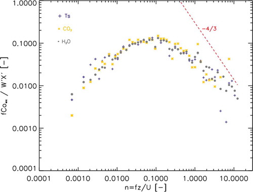
Fig. 4. (a) Footprint length (X₉₀) in the wind directions 270–90º; (b) scatterplot of footprint (X₉₀) and stability (z/L) during the period June–September 2014.

4.2. Heat fluxes and energy balance

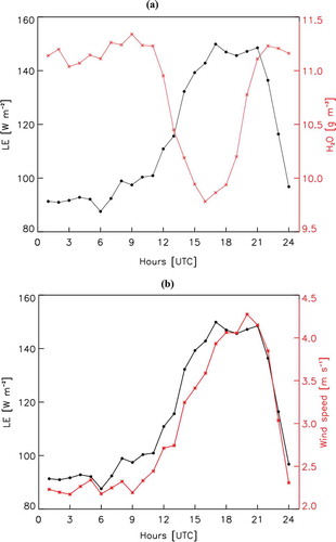
The mean daily cycle of H and the difference between air temperature (2.0 m) and near-surface water temperature (0.05 m) are shown in Fig. 5. It is clear that when the temperature difference is negative, H is positive, with a maximum of 31.34 W m⁻² at 7 UTC. During the afternoon, when the air temperature over the reservoir is higher than the water skin temperature, a slightly stable internal boundary layer develops, leading to a negative H, with a minimum of −18.09 W m⁻² at 18 UTC (Fig. 5). In the same period, the water vapour content minimum (9.78 g m⁻³ at 16 UTC) (Fig. 6a) occurs, partially related to the development of a lake breeze (discussed in Section 4.5). As seen in Fig. 6b, LE is highly correlated with the wind speed (R = 0.97). Wind speed strongly increases between 13 and 18 UTC, and reaches a maximum at 20 UTC (4.17 m s⁻¹), corresponding to the arrival of the sea breeze which originated on the west coast (Salgado et al., 2015). LE has a first and higher maximum of 148.83 W m⁻² at 17 UTC and a second maximum at 21 UTC. These results are in agreement with a previous study by Salgado and Le Moigne (2010) for the same reservoir, showing an absolute maximum of LE at 21 UTC and also a change of sign in H according to the sign of the air–water temperature difference. Considering that the reservoir presents a homogeneous surface, it is estimated that 19.45 GJ of energy was released in the form of H and 490.26 mm of water was lost in the form of evaporation during the 4 month period of study. In contrast, the total precipitation in the same period was 74 mm, with 75% occurring in September.

Fig. 5. Mean daily cycle of sensible heat flux (left y-axis; circles) and temperature difference between air (2 m) and near-surface water (right y-axis; stars) during the period June–September 2014.

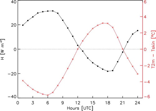
Fig. 6. (a) Mean daily cycle of latent heat flux (LE) (left y-axis; circles) and water vapour (right y-axis; stars); (b) mean daily cycle of latent heat flux (left y-axis; circles) and wind speed (right y-axis; stars), during the period June–September 2014.

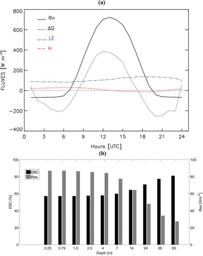
The average diurnal cycle of LE and H, the net radiation (Rn) and the water column heat storage () over the entire period are plotted in Fig. 7a. In this case, the plotted was computed considering only 4 m depth, which is the depth that best represents the daily cycle, because, at the daily scale, small errors in deep-layer temperature measurements rise to large errors on estimation. Rn makes a major contribution, with an average value of 201.97 W m⁻², and part of this energy is used to heat up the first 4 m depth of the reservoir, resulting in an average value of 2.68 W m⁻² to . The sum of H and LE is, on average, 115.37 W m⁻². The energy balance closure (EBC) and the residual energy (Res) of the lake were estimated using eqs (9) and (10). was estimated for different depths of the reservoir, e.g. 0.25, 4, 7, 14, 24, 38 and 65 m (Fig. 7b). For example, considering the 4 m depth discussed above, the EBC and Res values are 58% and 83.92 W m⁻². Better results are found with the depth of the reservoir in Alqueva-Montante platform (65 m), with values of 81% for EBC and 27.10 W m⁻² for Res. This value of EBC is comparable to those found for two lakes in Finland by Nordbo et al. (2011), with average values of 82% and 73% for 2006 and 2007, and Mammarella et al. (2015), with average values of 83% and 79% for 2010 and 2011.

Fig. 7. (a) Mean daily cycle of net radiation (Rn), water column heat storage (∆Q), latent heat flux (LE) and sensible heat flux (H) during the period June–September 2014. (b) Average energy residual (Res) measured with different depths for water column heat storage (∆Q) calculations during the period June–September 2014. EBC = energy balance closure.

4.3. Carbon dioxide flux

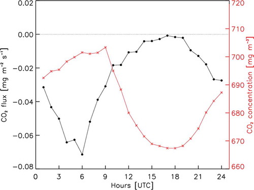
The diurnal curves of atmospheric CO₂ concentration and flux, averaged over the 4 month period, are shown in Fig. 8. It can be noted that the CO₂ flux is negative during the day, more negative during the night and early morning, and nearly zero in the afternoon. The CO₂ concentration shows the opposite behaviour, with higher values during the night and early morning, and lower values in the afternoon, which is typically due to inland plant respiration throughout the night-time and plant photosynthesis during daytime. Higher CO₂ atmospheric concentrations may induce a gradient of CO₂ partial pressure between the near-surface atmosphere and the lake during the night and morning, which can explain a negative flux. During the afternoon, it seems that the gradient is smaller and an almost null CO₂ flux is observed.

Fig. 8. Mean daily cycle of CO₂ flux (left y-axis; circles) and CO₂ concentration (right y-axis; stars) during the period June–September 2014.

There are no measurements of dissolved CO₂ concentrations in the water available for this study; nevertheless, it is well known that the solubility of CO₂ decreases with increasing temperature (Wetzel, 1983), whereby during the night, low water temperature favours CO₂ uptake. Applying Van’t Hoff equations to Henry’s solubility, it is possible to estimate the temperature dependence for Henry’s constant (Sander, 2015): , where is Henry’s constant, is the enthalpy of dissolution, and R is the universal gas constant. For example, for a 5 ºC decrease in water temperature (from 27 ºC to 22 ºC), Henry’s constant will increase by 12.6%.

Furthermore, when absorbed CO₂ reacts with water molecules, it results in the production of carbonic acid (). Carbonic acid dissociates rapidly, relative to the hydration reaction (above mentioned), in bicarbonate () and carbonate ions (), which in turn react with water, forming hydroxyl ions (), and consequently decrease the pH of water. The increase in water acidity is thus an indicator of CO₂ absorption by water. Unfortunately, there were no continuous pH measurements during the period under study. However, continuous measurements performed in previous years (data available at http://snirh.pt), at the same place, indicate the existence of a daily pH cycle (not shown here), with lower values during the night and morning, suggesting that during summer nights the reservoir acts as a sink of CO₂.

Sporadic measurements of water pH were performed during the field campaign and the values at the surface ranged between 8.9 in June and 9.6 in August. With these values of pH, bicarbonate () is assumed to be the dominant species of the three major inorganic carbons ( present in water, with a relative percentage around 90%, while free CO₂ dominates with pH values of 5 (Emerson, 1975; Margalef, 1983; Wetzel, 1983). It was observed by Finlay et al. (2009) and Tranvik et al. (2009) that lakes with pH above 8.0 and 8.6, respectively, act as sinks of atmospheric carbon. Nevertheless, according to Helbig et al. (2016), a systematic bias was found in the CO₂ fluxes during a comparison study between two Campbell Scientific open-path sensors (Irgason and EC150) and two closed-path sensors (EC155 from Campbell Scientific and LI-7200 from LI-COR Biosciences). This bias is related to the so-called spectroscopic effect, and it is more evident when CO₂ fluxes are low and kinematic temperature fluxes are high (sensible heat flux). According to the same authors, the fast-response sonic temperature (instead of slow-response air temperature) should be used in the absorption-to-CO₂ density conversion, which cannot be done in our study since the raw absorption was not recorded during the field campaign. In our case, the period with low CO₂ flux and high sensible heat flux corresponds to night-time (see Figs 5 and 8) and thus the night-time CO₂ uptake by the reservoir may be, in reality, less pronounced than the one calculated in this study. Note that the mean values are always negative but very close to zero between 15 and 19 UTC, with values of the order of 10^–3 and 10^–4 mg m⁻² s⁻¹. The minimum mean value is reached at 6 UTC, −0.071 mg m⁻² s⁻¹, with an absolute minimum of −0.410 mg m⁻² s⁻¹ registered at the same time. During the night and morning, greater carbon uptake by the lake agrees with greater instability in the internal boundary layer (described in subsection 7.1 from Brutsaert, 1982), formed above water, since the water surface is warmer than the air (Fig. 5). It is also during the night that convective instability occurs in the water column, when the water surface temperature decreases and is slightly lower than that of the layers below (not shown), allowing unsaturated water to reach the surface. On the other hand, during the afternoon and under near-surface stability conditions (water being cooler than air), the mean values approach zero, indicating almost null transfer of carbon between the reservoir and the atmosphere. During this period, the water surface is much warmer than the layers below and thus no convection develops. The results discussed above were also found by Lee et al. (2014) at Lake Taihu in south-eastern China. This very large and eutrophic lake (2400 km²) also presented a nocturnal uptake of CO₂ and during this period they found convective instability in the water column.

Considering the whole 4 month period, the average CO₂ flux was −0.026085 mg m⁻² s⁻¹, with an average of −0.043683 mg m⁻² s⁻¹ between 0 and 12 UTC and −0.010700 mg m⁻² s⁻¹ between 12 and 24 UTC. Assuming this flux rate over 1 yr, the value of −13.71 g C m⁻² yr⁻¹ is comparable to the estimations obtained for other lakes and reservoirs described in Pacheco et al. (2013).

Nevertheless, this result represents only 4 months of the year (June to September) and uncertainties remain, especially because of the systematic bias of the IRGASON system, which at the moment is only partially understood (Helbig et al., 2016). Therefore, further long-term studies are necessary to fully characterize the annual carbon cycle in Alqueva reservoir.

4.4. Underwater solar irradiation and spectral attenuation coefficient

The vertical structure of the underwater radiative absorption plays an important role in the thermal dynamics of the water surface layer and consequently on the energy budget at the water–lake interface. So, a better estimation of the irradiance at different levels is relevant to understand the lake–air interactions. Figure 9 presents the profiles of the underwater downwelling irradiance measured with the new device, performed at 10:24 UTC (Fig. 9a), and the underwater downwelling radiance with the device from Potes et al. (2013), performed at 10:52 UTC. The profiles were obtained on 10 July 2014 in Alqueva-Montante (Fig. 1). It can be seen that the new device recorded a decrease in irradiance with depth (Fig. 9a), while the previous device recorded an increase in radiance from the surface to 1 m depth (Fig. 9b). This particular intensification of radiance is associated with the incidence of refracted direct and scattered solar radiation into the FOV cone (Potes et al., 2013). The average attenuation coefficient for the photosynthetically active radiation (PAR) spectral region was computed according to eq. (12) for both profiles. The attenuation coefficient with the new device was 0.709 ± 0.006 m⁻¹ for the layer 0–3 m and with the previous device was 0.522 ± 0.017 m⁻¹ for the layer 1–3 m, which is the layer where the logarithmic slope of the underwater radiance becomes nearly constant with depth (Potes et al., 2013). This comparison confirms that previous estimations of the attenuation coefficient obtained with the Potes et al. (2013) apparatus are comparable to those obtained with the new device; however, it tends to underestimate the coefficient and has a greater degree of uncertainty.

Fig. 9. Profiles in Alqueva-Montante on 10 July 2014: (a) underwater downwelling spectral irradiance measured with the new devices; (b) underwater downwelling spectral radiance with the device from Potes et al. (2013). Profiles are given in digital numbers (DN); output values without calibration.

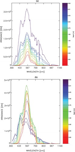
Figure 10 shows two profiles of the downwelling irradiance performed at the pool on 14 July 2014 at 10:32 UTC (Fig. 10a) and at Alqueva-Montante on 27 August 2014 at 10:25 UTC (Fig. 10b). These two profiles present similar spectral behaviour in the 700–900 nm spectral region, where both types of water absorb the radiation. Nevertheless, large differences are noticed in the PAR region. In the pool (Fig. 10a), the solar radiation penetrates more deeply in the range 400–500 nm, with a maximum of 70% of the subsurface irradiance at 3 m depth, while at Alqueva (Fig. 10b) only a maximum of 10% is recorded at 3 m depth, in the 500–600 nm spectral region. At 3 m depth in the pool, there is more than 50% of surface irradiance between 400 and 600 nm. At the same depth in the reservoir, there is only 1–10% between 500 and 700 nm. This indicates that in the reservoir the euphotic depth is reached (for almost all the wavelengths) within the 3 m profile. Figure 11 shows a plot of the spectral attenuation coefficient for the sporadic measurements performed during the field campaign (details are given in Table 1). The spectra from the municipal swimming complex are closer to pure water (Smith and Baker, 1981) from 600 to 800 nm and higher from 325 to 600 nm. The reservoir spectra are higher than pure water and swimming complex, and the minimum shifts from the blue region to the green region of the spectrum. This is due to different composition of the water masses in terms of organic and inorganic material, especially chlorophyll a and cyanobacteria concentration and water turbidity (Morais et al., 2007; Potes et al., 2011, 2012).

Table 1. Measurement details

Date	Time (UTC)	Measurement location	PAR attenuation coefficient^a (m^−1)
Smith and Baker (1981)	–	Pure water	0.166
10 July 2014	10:24	Alqueva-Montante	0.709 ± 0.006
14 July 2014	10:32	Swimming complex	0.191 ± 0.002
30 July 2014	11:19	Alqueva-Montante	0.849 ± 0.025
27 August 2014	10:25	Alqueva-Montante	0.875 ± 0.023
27 August 2014	14:30	Alqueva-Mourão	1.112 ± 0.019
25 September 2014	15:31	Alqueva-Montante	1.055 ± 0.004
25 September 2014	10:39	Alqueva-Mourão	1.459 ± 0.007

^aPhotosynthetically active radiation attenuation coefficient for the layer 0–3 m.

Fig. 10. Profiles of underwater downwelling spectral irradiance: (a) in the municipal swimming complex of Évora; (b) in Alqueva reservoir. Profiles are in percentage of surface irradiance.

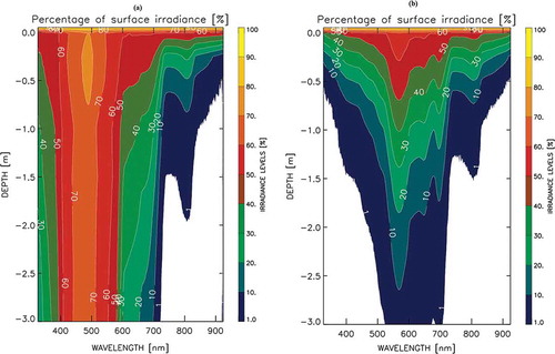
Fig. 11. Spectral attenuation coefficient for the field campaigns described in Table 1.

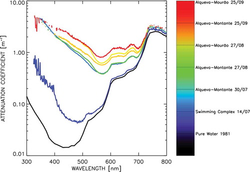
The average attenuation coefficient for the PAR region was computed according to eq. (12). The PAR attenuation coefficients of the most significant profiles obtained in the campaign are shown in Table 1. This spectral region concentrates about half of the solar radiation, and thus the radiation is able to penetrate more deeply in the PAR region than outside it (Fig. 10). Therefore, most of the water quality studies on lakes and lagoons focus on the PAR spectral region (Walmsley et al., 1980; Gallegos, 2001; Potes et al., 2012). Notice that the measurements performed on the same day and at different sites of the reservoir present considerable differences in the PAR attenuation coefficient (Table 1). For example, on 25 September 2014 the difference between the sites Alqueva-Mourão and Alqueva-Montante was about 0.404 m⁻¹, which is more than the double that with respect to the swimming complex water.

4.5. Lake breeze on selected days

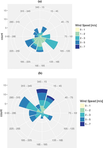
Differences in the surface energy budget between lake–atmosphere and land–atmosphere interfaces create heterogeneities in the air temperature and pressure fields that may induce the formation of local breezes. As the first study of observational evidence of breeze induction at Alqueva reservoir, it was decided to pay special attention to those days on which the effects of the lake on the atmosphere are expected to be more pronounced. The criteria for the selection were: the daily maximum of the temperature difference between air (in Barbosa station) and water (in Alqueva-Montante) was greater than 7 ºC (on average, this temperature difference was 8.17 ºC); and the daily average wind speed was lower than 3.5 m s⁻¹ at Barbosa station. The application of these criteria resulted in the selection of 23 days. With these criteria, the selected days correspond to clear situations of lake breeze, avoiding the presence of a strong synoptic circulation or a strong sea breeze, which can mask the local effects. On these 23 selected days, a relatively strong lake breeze was found, comparing the measurements in three stations located on the lake shore: Amieira, Barbosa and Cid Almeida (see Fig. 1). Wind direction for the period 13–15 UTC is presented in Fig. 12 for Barbosa and Cid Almeida stations (1 min resolution), the first located on the north-western shore of the reservoir and the second on the south-eastern shore, at a distance of 1900 m from Barbosa station (see Fig. 1 for details). In the period considered (13–15 UTC, when the breeze is stronger), high percentages (65.15% and 79.54%) of wind blowing from the lake to the shore (from the south quadrant in this case) were found for the stations located on the northern shore, Amieira (not shown here) and Barbosa, respectively. For the same period, at Cid Almeida station, located on the south-eastern shore, 54.09% of the winds blew from the north quadrant, again from a lake-to-shore direction.

Fig. 12. Wind rose for 23 selected days in the period 13–15 UTC (units of m s⁻¹) for (a) Barbosa and (b) Cid Almeida stations (1 min resolution). The criteria for the selection were: daily maximum of the temperature difference between air (in Barbosa station) and water (in Alqueva-Montante) greater than 7 ºC, and daily average wind speed lower than 3.5 m s⁻¹ at Barbosa station.

For the period 9–18 UTC, the wind changed from the north component to the south component at Barbosa station, which is located on the northern shore of the reservoir. In Cid Almeida station, located on the southern shore of the reservoir, the wind remained from the north quadrant during that period (not shown here). In terms of intensity and duration, 22 July 2014 was the day with the strongest lake breeze, recorded roughly from 9 to 18 UTC, with average wind velocities of 0.97 and 2.75 m s⁻¹ in Barbosa and Cid Almeida, respectively. These values are slightly higher than the wind velocities before the lake breeze formation (values from 7–9 UTC: 0.72 and 2.40 m s⁻¹ in Barbosa and Cid Almeida, respectively). The effect of the lake breeze, developed in Alqueva reservoir, on LE was explored. The daily cycle of LE flux averaged over the 23 lake breeze days is plotted in Fig. 13 together with the cycle for the 27 no lake breeze days. Those days without lake breeze were defined as days with a daily average temperature difference between air (in Barbosa station) and water (in Alqueva-Montante) lower than 2 ºC. On average, this temperature difference was −0.87 ºC. In the presence of a lake breeze, the latent heat flux was lower than in the cases when the breeze was absent, with average values of 93.45 and 133.58 W m⁻², respectively. In Fig. 13, a decrease in latent heat flux between 9 and 17 UTC is visible for the days with lake breeze overlapping the period of lake breeze. During lake breeze events, the maximum latent heat flux occurs at 22 UTC, with a much smaller value (145.20 W m⁻²) than in the absence of lake breeze, 172.91 W m⁻² at 17 UTC.

Fig. 13. Mean daily cycle of latent heat flux for 23 selected days with development of lake breeze and 27 selected days without lake breeze.

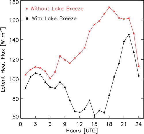
The days when a lake breeze develops are characterized by weak, large-scale winds in the low troposphere. On the other hand, in a lake breeze situation there is air subsidence over the centre of the lake (the descending branch of the thermal circulation) limiting the vertical fluxes. These two features, low near-surface winds (shown for all periods in Fig. 6b) and subsidence, contribute towards reducing the evaporation of the lake.

5. Conclusion

Measurements of energy and mass (H₂O and CO₂) fluxes were continuously performed from June to September 2014 at a floating platform in Alqueva reservoir, south-east of Portugal, with a Mediterranean climate (Csa according to the Köppen classification). During this period, the temperature gradient between the atmosphere and reservoir presents two opposite behaviours during the daily cycle. A positive gradient is observed during the afternoon; thus, a negative sensible heat flux is detected in the afternoon and, consequently, slightly stable atmospheric conditions near the water surface are noticed in this period. The wind speed presents a peak later in the afternoon owing to the arrival of the sea breeze from the west coast, leading to an increase in latent heat flux. During the night-time and morning, the temperature gradient is negative and thus a positive sensible heat flux is present, causing unstable conditions in the internal boundary layer established over the lake. Considering that the reservoir presents a homogeneous surface, the total evaporation for the 4 month period and the amount of energy released by the reservoir were estimated to be 490.26 mm and 19.45 GJ, respectively.

The energy balance of the reservoir was estimated for the four summer months and the results show consistency with other studies with values of EBC and Res of 81% and 27.10 W m⁻², respectively. These results indicate larger available energy (Rn-) than the sum of turbulent fluxes (LE + H) for the study period. For some specific days, those with a positive gradient between the shore air temperature and the platform water temperature and also low wind speed, a lake breeze develops locally, being detected by the weather stations on the shore.

During the night and morning, higher CO₂ concentrations are found in the atmosphere, which may lead to a negative gradient in the CO₂ partial pressure between water and air, and may consequently be responsible for the maximum uptake of CO₂ by the reservoir. Nevertheless, the CO₂ concentration is lower in the afternoon, which can nullify the gradient, allowing some small quantities of carbon to be released from the reservoir to the atmosphere on some days. On average, over the 4 month period, the reservoir is acting as a sink of atmospheric CO₂, with an average rate of −0.026085 mg m⁻² s⁻¹. However, this result should be interpreted with caution, because of potentially important systematic bias related to CO₂ flux measured by the IRGASON system (Helbig et al., 2016). For this reason, further research is needed, especially in aquatic ecosystems, where the CO₂ fluxes are usually quite small (compared to forest systems).

A new apparatus was developed to be coupled with a portable spectroradiometer, allowing for spectral downwelling irradiance measurements in an underwater environment and estimation of the light attenuation coefficient in water. It ensures spectral downwelling irradiance measurements with an FOV of 180º, in the range 325–1075 nm, with a moderately high spectral resolution of 1–3 nm from the visible to the NIR regions. The spectral downwelling irradiance profiles allow for the calculation of the spectral attenuation coefficient through the exponential law. The attenuation coefficient retrieved in this work is assumed to be the diffuse attenuation coefficient, which is a property of the medium independent of the available irradiation field (inherent optical property). The comparison of the PAR attenuation coefficient from the different field campaigns confirms a spatial and temporal variation in the PAR attenuation coefficient. These results can constitute encouragement for the lake community to use in situ values of this coefficient instead of a constant value, since it is a key parameter for lake models coupled with weather forecast models.

Acknowledgements

The work is co-funded by the European Union through the European Regional Development Fund, included in COMPETE 2020 (Operational Program Competitiveness and Internationalization) through the ICT project (UID/GEO/04683/2013) with the reference POCI-01-0145-FEDER-007690 and also through the ALOP project (ALT20-03-0145-FEDER-000004). Experiments were accomplished during the field campaign funded by FCT and FEDER-COMPETE: ALEX 2014 (EXPL/GEO-MET/1422/2013) FCOMP-01-0124-FEDER-041840. The work was supported by FCT PostDoc grant SFRH/BPD/97408/2013. The authors want to acknowledge the useful discussions with and scientific clarification from Professor Luis Martins, University of Évora; the crucial technical support from Samuel Barias and Josué Figueira, both from the University of Évora; and the indispensable support from Ana Ilhéu, Martinho Murteira and Valter Rico from EDIA (Empresa de Desenvolvimento e Infraestruturas do Alqueva, S.A.).

Disclosure statement

No potential conflict of interest was reported by the authors.

Additional information

Funding

This work was supported by the European Union through the European Regional Development Fund, [UID/GEO/04683/2013], ALOP, [ALT20-03-0145-FEDER-000004], Fundação para a Ciência e a Tecnologia (FCT), FEDER-COMPETE: ALEX 2014 [EXPL/GEO-MET/1422/2013], FCOMP-01-0124-FEDER-041840, FCT PostDoc, [SFRH/BPD/97408/2013], University of Évora and, EDIA (Empresa de Desenvolvimento e Infraestruturas do Alqueva, S.A.).

References

- Antoine, D., Morel, A., Leymarie, E., Houyou, A., Gentili, B. and co-authors 2013. Underwater radiance distributions measured with miniaturized multispectral radiance cameras. J. Atmos. Oceanic Technol. 30, 74–18. DOI:10.1175/JTECH-D-11-00215.1.
- Baldocchi, D. D. 2003. Assessing the eddy covariance technique for evaluating carbon dioxide exchange rates of ecosystems: past, present and future. Global Change Biol. 9, 479–492. DOI:10.1046/j.1365-2486.2003.00629.x.
- Balsamo, G., Salgado, R., Dutra, E., Boussetta, S., Stockdale, T. and co-authors 2012. On the contribution of lakes in predicting near-surface temperature in a global weather forecasting model. Tellus 64A, 15829.
- Bowers, D. G. and Mitchelson-Jacob, E. G. 1996. Inherent optical properties of the Irish Sea determined from underwater irradiance measurements. Estuarine, Estuar. Coast. Shelf S. 43, 433–447. DOI:10.1006/ecss.1996.0080.
- Brutsaert, W. 1982. Evaporation into the Atmosphere. Kluwer Academic Publishers, Dordrecht, 299 p.
- Bukata, R. P., Jerome, J. H., Kondratyev, K. Y. and Pozdnyakov, D. V. 1995. Optical Properties and Remote Sensing of Inland and Coastal Waters. CRC Press, Boca Raton, FL, 362 p.
- Cole, J. J., Prairie, Y. T., Caraco, N. F., McDowell, W. H., Tranvik, L. J. and co-authors 2007. Plumbing the global carbon cycle: integrating inland waters into the terrestrial carbon budget. Ecosystems 10, 171–184. DOI:10.1007/s10021-006-9013-8.
- Darecki, M., Stramski, D. and Sokólski, M. 2011. Measurements of high‐frequency light fluctuations induced by sea surface waves with an Underwater Porcupine Radiometer System. J. Geophys. Res. 116, C00H09. DOI:10.1029/2011JC007338.
- Downing, J. A., Prairie, Y. T., Cole, J. J., Duarte, C. M., Tranvik, L. J. and co-authors 2006. The global abundance and size distribution of lakes, ponds, and impoundments. Limnol. Oceanogr. 51, 2388–2397. DOI:10.4319/lo.2006.51.5.2388.
- Emerson, S. 1975. Chemically enhanced CO2 gas exchange in a eutrophic lake: a general model. Limnol. Oceanogr. 20, 743–753. DOI:10.4319/lo.1975.20.5.0743.
- Ferdorovich, E. E., Golosov, S. D., Kreiman, K. D., Mironov, D. V., Shabalova, M. V. and co-authors 1991. Modeling air-lake interaction. In Physical Background (ed. S. S. Zilitinkevich) Springer Verlag, Berlin, 130 p.
- Finlay, K., Leavitt, P., Wissel, B. and Prairie, Y. T. 2009. Regulation of spatial and temporal variability of carbon flux in six hard-water lakes of the northern Great Plains. Limnol. Oceanogr. 54, 2553–2564. DOI:10.4319/lo.2009.54.6_part_2.2553.
- Gallegos, C. L. 2001. Calculating optical water quality targets to restore and protect submersed aquatic vegetation: overcoming problems in partitioning the diffuse attenuation coefficient for photosynthetically active radiation. Estuaries 24(3), 381–397. DOI:10.2307/1353240.
- Gernez, P. and Antoine, D. 2009. Field characterization of wave-induced underwater light field fluctuations. J. Geophys. Res. 114, C06025. DOI:10.1029/2008JC005059.
- Gill, A. 1982. Atmosphere-Ocean Dynamics. Academic, London, 662 p.
- Heiskanen, J. J., Mammarella, I., Ojala, A., Stepanenko, V., Erkkilä, K.-M. and co-authors 2015. Effects of water clarity on lake stratification and lake-atmosphere heat exchange. J. Geophys. Res. Atmos. 120(15), 7412–7428. DOI:10.1002/2014JD022938.
- Helbig, M., Wischnewski, K., Gosselin, G. H., Biraud, S. C., Bogoev, I. and co-authors 2016. Addressing a systematic bias in carbon dioxide flux measurements with EC150 and the IRGASON open-path gas analysers. Agric. For. Meteorol. 228–229, 349–359. DOI:10.1016/j.agrformet.2016.07.018.
- Jerlov, N. G. and Fukuda, M. 1960. Radiance distribution in the upper layers of the sea. Tellus XII 12, 348–355. DOI:10.1111/tus.1960.12.issue-3.
- Kaimal, J. C. and Gaynor, J. E. 1991. Another look at sonic thermometry. Boundary Layer Meteorol. 56, 401–410. DOI:10.1007/BF00119215.
- Kaimal, J. C., Wyngaard, I. Y. and Coté, O. R. 1972. Spectral characteristics of surface-layer turbulence. Q. J. R. Met. Soc. 98, 563–589. DOI:10.1002/qj.49709841707.
- Kljun, N., Calanca, P., Rotach, M. W. and Schmid, H. P. 2004. A simple parameterisation for flux footprint predictions. Boundary-Layer Meteorol. 112, 503–523. DOI:10.1023/B:BOUN.0000030653.71031.96.
- Kostadinov, I., Bortoli, D., Giovanelli, G., Heland, J., Petritoli, A. and co-authors 2003. Aircraft measurements, modelled stratospheric [NO2]/[NO] ratio and photochemical steady-state approach within the frame of ENVISAT satellite data validation. ed. B. Warmbein In: 16th ESA Symposium on European Rocket and Balloon Programmes and Related Research, 2-5 June 2003, Sankt Gallen, Switzerland. Edition Barbara Warmbein. ESA SP-530. ESA Publications Division, Noordwijk, ISBN 92-9092-840-9, pp. 509–514.
- Kostadinov, I., Ravegnani, F., Petritoli, A., Bortoli, D., Masieri, S. and co-authors 2009. Airborne UV/Vis actinic measurements in the lower Antarctic stratosphere. eds. U. Michel and D. L. Civco In: Remote Sensing for Environmental Monitoring, GIS Applications, and Geology IX, Edited by Ulrich Michel, Daniel L. Civco, Proceedings of SPIE VoL. 7478. SPIE, Bellingham, WA, 74780P p.
- Le Moigne, P., Legain, D., Lagarde, F., Potes, M., Tzanos, D. and co-authors 2013. Evaluation of the lake model FLake over a coastal lagoon during the THAUMEX field campaign. Tellus A 65, 20951. DOI:10.3402/tellusa.v65i0.20951.
- Lee, R. and Biggs, T. 2014. Impacts of land use, climate variability, and management on thermal structure, anoxia, and transparency in hypereutrophic urban water supply reservoirs. Hydrobiologia. DOI:10.1007/s10750-014-2112-1.
- Lee, X., Liu, S., Xiao, W., Wang, W., Gao, Z. and co-authors 2014. The Taihu Eddy Flux Network: An observational program on energy, water, and greenhouse gas fluxes of a large freshwater lake. Bull. Amer. Meteor. Soc. 95, 1583–1594. DOI:10.1175/BAMS-D-13-00136.1.
- Lewis, M. R., Wei, J., Van Dommelen, R. and Voss, K. J. 2011. Quantitative estimation of the underwater radiance distribution. J. Geophys. Res. 116, C00H06. DOI:10.1029/2011JC007275.
- Liu, W.-C., Wu, R.-S., Wu, E. M.-Y., Chang, Y.-P. and Chen, W.-B. 2010. Using water quality variables to predict light attenuation coefficient: case study in Shihmen Reservoir. Paddy Water Environ. 8(3), 267-275 (SCI). DOI:10.1007/s10333-010-0207-5.
- Mammarella, I., Nordbo, A., Rannik, Ü., Haapanala, S., Levula, J. and co-authors 2015. Carbon dioxide and energy fluxes over a small boreal lake in Southern Finland. J. Geophys. Res. Biogeosci. 120, 1296–1314. DOI:10.1002/2014JG002873.
- Margalef, R. 1983. Limnologia. Editora Omega, Barcelona, 1100 p.
- McGloin, R., McGowan, H. and McJannet, D. 2014. Effects of diurnal, intra-seasonal and seasonal climate variability on the energy balance of a small subtropical reservoir. Int. J. Climatol. DOI:10.10002/joc.4147.
- Mironov, D. V., Heise, E., Kourzeneva, E., Ritter, B., Schneider, N. and co-authors 2010. Implementation of the lake parameterisation scheme FLake into the numerical weather prediction model COSMO. Boreal Env. Res. 15, 218–230.
- Morais, M., Serafim, A., Pinto, P., Ilhéu, A. and Ruivo, M. 2007. Monitoring the water quality in Alqueva Reservoir, Guadiana River, southern Portugal. In: Reservoir and River Basin Management. Exchange of Experiences from Brazil, Portugal and Germany (eds. G. Gunkel and M. Sobral). Universitätsverlag der TU Berlin Universitätsbibliothek Fasanenstr, Berlin, pp. 96–112.
- Nordbo, A., Launiainen, S., Mammarella, I., Lepparanta, M., Huotari, J. and co-authors 2011. Long-term energy flux measurements and energy balance over a small boreal lake using eddy covariance technique. J. Geophys. Res. 116, D02119. DOI:10.1029/2010JD014542.
- Nowlin, W., Davies, J.-M., Nordin, R. and Mazumder, A. 2004. Effects of water level fluctuation and short-term climate variation on thermal and stratification regimes of a British Columbia reservoir and lake. Lake Reservoir Manage 20(2), 91–109. DOI:10.1080/07438140409354354.
- Pacheco, F. S., Roland, F. and Downing, J. A. 2013. Eutrophication reverses whole-lake carbon budgets. Inland Waters 4, 41–48. DOI:10.5268/IW-4.1.614.
- Podgrajsek, E., Sahlee, E. and Rutgersson, A. 2014. Diurnal cycle of lake methane flux. J. Geophys. Res. Biogeosci. 119, 236–248. DOI:10.1002/2013JG002327.
- Potes, M., Costa, M. J. and Salgado, R. 2012. Satellite remote sensing of water turbidity in Alqueva reservoir and implications on lake modeling. Hydrol. Earth Syst. Sci. 16, 1623–1633. DOI:10.5194/hess-16-1623-2012.
- Potes, M., Costa, M. J., Salgado, R., Bortoli, D., Serafim, A. and co-authors 2013. Spectral measurements of underwater downwelling radiance of inland water bodies. Tellus-A 65, 20774. DOI:10.3402/tellusa.v65i0.20774.
- Potes, M., Costa, M. J., Silva, J. C. B., Silva, A. M. and Morais, M. 2011. Remote sensing of water quality parameters over Alqueva reservoir in the south of Portugal. Int. J. Remote Sens. 32(12), 3373–3388. DOI:10.1080/01431161003747513.
- Preisendorfer, R. W. 1959. Theoretical proof of the existence of characteristic diffuse light in natural waters. J. Mar. Res. 18, 1–9.
- Rannik, Ü. and Vesala, T. 1999. Autoregressive filtering versus linear detrending in estimation of fluxes by the eddy covariance method. Boundary-Layer Meteorol. 91, 259–280. DOI:10.1023/A:1001840416858.
- Rebmann, C., Kolle, O., Heinesch, B., Queck, R., Ibrom, A. and co-authors 2012. Data acquisition and flux calculation. In: Eddy Covariance: A Practical Guide to Measurement and Data Analysis (ed. M. Aubinet, T. Vesala and D. Papale), Springer, Dordrecht, 439 p.
- Repo, M. E., Huttunen, J. T., Naumov, A. V., Chichulin, A. V., Lapshina, E. D. and co-authors 2007. Release of CO2 and CH4 from small wetland lakes in western Siberia. Tellus B 59, 788–796. DOI:10.1111/j.1600-0889.2007.00301.x.
- Salgado, R. and Le Moigne, P. 2010. Coupling of the FLake model to the Surfex externalized surface model, Boreal Environ. Res 15, 231–244.
- Salgado, R., Miranda, P. M. A., Lacarrère, P. and Noilhan, J. 2015. Boundary layer development and summer circulation in Southern Portugal. Tethys 12. DOI:10.3369/tethys.2015.12.03.
- Sander, R. 2015. Compilation of Henry’s law constants (version 4.0) for water as solvent. Atmos. Chem. Phys. 15, 4399–4981. DOI:10.5194/acp-15-4399-2015.
- Sasaki, T., Watanabe, S., Oshiba, G. and Okami, N. 1958. Measurements of angular distribution of submarine daylight by means of a new instrument. J. Oceanographical Soc. Japan 14(2), 47–52.
- Silva, A., De Lima, I., Santo, F. and Pires, V. 2014. Assessing changes in drought and wetness episodes in drainage basins using the Standardized Precipitation Index. Bodenkultur 65(3–4), 31–37.
- Smith, R. C. and Baker, K. S. 1981. Optical properties of the clearest natural waters (200-800 nm). Appl. Opt. 20, 177–184.
- Tranvik, L. J., Downing, J. A., Cotner, J. B., Loiselle, S. A., Striegl, R. G. and co-authors 2009. Lakes and reservoirs as regulators of carbon cycling and climate. Limnol. Oceanogr. 54, 2298–2314. DOI:10.4319/lo.2009.54.6_part_2.2298.
- Tyler, J. R. 1960. Radiance distribution as a function of depth in an underwater environment. Bull. Scripps Inst. Oceanogr. 7, 363–411.
- Vesala, T., Eugster, W. and Ojala, A. 2012. Eddy covariance measurements over lakes. In: Eddy Covariance. A Practical Guide to Measurement and Data Analysis (eds. M. Aubinet, T. Vesala and D. Papale). Springer, Dordrecht, The Netherlands, pp. 365–376.
- Walmsley, R. D., Butty, M., Van Der Piepen, H. and Grobler, D. C. 1980. Light penetration and the interrelationships between optical parameters in a turbid subtropical impoundment. Hydrobiologia 70, 145–157. DOI:10.1007/BF00015500.
- Webb, E. K., Pearman, G. I. and Leuning, R. 1980. Correction of flux measurements for density effects due to heat and water vapour transfer. Q. J. R. Meteorol. Soc. 106, 85–100. DOI:10.1002/qj.49710644707.
- Wetzel, R. G. 1983. Limnology. 2nd. Complete Revision. Saunders College Publishing, Philadelphia, 858 p.
- Wozniak, B., Dera, J., Ficek, D., Majchrowski, R., Ostrowska, M. and co-authors 2003. Modelling light and photosynthesis in the marine environment. Oceanologia 45, 171–245.