An adaptive quality control procedure for data assimilation

Abstract

We describe a simple adaptive quality control procedure that limits the impact of individual observations likely to be inconsistent with the state of the data assimilation system. It smoothly increases the observation error variance depending on the projected increment, state error variance and so-called K-factor so that the resulting increment does not exceed the estimated state error times K. Because an estimate of the state error is readily available in the Kalman filter (KF), the method is particularly suitable for the KF, ensemble Kalman filter (EnKF), or ensemble optimal interpolation systems. The tests show that setting K to about 1.5–2 or above has no detrimental effect for performance of nearly optimal systems; at the same time it still makes it possible to make use of observations that might otherwise be discarded by the background check. The technique is successfully used in the EnKF codes TOPAZ and EnKF-C.

Keywords:

• data assimilation
• observation quality control

1. Introduction

Geophysical data assimilation (DA) deals with imperfect models and observations, so that in practice the assumptions of linear unbiased model and Gaussian observation error commonly implied by DA methods cannot be assumed to be universally valid. In this circumstance, an abnormally high increment associated with a given observation cannot be fully trusted, and should be moderated for the sake of the system robustness. By ‘abnormally high’, we mean increments with magnitudes higher than, say, 2–3 standard deviations of the state error estimate. The associated observations can be considered as inconsistent with the state of the DA system.

The inconsistency between the model and observations can be caused by different reasons: model error; an observation outlier; representativeness error; or an unconstrained model state due to the system spin-up or divergence. Assimilation of inconsistent observations can lead to an unbalanced analysis and result in a loss of skill or even a crash of the system. In complex large-scale DA systems (such as ocean forecasting systems) that can typically assimilate of order of observations occurrence of such inconsistencies is difficult to avoid, and they should be dealt with in a rigorous and robust way.

In this study, we refer to the related procedures as observation quality control (QC), although inconsistencies between model state and observations can occur with perfectly valid (that is, Gaussian unbiased) observations.

Generally, a QC procedure should satisfy the criteria for so-called robust procedures, which include: efficiency; stability; and breakdown (Huber and Ronchetti, 2009). This means that a robust procedure should be computationally inexpensive; have little or no effect in optimal situations; yield continuous output; and be able to handle extreme situations.

There are a number of observation QC procedures of different complexities. Some of these procedures represent individual QC, others simultaneous QC (Lorenc, 2002). One of the most common QC procedures is the background check (BC) (e.g. Dee et al., 2011). It rejects an observation if the innovation magnitude exceeds some threshold that can be set based on the innovation error, e.g.(1)

where o is the observation value, – forecast, – observation operator relating the model state and the observations, K – a pre-defined multiple, – observation error variance, and – forecast error variance. There are some obvious downsides to this simple procedure. If the background estimate is far away from the truth, then most or all observations can be rejected, and the system will keep staying in an unconstrained (diverged) state. Further, the BC does not satisfy the stability criterion: a small change in the model state or observation can change the status of the observation from accepted to rejected or vice versa.

Lorenc (1981) proposed a simultaneous QC procedure for the optimal interpolation method that checks each observation against the analysis using all the other observations. An observation is considered failed if

where is the analysis obtained using all other observations, – the corresponding analysis error variance, and T is the tunable parameter called tolerance. A value was initially used in (Lorenc, 1981), but later a more sophisticated estimate based on the Bayesian approach was obtained (Lorenc, 2002).

Another simultaneous QC procedure is known as the variational QC, or VarQC (Dharssi et al., 1992; Ingleby and Lorenc, 1993; Anderson and Järvinen, 1999). It reduces the weight of observations that are found likely to be incorrect during the minimisation by assuming the ‘Gaussian plus flat’ probability density function for the observation error. Unlike the BC, VarQC modifies weight of observations in a smooth way; however, the impact of observations with very large innovations becomes negligible, and they no longer are able to contribute to the analysis.

This deficiency of the ‘Gaussian plus flat’ distribution has been addressed in Tavolato and Isaksen (2015), which proposed using the Huber norm distribution (Gaussian plus exponential tails) (Huber, 1964). It is argued that the Huber norm is a ‘very suitable distribution to describe most innovation statistics’ and that using it ‘makes observations with large departures active, so that the data get a chance to influence the analysis’. It is currently implemented in the ECMWF assimilation system for in situ observations.

Dee et al. (2001) suggested a procedure called adaptive buddy check that adjusts tolerances for suspect observations based on the variability of surrounding observations. This procedure targets situations with dense observations containing occasional outliers and does not consider inconsistencies between observations and the state of the DA system.

In this study, we propose a simple individual QC procedure that keeps the impact of inconsistent observations finite rather than negligible, similar to that in the Huber norm QC. It is shown to achieve good stability and avoid any significant deterioration in performance in nearly optimal cases, while increasing the robustness (and sometimes, improving the performance) of the system in suboptimal situations.

The outline of this paper is as follows. In Section 2, we propose a solution for the moderated observation error, followed by experiments with idealised and realistic models in Section 3. The discussion and conclusions are given in Section 4.

2. Solution

A natural way to reduce the impact of an observation is to increase its error estimate. It is much simpler to formulate and implement such observation error-based control than, for example, correct possible deficiencies in the analysis.

The basic idea behind the proposed approach is to increase observation error variance when the magnitude of innovation (mismatch between the forecast and observation) is too large compared to the observation error and state error. This leads us to the problem of choosing a particular function for the new, ‘moderated’ observation error.

In the Kalman filter (KF) framework, the increment can be written as(2)

where is the state estimate; – its increment; superscripts f and a refer to forecast and analysis variables, correspondingly; – innovation; - observation vector; and is the Kalman gain:

where is the sensitivity (Jacobian) of the observation operator, – forecast state error covariance, and – observation error covariance. For a scalar observation, (2(2) ) simplifies as follows:(3)

where(4)

is the innovation error variance, – observation error variance, and – the corresponding estimate of the observation forecast error variance.

We aim to modify the observation error standard deviation based on the values of the original observation error standard deviation , observation forecast error standard deviation and innovation d:(5)

Let us formulate general requirements to the modified observation error variance as a function of observation error.

(1)	The system should retain its optimality in the case of small innovations; therefore, the observation error should not change in this limit: (6)
(2)	For simplicity, we assume that, as in (3(3) ), the increment remains an odd function of innovation. This means that the modified observation error variance should be an even function of innovation: (7)
(3)	Finally, as has been argued in Section 1, in the case of large innovations the increment should have some finite asymptotic value, rather than reduce to zero. We choose to limit the increment by a factor of the state error standard deviation in observation space: (8) where K is a tunable parameter (do not confuse with the Kalman gain ), and is the modified increment: (9)

We will now build a simple solution that satisfies the requirements (6(6) ), (7(7) ) and (8(8) ). Looking at expression (3(3) ) for the increment, we seek a candidate solution for the modified increment along the following line:

This expression would satisfy the requirements (6(6) ) and (8(8) ), but the gain in it is not an even function of the innovation. We therefore modify it as follows:(10)

This expression for the increment satisfies all three formulated requirements. It implies use of the following modified innovation error variance:(11)

The corresponding solution for the modified observation error variance is

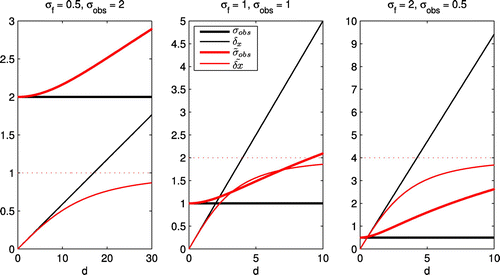
Fig. 1 shows the solution (12) for modified observation error variance and the corresponding increment vs. innovation for three combinations of observation error variance and state error variance in the case .

Figure 1. Behaviour of the solution (12) for (thick red line) and the associated increment (thin red line) vs. innovation d; calculated for three combinations of observation error variance and state error variance in the case . The black lines show non-modified variables and , and the dotted red lines indicate the maximal achievable increment of .

Expression (12) is indeed not the only possible solution that satisfies requirements (6(6) –8(8) ); however it is simple, smooth, and has only one tunable parameter. We will refer to it as ‘K-factor QC’.

3. Experiments

In this section, we demonstrate the effect of the proposed QC procedure on the performance of the system for both idealised and operational systems.

3.1. Experiments with a small model

The experiments with the small model below aim to test the KF-QC procedure in three situations: in nearly optimal settings; with observation outliers; and with model error. The 40-dimensional model by Lorenz and Emanuel (1998) is used. The model is based on the 40 coupled ordinary differential equations in a periodic domain:

Following Lorenz and Emanuel (1998), this system is integrated with the fourth-order Runge–Kutta scheme, using a fixed time step of 0.05, which is considered to be one model step.

The DA system uses the ensemble square root filter (ESRF Tippett et al., 2003) method with ensemble size of 35.

3.1.1. Experiment 1: a nearly optimal system

In this experiment, each element of the ‘true’ model state is observed at every time step with normally distributed error with standard deviation equal 1 (), and these observations are assimilated at every time step. Multiplicative inflation of 1% is used for stability of the system.

These settings have been used in numerous studies, following whi02a. They are known to result in a weakly nonlinear DA regime with mean analysis root mean square error (RMSE) about 0.178–0.180. The resulting system represents a good test bed for the effect of the KF-QC in a nearly optimal situation when the QC is supposed to be redundant.

Each run in this experiment is spun up for 500 cycles from an initial ensemble of random states from a long model run and then run for cycles. A run in Experiments 1–3 is considered invalid (diverged) if the mean analysis RMSE for the last 100 cycles exceeds 3. Runs with the same initial seed are started from the same initial conditions and assimilate the same sets of observations.

Fig. 2 shows the mean analysis RMSE over cycles depending on the K-factor. It also shows the RMSE for the system using the standard BC (1(1) ), when an observation is discarded if the corresponding innovation magnitude exceeds . Note that due to the run length smaller than normally required for a system with this model (Sakov and Oke, 2008, Section 4b), there is a relatively large variability of the mean RMSE for the runs started from different initial conditions; at the same time there is a fairly good continuity of results obtained in the runs started from the same initial conditions. (The smaller run length is adopted in this and following experiments to achieve balance between quantifying the system performance and the probability of breakdown.)

Figure 2. Mean analysis RMSE of a nearly optimal system with KF-QC and BC for three different initial conditions (seeds).

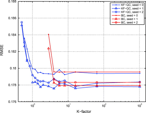
Figure 3. Performance of a system with non-Gaussian dense observations using KF-QC and BC for three different initial conditions (seeds).

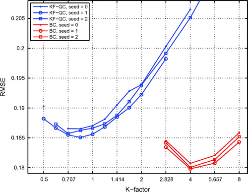
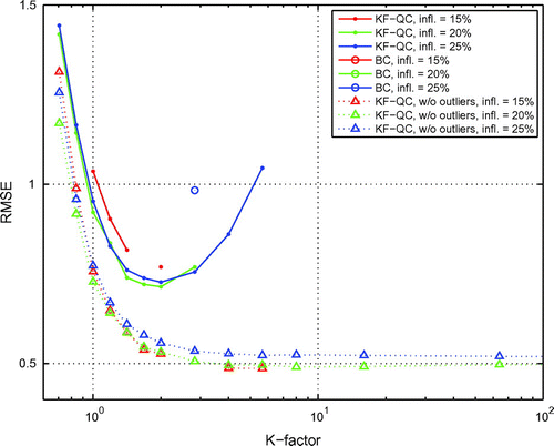
Figure 4. Performance of a system with non-Gaussian sparse observations using KF-QC.

The experiment shows that there is only a minor deterioration for the mean RMSE (of order of 1% or less) at , and the curves are essentially flat from approximately . The system using the standard BC shows basically no effect from it when convergence is achieved, from about , and significant loss of performance or divergence for smaller K. Note that on average only about 0.0026 observations per cycle are discarded by BC at , 0.19 at and 3.6 at . Indeed, in this experiment the observations with large innovations (more likely to be refused by BC) represent the most valuable observations in terms of moving the model state towards the true state.

3.1.2. Experiment 2: a system with non-Gaussian dense observations

This experiment is almost identical to Experiment 1, except that the observations are contaminated with rare outliers. Namely, with probability 0.995 the observation error is sampled from N(0, 1), and with probability of 0.005 it is sampled from N(0, 10). The DA system assumes that the error is distributed as N(0, 1).

Table 1. MAD of the forecast innovations for runs with different K-factors, averaged over all cycles.

	SLA (cm)	SST (K)	T (K)	S (PSU)
	0.0529	0.383	0.536	0.105
	0.0530	0.385	0.520	0.105
	0.0546	0.392	0.509	0.105

Table 2. Mean dissipated TKE over 3-day cycle, calculated as mean increment minus trend.

	J	0.94%
	J	1.30%
	J	2.01%

Both in Experiments 1 and 2, the system is in a regime when the observation error standard deviation (equal to or about 1) is much greater than the mean forecast error (about 0.2). This means that the analysis error is mainly defined by the previously assimilated observations rather than by those from the current cycle. Therefore, the experiment is characterised by abundant dense observations and rare outliers, when discarding an outlier should hardly affect the performance. This is perhaps an ideal case for application of BC. In contrast, KF-QC is a universal method that limits the impact of an outlier, but does not filter it out; hence it is not supposed to outperform BC in this case. The purpose of this experiment is to examine whether KF-QC is still able to manifest reasonable performance and robustness.

Figure 5. Total kinetic energy for a realistic DA system with different K-factor values.

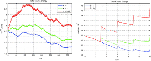
Fig. 3 shows the mean analysis RMSE of the systems with KF-QC and BC. As expected, BC performs robustly and is able to achieve the best overall performance, with the RMSE about 0.18 or slightly above. KF-QC yields a slightly worse performance, with the best mean RMSE of 0.185–0.187, and also shows good robustness by achieving convergence for a wide range of the K-factor.

3.1.3. Experiment 3: a system with non-Gaussian sparse observations

This experiment aims at creating a situation with much reduced redundancy in observations compared to Experiment 2, so that discarding observations or reducing their impact excessively can lead to the filter divergence. Specifically, all even elements of the model state are observed every 5 time steps. As in Experiment 2, the observations are contaminated with occasional outliers: with probability 0.96 the observation error is sampled from N(0, 0.4), and with probability of 0.04 it is sampled from N(0, 4). The DA system assumes that the error is distributed as N(0, 0.4). Each run is integrated for model steps, or DA cycles after a spin-up period of 200 cycles.

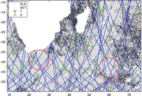
Figure 6. Observations assimilated in analyses in Fig. 11, on 1 July 2011. The red circles correspond to the regions shown in Fig. 11.

With these settings, in the absence of outliers the EnKF has little problem constraining the model, although it needs sufficient inflation to achieve long-term stability (about 1.20 or more). Due to the substantial nonlinearity in the system, there are occasional spikes in the forecast error exceeding the estimated forecast error by a factor of 4 or more (not shown).

In the presence of outliers, the QC has to reduce the impact (KF-QC) of or discard (BC) observations with large innovation magnitudes. Some of these observations are perfectly valid and represent spikes in innovation caused by the system’s nonlinearity. These observations are quite valuable for constraining the system, and discarding them can lead to the filter divergence. Therefore, the system needs to find balance between the need to discard or reduce the impact of outliers and the need to keep or not reduce excessively the impact of valid observations with large innovations.

Fig. 4 shows the mean analysis RMSE of the systems with KF-QC and BC for three different settings of inflation: 1.15, 1.20 and 1.25. It also shows the RMSE of the system with KF-QC assimilating observations without outliers.

Figure 7. SLA observations in Fig. 6.

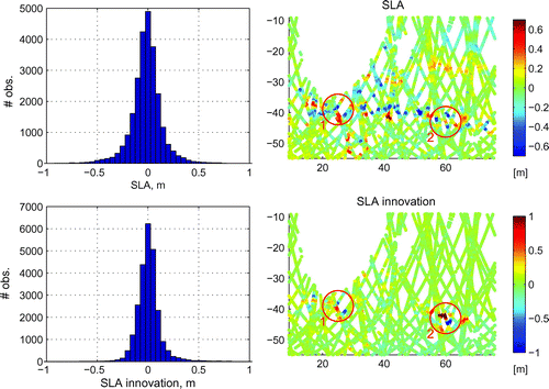
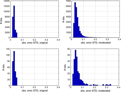
Figure 8. Observation error for SLA observations in Fig. 6 before and after applying the KF-QC with , for all SLA observations (upper row) and for observations with innovation magnitude exceeding 0.5 m (lower row).

The system with KF-QC performs stably with inflation set to 1.20 and 1.25, while with inflation of 1.15 it is prone to occasional divergence. The best performance is achieved with . The corresponding average modified observation error standard deviation is about (while the actual observation error standard deviation is ). The system with BC is only able to complete one run at a substantially worse performance.

3.2. Experiment with a realistic model

This section investigates using KF-QC in a realistic ocean DA system by conducting three runs with different values of the K-factor: 1, 2 and 999. The case is practically equivalent to running the system without KF-QC. All three runs start from the same initial condition obtained from a spun up system with and are run for the period from 1 July 2011 to 4 July 2012.

The DA system is based on a version of OFAM3 model (Oke et al., 2013). The model represents a version of MOM 4p1 set in domain from 75 S to 75 N. The grid has 0.1 horizontal resolution and 51 vertical layers. The model uses ERA-interim bulk forcing, a fourth-order Sweby advection method, General Ocean Turbulence Model - vertical mixing scheme and a scale-dependent isotropic Smagorinksy horizontal mixing scheme.

The DA system uses the ensemble optimal interpolation (EnOI) method with a three-day centred cycle, and assimilates satellite altimetry sea level anomalies (SLA) from the RADS database, sea surface temperature (SST) observations from the NAVO database and in situ T and S observations by Argo floats. The system uses a 144-member ensemble with members calculated as the difference between the 3-day and monthly averages from a long free model run. The system does not use any specific initialisation procedure (that is, initialises to analysis).

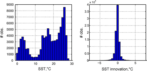
The histograms for SST observations are shown in Fig. 9.

Table 1 shows the mean absolute deviation (MAD) of the forecast innovations for these runs. KF-QC improves the system’s performance on SLA and SST but worsens on subsurface temperature (T). Therefore, in terms of the MAD of the forecast innovation there is no clear benefit from applying KF-QC to this system; however, other characteristics of these runs contain some significant differences.

Fig. 5 shows the three-hourly time series of the total kinetic energy (TKE) of the ocean for the whole time period (left panel) and for the four cycles (right panel) that include the last cycle of spin-up and the first three cycles of runs with different K-factors. At each cycle, there is a sharp increase in the TKE followed by a gradual decrease; there are also smaller inertial oscillations with the period 0.6–0.7 days.

While there are situations when ocean currents and fronts are expected to strengthen due to DA (e.g. when they cannot be sustained by the model because of an insufficient resolution), this strengthening rarely represents a desirable feature of the system. A higher level of the TKE in a data assimilating model is typically associated with larger analysis increments and instabilities.

From Fig. 5, the system with has the largest increments in the TKE from the forecast to analysis, followed by the systems with and . The mean increment of TKE is  J (2.05% of the TKE) for the system with ;  J (1.19%) for , and  J (0.74%) for . At the end of the run period, the system with has about 37% larger TKE than the system with , and 20% larger TKE than the system with . The average trend of the TKE is  J (0.04%) per cycle for ,  J (-0.11%) for , and  J (0.20%) for . Therefore, given that the experiments were run for 133 DA cycles, for all three systems the TKE increments are mainly not sustained by the model; however, the average dissipated TKE per cycle is by far greatest in the system with , both in absolute ( J) and relative (2.01%) terms, followed by the systems with ( J, 1.30%) and ( J, 0.94%) (Table 2). This indicates that the system without KF-QC works in a more ‘stiff’ regime, with larger increments and imbalances. It comes to an equilibrium between injected and dissipated energy at a substantially higher energy level than the other two systems.

Figure 9. Histograms of SST observations in Fig. 6.

We will now analyse the effect of DA with different K-factors on the model fields. Specifically, we will look at the model velocity fields before and after the very first cycle where the analyses are calculated with different K-factors.

Figs. 6 depicts locations of all superobservations assimilated at this cycle (on 1 July 2011). The superobservations were obtained by collating all observations of one kind (SLA, SST, T, S) within each model grid cell. There are total 24946 SLA observations, 86460 SST observations, 2756 in situ T observations and 3010 in situ S observations.

Figure 10. Sea surface height and SST ensemble spread in the ocean DA system.

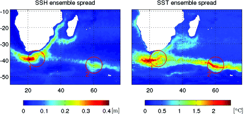
Figure 11. Surface velocity magnitude in a realistic ocean DA system: the forecast, and analyses obtained with different K-factors.

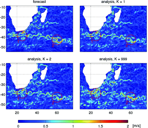
Fig. 7 shows histograms and maps for the SLA observations and corresponding innovations. There are two regions where the magnitude of innovation reaches or exceeds 1 m, one about (25 E, 40 S), and another about (60 E, 43  S). They mainly coincide with the regions 1 and 2 designated by the red circles. Such a large magnitude of innovation means that the model is mainly not constrained there. This creates conditions favourable for applying the KF-QC, when valid observations have large innovation due to the divergence of the model. These observations would be discarded by the BC or produce unbalanced analysis if assimilated without moderation; with KF-QC they still can have a positive impact on the system.

Fig. 8 shows histograms of the assumed SLA observation error standard deviation (STD) before and after application of the KF-QC with , both for all SLA observations (upper row) and for observations with innovation magnitude exceeding 0.5 m. They illustrate the effect of applying the KF-QC on the observation error standard deviation.

Fig. 10 shows the surface velocity field for the Agulhas region for the very first cycle where analyses are calculated with different K-factors. There are some significant differences in the surface velocity field in some regions in the analyses calculated with different K-factors. These differences are particularly well manifested in Regions 1 and 2 highlighted by red circles in Figs. 6–10. There is nothing special about the observations in these regions (Fig. 6), so the large increments in them must be mainly associated with more chaotic flow leading to larger innovations and/or ensemble spread (Fig. 11) than elsewhere.

The system with no KF-QC () has a rather discontinuous and visually chaotic analysed flow in Regions 1 and 2, with structure much different to that in the forecast. Such a dramatic change in the system state assumes a high degree of optimality in the DA system, including a nearly perfect model, linearity and the use of an advanced DA method. Neither of these pre-conditions are likely to be satisfied here or in most realistic DA systems; therefore, the behaviour seen with should, generally, be avoided. Moreover, even in a situation with a nearly perfect model and dense observations, the use of static ensemble in the EnOI results in increments not related to the flow of the day, so that large increments can lead to an unrealistic (and, likely, strongly unbalanced) analysis. In contrast, the systems with KF-QC generally preserve the flow structure from the forecast to analysis, both for and . This is a desired regime for a realistic DA system.

4. Discussion and conclusions

We proposed an adaptive QC procedure referred to as KF-QC. It is based on presumptions that (1) large increments in the analysis should be avoided and (2) simply discarding the associated observations can often prevent assimilating important information by the DA system. KF-QC smoothly increases the observation error so that the magnitude of the increment does not exceed a multiple (called the K-factor) of the estimated state error.

As demonstrated in Experiment 1, in nearly optimal cases for moderate or large values of the K-factor (say, ) the KF-QC does not affect the model performance. In this sense, KF-QC is non-intrusive and can be used by default in practical DA. It has been used for considerable time in the EnKF-based operational ocean DA system TOPAZ (Sakov et al., 2012, Section 3.2) , and since early 2016 in the EnOI-based operational ocean DA system OceanMAPS v3 run by the Australian Bureau of Meteorology (Sakov, 2014, Section 2.7.3).

In situations with observation outliers, the KF-QC achieves better robustness of the system compared to BC, at a cost of a rather minor deterioration in performance (Exp. 2). It achieves both good robustness and performance in situations with simultaneous presence of observation outliers and significant nonlinearity (Exp. 3). From our experience with operational ocean forecasting, due to improved quality control by observational data providers, outliers have became less frequent in recent years. Therefore, handling of observation outliers becomes relatively less important compared to handling of instances of large innovations caused by other reasons, such as initial conditions, model error or nonlinearity.

When tested with a realistic global eddy resolving ocean DA system over a period of 1 year, the KF-QC has not yielded obvious benefits in terms of the innovation error, but produced an arguably more balanced output, with overall smaller increments, including much smaller increments in the total kinetic energy of the ocean. This is a desirable feature for reanalysis products used for providing open boundary conditions for limited area models. When first used in OceanMAPS, the KF-QC made it possible to assimilate subsurface T and S observations in regions with large discrepancies in the initial model state. Previously such observations were routinely discarded by BC, resulting in long-term systematic errors.

Apart from the good performance and universality, the systems with the KF-QC have also shown good stability manifested in smooth dependence on the K-factor around the optimal value. By contrast, in Experiment 1 the system with BC exhibits a break-down behaviour for , and in Experiment 3 it could only achieve convergence once in three series of runs with different inflation factors.

The aims and ideas behind the KF-QC are very similar to those manifested for the Huber norm QC (Tavolato and Isaksen, 2015). ‘... the relaxation of the background QC ... is a very important side benefit of the Huber norm method, because it makes observations with large departures active, so the data get a chance to influence the analysis’. The two procedures can perhaps behave similarly when applied to individual observations (e.g. by using their Equation 4), although the KF-QC with its single tunable parameter can be easier to use, particularly in ensemble-based systems.

Because the KF-QC targets not only the observation outliers, but rather a variety of potential issues that may lead to large increments, it perhaps has functionality outside observation QC in a narrow sense. We still qualify it as a QC procedure because, firstly, it can be seen as a simple modification of the common BC, and secondly, the other procedures with similar functionality, such as the VarQC, are also considered to be QC procedures.

The proposed procedure is rather simple, even simplistic, as it only considers the increment in observation space for a single observation. Limiting increment for individual observations does not guarantee that the overall increment will remain small. It would be nice to develop a consistent method limiting the total magnitude of the increment depending on the estimated state error to limit the potential imbalance of the analysis, but that, much more challenging, problem is outside the scope of this paper and perhaps outside the scope of observation QC.

Because of its serial character, the KF-QC works best in situations with sparse observations. In the context of ocean DA, this means that it will be more effective in limiting the increment from subsurface S and T and track SLA observations, and less effective for that from SST observations because of a typically large number of local observations assimilated at a given location. Note that even in the case of dense observations the KF-QC still effectively reduces the impact from potential observation outliers.

Acknowledgements

The authors would like to thank two anonymous reviewers for their helpful suggestions.

Notes

No potential conflict of interest was reported by the authors.

References

- Anderson, E. and Järvinen, H. 1999. Variational quality control. Q. J. R. Meteorol. Soc. 125, 697–722.
- Dee, D. P., Rukhovets, L., Todling, R., da Silva, A. M. and Larson, J. W. 2001. An adaptive buddy check for observational quality control. Q. J. R. Meteorol. Soc. 127, 2451–2471.
- Dee, D. P., Uppala, S. M., Simmons, A. J., Berrisford, P., Poli, P., and co-author. 2011. The ERA-Interim reanalysis: Configuration and performance of the data assimilation system. Q. J. R. Meteorol. Soc. 137, 553–597.
- Dharssi, I., Lorenc, A. C. and Ingleby, N. B. 1992. Treatment of gross errors using maximum probability theory. Q. J. R. Meteorol. Soc. 118, 1017–1036.
- Huber, P. J. 1964. Robust estimation of a location parameter. Ann. Math. Stat. 35, 73–101.
- Huber, P. J. and Ronchetti, E. M. 2009. Generalities -- Robust Statistics Hoboken, NJ: John Wiley & Sons, pp. 1–21.
- Ingleby, N. B. and Lorenc, A. C. 1993. Bayesian quality control using multivariate normal distributions. Q. J. R. Meteorol. Soc. 119, 1195–1225.
- Lorenc, A. C. 1981. A global three-dimensional multivariate statistical interpolation scheme. Mon. Wea. Rev. 109, 701–721.
- Lorenc, A. C. 2002. Atmospheric Data Assimilation and Quality Control Springer, Berlin Heidelberg, Berlin, Heidelberg, pp. 73–96.
- Lorenz, E. N. and Emanuel, K. A. 1998. Optimal sites for suplementary weather observations: Simulation with a small model. J. Atmos. Sci.
- Oke, P. R., Griffin, D. A., Schiller, A., Matear, R. J., Fiedler, R., and co-authors. 2013. Evaluation of a near-global eddy-resolving ocean model. Geosci. Model Dev. 6, 591–615.
- Sakov, P. 2014. EnKF-C user guide. J. Appl. arXiv:1410.1233 [cs.CE].
- Sakov, P., Counillon, F., Bertino, L., Lisæter, K. A., Oke, P. R. and co-authors. 2012. TOPAZ4: an ocean-sea ice data assimilation system for the North Atlantic and Arctic. Ocean Sci. 8, 633–656.
- Sakov, P. and Oke, P. R. 2008. Implications of the form of the ensemble transformations in the ensemble square root filters. Mon. Wea. Rev. 136, 1042–1053.
- Tavolato, C. and Isaksen, L. 2015. On the use of a Huber norm for observation quality control in the ECMWF 4D-Var. Q. J. R. Meteorol. Soc. 141, 1514–1527.
- Tippett, M. K., Anderson, J. L., Bishop, C. H., Hamill, T. M. and Whitaker, J. S. 2003. Ensemble square root filters. Mon. Wea. Rev. 131, 1485–1490.
- Whitaker, J. S. and Hamill, T. M. 2002. Ensemble data assimilation without perturbed observations. Mon. Wea. Rev. 130, 1913–1924.