Continued warming, salinification and oxygenation of the Greenland Sea gyre

Abstract

The Greenland Sea gyre is one of the few areas where the water column is ventilated through open ocean convection. This process brings both anthropogenic carbon and oxygen from the atmosphere and surface ocean into the deep ocean, and also makes the Greenland Sea gyre interesting in a global perspective. In this study, a combination of ship- and float-based observations during the period 1986–2016 are analysed. Previous studies have shown warming and salinification of the upper 2000 m until 2011. The extended data record used here shows that this is continuing until 2016. In addition, oxygen concentrations are increasing over the entire period. The changes in temperature, salinity, and especially oxygen have been more pronounced since the turn of the century. This period has also been characterised by deeper wintertime mixed-layer depths, linking the warming, salinification and oxygenation to strengthened ventilation in the Greenland Sea gyre after 2000. The results also demonstrate that the strengthened ventilation can be tied to advection of warmer and more saline surface water from the North Atlantic through the Faroe-Shetland Channel. This advection has led to more saline surface waters in the Greenland Sea gyre, which is contributing to the deeper wintertime mixed layers.

Keywords:

• Greenland Sea
• ventilation
• hydrographic changes
• observations
• convection

1. Introduction

The Greenland Sea is globally important as one of the few locations where open ocean convection, a process which brings anthropogenic CO₂ and oxygen from the surface to the deep ocean (e.g. Fröb et al., 2016), occurs. The Greenland Sea is important for anthropogenic carbon storage (e.g. Olsen et al., 2010), and for global ocean ventilation through its likely contribution to the lower limb of the Atlantic Meridional Overturning Circulation (AMOC; e.g. Eldevik et al., 2009; Våge et al., 2015). It is not known how much the Greenland Sea currently contributes to AMOC, and over time estimates have ranged from the Greenland Sea being a major source (e.g. Swift et al., 1980; Strass et al., 1993), via contributing almost nothing (Mauritzen, 1996), to being a non-negligible source (e.g. Olsson et al., 2005; Jeansson et al., 2008). Today, the general consensus is that regardless of the magnitude of the contribution from the Greenland Sea to AMOC, it is mainly derived from the intermediate water masses and not the deep water masses (e.g. Eldevik et al., 2009). This changing view on the importance of the Greenland Sea for AMOC has evolved in conjunction with observations of extensive changes in its water mass properties as documented by e.g. Blindheim and Rey (2004), Karstensen et al. (2005), Ronski and Budéus (2005), Latarius and Quadfasel (2010, 2016), Rudels et al. (2012) and Somavilla et al. (2013). Perhaps most importantly, due to the cessation of the deep-water (>2000 m) renewal since the 1980s (Schlosser et al., 1991), only the intermediate layers have been ventilated and both temperature and salinity in the upper 2000 m of the water column have increased more than in the deep ocean (e.g. Karstensen et al., 2005; Latarius and Quadfasel, 2010, 2016). Furevik et al. (2002) showed that the salinity increase is a reversal of a long-term trend of decreasing salinity in the Nordic Seas that had been going on since the 1960s. These long-term changes are also evident in the decadal climatologies of Korablev et al. (2014).

Previous work has either focused on the 1990s and early 2000s or the period after 2001, largely because of the difference in major data sources in these periods. For the period before 2001, data are only available from relatively few (1–2 per year) hydrographic cruises while beginning in 2001 the deployment of Argo floats in the Greenland Sea has led to a large increase in the amount of available hydrographic data for all seasons. Here, we bridge the gap between analyses utilising only ship-based data (e.g. Furevik et al., 2002; Karstensen et al., 2005) and analyses focusing on the Argo-era (e.g. Latarius and Quadfasel, 2010, 2016) by utilising available data in the period 1985 to 2016, from both ship-based hydrographic surveys and Argo floats. Compared to Latarius and Quadfasel (2016), which ends in 2011, we also extend the period studied by five years. This relatively long-time series of observations enables us to capture the longer term perspective of hydrographic changes in the Greenland Sea gyre leading to improved understanding of the origin of these changes.

2. Data and methods

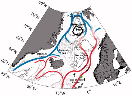
The area of interest is shown in Fig. 1, and the Greenland Sea gyre was defined according to Moore et al. (2015), using the surface dynamic height relative to 500 m depth. The main data used here are the temperature, salinity and oxygen profiles taken during the years 1985–2016 in the International Council for the Exploration of the Sea (ICES) database, and the temperature and salinity profiles taken during the years 2001–2016 were obtained by Argo floats in the Greenland Sea. The Argo data were collected and made available by the Coriolis project and programmes that contribute to it (http://www.coriolis.eu.org, http://doi.org/10.17882/42182). Only delayed mode quality controlled profiles were included in this analysis. In addition, temperature, salinity and oxygen profiles were extracted from GLODAPv2 (Key et al., 2016; Olsen et al., 2016), and from three recent hydrographic cruises (with R/V Johan Hjort in 2015 and with R/V G. O. Sars in 2013 and 2016) covering the Greenland Sea. On the R/V Johan Hjort cruise and the R/V G. O. Sars cruise in 2016 oxygen was analysed on-board by Winkler titration of samples drawn from Niskin bottles, to an uncertainty of not more than 1%. GLODAPv2 oxygen data have been extensively quality controlled and are accurate to within 1% (Olsen et al., 2016). On the R/V G. O. Sars cruise in 2013, oxygen was measured by a SBE43 oxygen sensor, calibrated six months prior to the cruise, attached to the CTD profiler. These data were quality controlled using cross-over analysis (Lauvset and Tanhua, 2015) against the historical data and have an uncertainty of not more than 1%. In addition to the water column data from the Greenland Sea, we used the temperature and salinity time-series data of Atlantic Water in the Faroe-Shetland Channel (green X in Fig. 1) regularly published in the ICES report on ocean climate (Hughes et al., 2011).

Fig. 1. Map of the Nordic Seas. The grey lines show (from light to dark) the 500, 1000, 1500, 2000, 3000 and 4000 m isobaths. The bold black contour outlines our definition of the Greenland Sea gyre, and the green x marks the position of the Faroe-Shetland Channel hydrographic time series. The generalised circulation pattern in the region is shown with red and blue arrows indicating warm and cold currents, respectively.

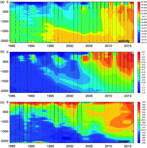
For the temperature and salinity analyses presented, only wintertime (February–April) observations were used. For the estimation of temporal trends, the observations were first interpolated to the given depth (500, 1000 or 1500 m) using a piecewise cubic Hermite spline function and then averaged over each winter. The interpolation distances (from the observed depth) are less than 3 m. Using annual averages minimises the potential bias introduced by the much more frequent observations in the Argo period. For oxygen, there are very few wintertime profiles, so all available profiles from all seasons have been used. To calculate the oxygen inventory, the individual profiles were first vertically interpolated onto a fixed depth profile (0, 10, 20, 30, 40, 50, 100, 150, 200, 250, 300, 350, 400, 450, 500, 600, 700, 800, 900, 1000, 1250, 1500, 1750 and 2000 m) using a piecewise cubic Hermite function (and maximum distance criteria as described by Key et al., 2016). For visualisation (Fig. 2), the winter mean profiles were also interpolated onto a regular grid in the time-depth plane, but the spatially interpolated data were not used for analysis.

Fig. 2. Interpolated time series of (a) salinity, (b) potential temperature (θ, °C), (c) oxygen (μmol kg⁻¹) in the Greenland Sea gyre. The black dots indicate the wintertime (February–April) average profiles for salinity and θ, and the annual average profile for oxygen.

The wintertime mixed-layer depth in the Greenland Sea gyre was determined for each profile following the procedure used by Våge et al. (2015) for the Iceland Sea. The procedure combines two automated (Lorbacher et al., 2006; Nilsen and Falck, 2006) and one manual routine (Pickart et al., 2002). The manual routine was used only when the first two routines failed to accurately determine the mixed-layer depth, typically because of small density differences between the mixed layer and the deeper part of the water column, or due to mixed layers isolated from the surface (Brakstad et al., in review).

3. Observed changes in Greenland Sea hydrography

Observations from the Greenland Sea gyre in 1986–2016 (all seasons) show increased oxygen concentrations in the top 2000 m since the late 1990s (Fig. 2a). This increase is a clear evidence of convection ventilating the intermediate depth ocean in this region. Concurrent wintertime observations show that in the same period there has been an overall increase in both temperature and salinity throughout the upper water column (0–2000 m, Fig. 2b and 2c). Latarius and Quadfasel (2016) showed this warming and salinification until 2011, and at 1000 m the trend continues from 2011 to 2016 at the same rate (0.020 ± 0.002 for temperature and 0.0008 ± 0.0001 for salinity). There are, however, large inter-annual variations and shorter periods of decrease in both variables in the time period studied here. Different depth layers also show different trends and different inter-annual variations, so here we focus on the observed changes at intermediate depths (500–1500 m, Fig. 3, Table 1). At 500 m depth, the temperature and salinity were both variable and did not exhibit any significant trend until the turn of the century. After 2003, the temperature increased relatively steadily to –0.22 °C in 2016 (compared to –1.11 in 1986). Salinity increased by 0.026 ± 0.001 in the same period. At 1000 m depth, the temperature increased from 1986 until 1995, but then decreased by 0.14 ± 0.02 °C until a new warming period began around the year 2000. By 2016, temperatures had risen by 0.63 ± 0.07 °C from –1.18 °C in 1986. Salinity at 1000 m depth exhibited inter-annual variability, but remained relatively unchanged until 2001 when it began increasing, from 34.880 to 34.916 by the year 2016. The overall temperature increase at 1500 m is slightly smaller than that at 1000 m (0.50 ± 0.02 °C), but at this level, the salinity increased strongly in the 1990s (from 34.887 in 1991 to 34.906 in 1998) followed by a brief decrease. After 2005, the changes in salinity at 1000 and 1500 m depth have been similar.

Fig. 3. Figure showing the temporal evolution of winter mean (circles) salinity and potential temperature (θ, °C) for three different depths in the Greenland Sea gyre. The shaded area indicates one standard deviation of the mean of all data in each year.

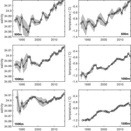
Table 1. Trends in winter (February–April) temperature and salinity for three different depth levels over the years 1985 to 2016. To limit the effect of sampling bias, the regression is based on the mean of winter observations each year. The uncertainty is estimated using a Monte Carlo simulation (1000 runs) of possible slopes within the one standard deviation confidence interval of each year (as shown in Fig. 3). Note that all regressions are statistically significant with a p-value of zero for a Student’s t-test.

	Temperature			Salinity
	slope ± uncertainty	r^2	RMSE	slope ± uncertainty	r^2	RMSE
500 m	0.025 ± 0.005	0.81	0.11	0.002 ± 0.0003	0.72	0.01
1000 m	0.020 ± 0.003	0.90	0.07	0.001 ± 0.0003	0.66	0.006
1500 m	0.020 ± 0.001	0.93	0.05	0.0004 ± 0.0005	0.27	0.006

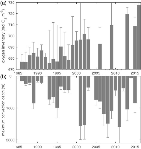
The water making up the intermediate depth layer in the Greenland Sea is a result of cooling of the warm, saline Atlantic Water and subsequent mixing with the colder, fresher Polar Water found to the west of the gyre (e.g. Eldevik and Nilsen, 2013). The evolution of the temperature and salinity properties of the intermediate depth Greenland Sea gyre from 1986 to 2016 is summarised in Fig. 4a, and the increasing influence of the warm and saline Atlantic Water – which at this latitude has an average temperature of 4.0 ± 0.7 °C and salinity of 35.08 ± 0.05 – is evident. The concurrent increase in oxygen concentrations in this period is shown in Fig. 4b, which also visualises how the oxygen would have changed if driven by the gas solubility alone. Since the oxygen changes are clearly not driven by solubility changes, they must represent ventilation by convection, the consequence of which is a warmer, more saline, and more oxygenated gyre. The oxygen inventory (Fig. 5a) in the top 2000 m of the Greenland Sea gyre increased by 50.0 ± 19.8 mol m⁻² between 1986 and 2016, but 65% of that increase happened between 2000 and 2016 suggesting that the ventilation strengthened around the turn of the century.

Fig. 4. Diagram of wintertime (February–April): (a) potential temperature and salinity; (b) potential temperature and oxygen. All points are annual averages over 500–1500 m in the Greenland Sea gyre in period 1985–2016. The arrow in (b) indicates the direction of change if only the solubility of oxygen changed.

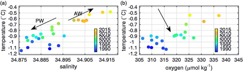
Fig. 5. Time series of (a) oxygen inventory (mol m⁻²) integrated over the top 2000 m of the Greenland Sea gyre; (b) maximum wintertime mixed-layer depths (m) in the Greenland Sea gyre. For both (a) and (b) the error bars indicate one standard deviation of the annual average.

4. Mechanisms behind, and impacts of, the observed changes in the Greenland Sea

The frequency of deep mixing has increased after 2000. According to our observations, seven winters (2001, 2002, 2007, 2008, 2009, 2011 and 2013) have had mixed-layers deeper than 1000 m after 2000, while the deepest recorded mixed layer between 1986 and 1999 was 938 m (Fig. 5b). The evolution of wintertime mixed layers in the Greenland Sea during the 1986–2016 period is thus best described as two distinct periods: one dominated by relatively shallow (<1000 m) mixed layers lasting until the late 1990s; and another, beginning around 2000, dominated by relatively deep (>1000 m) mixed layers. This is consistent with the convection depths found by Ronski and Budéus (2005), which are shallower in the 1990s than in the new millennium. Ronski and Budéus (2005) used a much shorter time series than this study, but the consistency between the studies still confirm that the deeper mixed layers observed after 2000 are not entirely due to the more frequent observations in the Argo era. The coinciding timing of the strengthened ventilation and the deepening mixed layers in the Greenland Sea gyre is also another indication that the oxygen increase is due to convection, which is confirmed by a significant correlation between mixed-layer depth and oxygen inventory (Fig. 4a, r = 0.51, p-value = 0.025).

The observed interior ocean changes do not explain why the Greenland Sea in the late 1990s transitioned from having predominantly shallow wintertime mixed layers to having predominantly deep wintertime mixed layers; the wintertime heat loss exceeded 200 Wm² several years in the 1990s too (Brakstad et al., in review). In addition, Moore et al. (2015) showed that a reduction in wintertime sea ice cover and the atmosphere warming faster than the ocean in the Nordic Seas has resulted in a significant reduction of the turbulent air-sea heat fluxes over the Greenland Sea gyre since the mid-1990s. They demonstrate that reduced atmospheric forcing reduces the wintertime mixed layer depth in the Greenland Sea, but the observations used in this study show that the opposite has happened, the wintertime mixed-layers have deepened. Clearly, there are more factors than the wintertime heat loss that influence the convective activity in the Greenland Sea gyre, but it should be noted that all years with mixed-layers deeper than 1000 m had a wintertime surface heat loss exceeding 200 Wm⁻² (Brakstad et al., in review). This is consistent with the one-dimensional model used by Moore et al. (2015), which indicate that once the heat loss exceeds 150 Wm⁻² the convection becomes much deeper and more sensitive to small changes in atmospheric forcing. This is primarily because 150 Wm⁻² is sufficiently strong heat loss to erode the shallow ocean stratification. While idealised, their model adequately reproduces observations in two selected years (2008 and 2012) and they make a strong case for the conclusion that reduced atmospheric forcing, if it continues, would lead to the Greenland Sea gyre experiencing primarily shallow convection in the future as winters with sufficiently strong heat loss become more rare.

An additional component is provided by Latarius and Quadfasel (2016). They used Argo data up to 2011 to show that high summertime surface salinities in the Greenland Sea tend to lead to deep mixed layers the following winter, possibly because it leads to weaker shallow ocean stratification. Wintertime heat loss is still the dominant factor for convection, so this tendency does not mean that surface salinities alone are determining the depth of wintertime mixed layers in the Greenland Sea gyre. However, a significant correlation (r = 0.52, p-value = 0.013) between surface salinity and mixed-layer depth the following winter for the 1986–2016 period suggest that high summertime salinities are favourable for deep wintertime mixing. So does the fact that, with the exception of 2001, for all years where the wintertime mixed-layer exceeds 1000 m the surface salinity anomalies the previous summer is at least 0.1 above the 1985–2016 surface salinity mean (not shown, see also Brakstad et al., in review). Moore et al. (2015) highlights that the gyre needs to be weakly stratified at mid-depth in order for convection to happen, and it would appear that the surface salinities are an additional important part of the environmental conditioning necessary for convection.

Since the mid-1990s, the temperature and salinity of the Atlantic Water entering the Nordic Seas from the North Atlantic have increased (Fig. 6). Surface ocean salinity anomalies in the Nordic Seas originate mostly from further south, in the Atlantic Ocean (Glessmer et al., 2014), and have been linked to the intensity and shape of the North Atlantic Subpolar gyre (Häkkinen and Rhines, 2004; Hátún et al., 2005). As a result of the observed changes in the Atlantic Water inflow, the temperature and salinity in the Atlantic Water of the Norwegian Sea became relatively high during the 2000s (Skagseth and Mork, 2012; Mork et al., 2014), reversing the long-term decrease in salinity observed until the mid-1990s (Furevik et al., 2002; Korablev et al., 2014).

Fig. 6. Time series of (a) potential temperature anomalies and (b) salinity anomalies in the core of Atlantic Water in the Faroe-Shetland Channel (black bars), and the surface waters (<150 m) of the Greenland Sea gyre (red line).

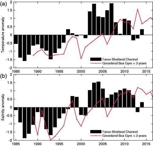
Previous studies (e.g. Latarius and Quadfasel, 2016) have also found that the warming in the Atlantic layer of the Greenland Sea until 2011 was comparable to that in the Fram Strait, and Latarius and Quadfasel (2016) suggest that part of the warming in the Greenland Sea is caused by exchange with the Norwegian Atlantic Current. However, studies using surface drifters (Koszalka et al., 2011, 2013) and Argo floats (Voet et al., 2010) show that there is a very limited exchange between the Norwegian Atlantic Current and the Greenland Sea gyre. Rather, most exchange occurs when the northward flowing Atlantic Water reaches the Fram Strait and a westward branch enters the southward East Greenland Current becoming the Return Atlantic Water (RAW). RAW is then entrained into the Greenland Sea gyre on the way to the south as confirmed in several previous studies (e.g. Mauritzen, 1996; Rudels et al., 1999; Håvik et al., 2017). This is corroborated by our analyses which show a strong cross-correlation between anomalies in the core of Atlantic Water in the Faroe-Shetland Channel and surface anomalies (<150 m) in the Greenland Sea gyre. These cross-correlations are 0.80 and 0.72 for salinity and temperature, respectively (both with a three-year lag and normalised such that the autocorrelation at zero lag equals one, Fig. 6). This result is consistent with the northward propagation of surface ocean hydrographic anomalies as presented by Holliday et al. (2008) that indicated 3–4 years lag-time between 57°N and the Fram Strait (78°N). Thus, the warm and saline Atlantic Water entering the Nordic Seas through the Faroe-Shetland Channel likely exert influence on the water column in the entire upper 2000 m of the Greenland Sea gyre.

As mentioned earlier, intermediate water masses from the Greenland Sea contribute to AMOC (e.g. Olsson et al., 2005; Jeansson et al., 2008; Eldevik et al., 2009), and it is clear that part of the necessary transformation takes place in the Greenland Sea (e.g. Latarius and Quadfasel, 2016). It is outside the scope of this paper to quantify how the changes in water mass characteristics observed in the Greenland Sea would affect AMOC, but any potential impact is likely to be small if not negligible. Latarius and Quadfasel (2016) find that increased freshwater content in the Greenland Sea would not affect the northern limb of AMOC so the reverse (increased salinity) is also likely true. In addition, recent work shows that the density of Greenland Sea Arctic Intermediate Water has not changed (Jeansson et al., 2017) and that the volume transport of overflow water has remained relatively constant (Hansen et al., 2015) in the time period of interest.

5. Summary and conclusions

In this study, we have described how temperature, salinity and oxygen increased at intermediate depth in the Greenland Sea gyre in the period from 1986 to 2016. The oxygen changes provide clear evidence of ventilation through a convection process. We also show how the wintertime mixed-layer depth has more frequently been deeper than 1000 m after the year 2000, and the extended time series used here supports a previously published (Latarius and Quadfasel, 2016) tendency of high-surface salinity leading to deep mixed-layers the following winter. This suggests that even though wintertime heat loss is the driving force behind deep convection, the increasing surface salinity in the Greenland Sea gyre has created more favourable conditions for convection. The increasing surface salinity comes from the Atlantic Water entering the Nordic Seas through the Faroe-Shetland Channel, as shown by the strong correlation between this and the surface changes (of both temperature and salinity) in the gyre. Over the 1985–2016 period, this has caused warming, salinification and oxygenation in the upper 2000 m of the Greenland Sea gyre. Perhaps most importantly, the Greenland Sea gyre is, like the Irminger Sea (Fröb et al., 2016), becoming more oxygenated in a time period where much of the oceans elsewhere are suffering deoxygenation (e.g. Schmidtko et al., 2017).

Acknowledgements

The ICES data were downloaded from http://ices.dk/marine-data/data-portals/Pages/ocean.aspx; the Argo data downloaded from http://www.argodatamgt.org/Access-to-data/Argo-data-selection. The Argo data were collected and made freely available by the International Argo Program and the national programmes that contribute to it (http://www.argo.ucsd.edu, http://argo.jcommops.org). The Argo Program is part of the Global Ocean Observing System. The Faroe-Shetland Channel time-series data are available at http://ocean.ices.dk/iroc/.

Disclosure statement

No potential conflict of interest was reported by the authors.

Additional information

Funding

This work has been funded the Center for Climate Dynamics of the Bjerknes Centre through a Fast-Track initiative grant, and from the Research Council Norway through the project VENTILATE (229791). Additional support was provided from the Research Council Norway under Grant agreement no. 231647 (K. Våge) and the Bergen Research Foundation under grant BFS2016REK01 (A. Brakstad and K. Våge). This is a contribution to the strategic project BIGCHANGE of the Bjerknes Centre for Climate Research. The authors thank Kristin Jackson and the crew of R/V Johan Hjort for collecting and analysing oxygen and salinity samples, and Lisbeth Håvik for valuable discussions regarding the water masses of the Greenland Sea.

References

- Blindheim, J. and Rey, F. 2004. Water-mass formation and distribution in the Nordic Seas during the 1990s. ICES J. Marine Sci. 61, 846–863. DOI:10.1016/j.icesjms.2004.05.003.
- Brakstad, A., Våge, K., Håvik, L. and Moore, G. W. K. In review. Water mass transformation in the Greenland Sea during the period 1986–2016. J. Phys. Oceanogr.
- Eldevik, T. and Nilsen, J. E. O. 2013. The Arctic-Atlantic thermohaline circulation. J. Clim. 26, 8698–8705. DOI:10.1175/jcli-d-13-00305.1.
- Eldevik, T., Nilsen, J. E. O., Iovino, D., Olsson, K. A., Sandø, A. B. and co-authors. 2009. Observed sources and variability of Nordic seas overflow. Nature Geosci. 2, 406–409. DOI:10.1038/ngeo518.
- Fröb, F., Olsen, A., Våge, K., Moore, G. W. K., Yashayaev, I. and co-authors. 2016. Irminger Sea deep convection injects oxygen and anthropogenic carbon to the ocean interior. Nat. Comms. 7, 13244. DOI:10.1038/ncomms13244.
- Furevik, T., Bentsen, M., Drange, H., Johannessen, J. A. and Korablev, A. 2002. Temporal and spatial variability of the sea surface salinity in the Nordic Seas. J. Geophys. Res. 107, 16. DOI:10.1029/2001jc001118.
- Glessmer, M. S., Eldevik, T., Våge, K., Nilsen, J. E. Ø. and Behrens, E. 2014. Atlantic origin of observed and modelled freshwater anomalies in the Nordic Seas. Nature Geosci. 7, 801–805. DOI:10.1038/ngeo2259.
- Hansen, B., Larsen, K. M. H., Hatun, H., Kristiansen, R., Mortensen, E. and co-authors. 2015. Transport of heat, and salt towards the Arctic in the Faroe Current 1993-2013. Ocean Sci. 11, 743–757. DOI:10.5194/os-11-743-2015.
- Hátún, H., Sandø, A. B., Drange, H., Hansen, B. and Valdimarsson, H. 2005. Influence of the Atlantic subpolar gyre on the thermohaline circulation. Science. 309, 1841–1844. DOI:10.1126/science.1114777.
- Häkkinen, S. and Rhines, P. B. 2004. Decline of subpolar North Atlantic circulation during the 1990s. Science. 304, 555–559. DOI:10.1029/2008jc004883.
- Håvik, L., Vage, K., Pickart, R. S., Harden, B., von Appen, W. J. and co-authors. 2017. Structure and variability of the Shelfbreak East Greenland current north of Denmark strait. J. Phys. Oceanogr. 47, 2631–2646. DOI:10.1175/jpo-d-17-0062.1.
- Holliday, N. P., Hughes, S. L., Bacon, S., Beszczynska-Moller, A., Hansen, B. and co-authors. 2008. Reversal of the 1960s to 1990s freshening trend in the northeast North Atlantic and Nordic Seas. Geophys. Res. Lett. 35, L03614. DOI:10.1029/2007gl032675.
- Hughes, S. L., Holliday, N. P. and Beszczynska-Moller, A. 2011. ICES report on ocean climate 2010, Coop. Res. Rep. 309, International Council for the Exploration of the Seas (ICES), Copenhagen, Denmark.
- Jeansson, E., Jutterström, S., Rudels, B., Anderson, L. G., Olsson, K. A. and co-authors. 2008. Sources to the East Greenland current and its contribution to the Denmark Strait overflow. Prog. Oceanogr. 78, 12–28. DOI:10.1016/j.pocean.2007.08.031.
- Jeansson, E., Olsen, A. and Jutterstrom, S. 2017. Arctic intermediate water in the Nordic Seas, 1991–2009. Deep Sea Res. Part 1 Oceanogr. Res. Pap. 128, 82–97. DOI:10.1016/j.dsr.2017.08.013.
- Karstensen, J., Schlosser, P., Wallace, D. W. R., Bullister, J. L. and Blindheim, J. 2005. Water mass transformation in the Greenland Sea during the 1990s. J. Geophys. Res. 110, C07022. DOI:10.1029/2004jc002510.
- Key, R. M., Olsen, A., van Heuven, S., Lauvset, S. K., Velo, A. and co-authors. 2016. Global Ocean Data Analysis Project, version 2, ORNL/CDIAC-159, NDP-093, Carbon Dioxide Information Analysis Center, Oak Ridge National Laboratory, Oak Ridge, Tennessee, US, DOI:10.3334/CDIAC/OTG.NDP093_GLODAPv2.
- Korablev, A., Smirnov, A. and Baranova, O. K. 2014. Climatological Atlas of the Nordic Seas and Northern North Atlantic (eds. D. Seidov and A. R. Parsons). NOAA Atlas NESDIS 77, pp. 122. DOI:10.7289/V54B2Z78. Online at: https://www.nodc.noaa.gov/OC5/nordic-seas/
- Koszalka, I., LaCasce, J. H., Andersson, M., Orvik, K. A. and Mauritzen, C. 2011. Surface circulation in the Nordic Seas from clustered drifters. Deep Sea Res. Part 1 Oceanogr. Res. Pap. 58, 468–485. DOI:10.1016/j.dsr.2011.01.007.
- Koszalka, I., LaCasce, J. H. and Mauritzen, C. 2013. In pursuit of anomalies – analyzing the poleward transport of Atlantic Water with surface drifters. Deep Sea Res. Part 1 Oceanogr. Res. Pap. 85, 96–108. DOI:10.1016/j.dsr2.2012.07.035.
- Latarius, K. and Quadfasel, D. 2010. Seasonal to inter-annual variability of temperature and salinity in the Greenland Sea Gyre: heat and freshwater budgets. Tellus A. 62, 497–515. DOI:10.1111/j.1600-0870.2010.00453.x.
- Latarius, K. and Quadfasel, D. 2016. Water mass transformation in the deep basins of the Nordic Seas: Analyses of heat and freshwater budgets. Deep Sea Res. Part 1 Oceanogr. Res. Pap. 114, 23–42. DOI:10.1016/j.dsr.2016.04.012.
- Lauvset, S. K. and Tanhua, T. 2015. A toolbox for secondary quality control on ocean chemistry and hydrographic data. Limnol. Oceanogr. Meth. 13, 601–608. DOI:10.1002/lom3.10050.
- Lorbacher, K., Dommenget, D., Niiler, P. P. and Köhl, A. 2006. Ocean mixed layer depth: a subsurface proxy of ocean-atmosphere variability. J. Geophys. Res. 111, C07010. DOI:10.1029/2003JC002157.
- Mauritzen, C. 1996. Production of dense overflow waters feeding the North Atlantic across the Greenland-Scotland Ridge. Part 2: an inverse model. Deep-Sea Res. I. 43, 807–835. DOI:10.1016/0967-0637(96)00038-6.
- Moore, G. W. K., Våge, K., Pickart, R. S. and Renfrew, I. A. 2015. Decreasing intensity of open-ocean convection in the Greenland and Iceland seas. Nature Clim. Change. 5, 877–882. DOI:10.1038/nclimate2688.
- Mork, K. A., Skagseth, Ø., Ivshin, V., Ozhigin, V., Hughes, S. L. and co-authors. 2014. Advective and atmospheric forced changes in heat and fresh water content in the Norwegian Sea, 1951-2010. Geophys. Res. Lett. 41, 6221–6228. DOI:10.1002/2014gl061038.
- Nilsen, J. E. O. and Falck, E. 2006. Variations of mixed layer properties in the Norwegian Sea for the period 1948-1999. Progr. Oceanogr. 70, 58–90. DOI:10.1016/j.pocean.2006.03.014.
- Olsen, A., Key, R. M., van Heuven, S., Lauvset, S. K., Velo, A. and co-authors. 2016. The Global Ocean Data Analysis Project version 2 (GLODAPv2) – an internally consistent data product for the world ocean. Earth Syst. Sci. Data. 8, 297–323. DOI:10.5194/essd-8-297-2016.
- Olsen, A., Omar, A. M., Jeansson, E., Anderson, L. G. and Bellerby, R. G. J. 2010. Nordic seas transit time distributions and anthropogenic CO2. J. Geophys. Res.-Oceans. 115, C05005. DOI:10.1029/2009jc005488.
- Olsson, K. A., Jeansson, E., Tanhua, T. and Gascard, J. C. 2005. The East Greenland Current studied with CFCs and released sulphur hexafluoride. J. Marine Syst. 55, 77–95. DOI:10.1016/j.jmarsys.2004.07.019.
- Pickart, R. S., Torres, D. J. and Clarke, R. A. 2002. Hydrography of the Labrador Sea during active convection. J. Phys. Oceanogr. 32, 428–457. DOI:10.1175/1520-0485(2002)032<0428:HOTLSD>2.0.CO;2.
- Ronski, S. and Budéus, G. 2005. Time series of winter convection in the Greenland Sea. J. Geophys. Res. 110, C04015. DOI:10.1029/2004jc002318.
- Rudels, B., Friedrich, H. J. and Quadfasel, D. 1999. The arctic circumpolar boundary current. Deep Sea Res. Part 2 Topical Stud. Oceanogr. 46, 1023–1062. DOI:10.1016/s0967-0645(99)00015-6.
- Rudels, B., Korhonen, M., Budeus, G., Beszczynska-Moller, A., Schauer, U. and co-authors. 2012. The East Greenland Current and its impacts on the Nordic Seas: observed trends in the past decade. ICES J. Marine Sci. 69, 841–851. DOI:10.1093/icesjms/fss079.
- Schlosser, P., Bonisch, G., Rhein, M. and Bayer, R. 1991. Reduction of deep-water formation in the Greenland Sea during the 1980s – evidence from tracer data. Science. 251, 1054–1056. DOI:10.1126/science.251.4997.1054.
- Schmidtko, S., Stramma, L. and Visbeck, M. 2017. Decline in global oceanic oxygen content during the past five decades. Nature. 542, 335–339. DOI:10.1038/nature21399.
- Skagseth, O. and Mork, K. A. 2012. Heat content in the Norwegian Sea, 1995-2010. ICES J. Marine Sci. 69, 826–832. DOI:10.1093/icesjms/fss026.
- Somavilla, R., Schauer, U. and Budéus, G. 2013. Increasing amount of Arctic Ocean deep waters in the Greenland Sea. Geophys. Res. Lett. 40, 4361–4366. DOI:10.1002/grl.50775.
- Strass, V. H., Fahrbach, E., Schauer, U. and Sellmann, L. 1993. Formation of Denmark Strait overflow water by mixing in the East Greenland Current. J. Geophys. Res. 98, 6907–6919. DOI:10.1029/92jc02732.
- Swift, J. H., Aagaard, K. and Malmberg, S. A. 1980. Contribution of the Denmark Strait overflow to the deep North-Atlantic. Deep Sea Res. Part a Oceanogr. Res. Pap. 27, 29–42. DOI:10.1016/0198-0149(80)90070-9.
- Voet, G., Quadfasel, D., Mork, K. A. and Soiland, H. 2010. The mid-depth circulation of the Nordic Seas derived from profiling float observations. Tellus Ser. a – Dynamic Meteor. Oceanogr. 62, 516–529. DOI:10.1111/j.1600-0870.2010.00444.x.
- Våge, K., Moore, G. W. K., Jónsson, S. and Valdimarsson, H. 2015. Water mass transformation in the Iceland Sea. Deep Sea Res. Part I: Oceanogr. Res. Pap. 101, 98–109. DOI:10.1016/j.dsr.2015.04.001.