
 ?Mathematical formulae have been encoded as MathML and are displayed in this HTML version using MathJax in order to improve their display. Uncheck the box to turn MathJax off. This feature requires Javascript. Click on a formula to zoom.
Abstract
Here we have investigated the possibility of an inertio-acoustic wave-mode to be unstable with regards to gravity mode perturbations through non-linear triad interactions in the context of a shallow non-hydrostatic model. We have considered highly truncated Galerkin expansions of the perturbations around a resting, hydrostatic and isothermal background state in terms of the eigensolutions of the linear problem. For a single interacting wave triplet, we have shown that an acoustic mode cannot amplify a pair of inertio-gravity perturbations due to the high mismatch among the eigenfrequencies of the three interacting wave-modes, which requires an unrealistically high amplitude of the acoustic mode in order for pump wave instability to occur. In contrast, it has been demonstrated by analysing the dynamics of two triads coupled by a single mode that a non-hydrostatic gravity wave-mode participating in a nearly resonant interaction with two acoustic modes can be unstable to small amplitude perturbations associated with a pair of two hydrostatically balanced inertio-gravity wave-modes. This linear instability yields significant inter-triad energy exchanges if the nonlinearity associated with the second triplet containing the two hydrostatically balanced inertio-gravity modes is restored. Therefore, this inter-triad energy exchanges lead the acoustic modes to yield significant energy modulations in hydrostatic inertio-gravity wave modes. Consequently, our theory suggests that acoustic waves might play an important role in the transient phase of the three-dimensional adjustment process of the atmosphere to both hydrostatic and geostrophic balances.
1. Introduction
With the advent of high-resolution atmospheric models, there has been a renewed interest in the study of the normal modes of the non-hydrostatic atmospheric dynamics. Kasahara and Qian (Citation2000) and Qian and Kasahara (Citation2003) studied the linear normal mode function theory of the shallow non-hydrostatic model (White et al., Citation2005) in the contexts of spherical and the beta-plane geometries, respectively, and the theory has been augmented with the account of the non-traditional Coriolis terms (Kasahara, Citation2003a, Citation2003b). The linear normal mode function theory has also been presented by Kasahara (Citation2004) for the full deep non-hydrostatic case, as well as by Kasahara and Gary (Citation2006) for the Boussinesq system in which acoustic modes are absent. However, as the governing equations of the atmospheric dynamics are non-linear, a more accurate account of the normal mode theory should also include the effect of the non-linearity on the wave dynamics.
Recently, Raupp et al. (Citation2019) extended the work of Kasahara and Qian (Citation2000) by analysing both linear and weakly non-linear energetics of inertia–gravity and inertia–acoustic modes. In the latter case, they studied the dynamics of a single resonant triad interaction involving an inertia–gravity wave and two inertia–acoustic modes and showed that in this kind of resonant interaction an inertia–gravity wave essentially acts as a catalyst mode for the energy exchanges between the two inertia–acoustic waves, in the sense that it enables the interaction to occur and controls both the interaction period and the impacts of the energy modulations on the perturbed dynamical field variables. Therefore, comparing this finding with the previous investigations on the non-linear atmospheric wave theory in the hydrostatic context (Duffy, Citation1974; Domaracki and Lossch, Citation1977; Loesch and Deininger, Citation1979; Ripa, Citation1983a, Citation1983b; Vanneste and Vial, Citation1994; Raupp et al., Citation2008), it is clear that the role of an inertia–gravity mode in a resonant interaction involving inertia–acoustic modes is similar to the role of a Rossby mode in a resonant interaction involving two inertio-gravity waves.
In this article, we extend the work of Raupp et al. (Citation2019) by further investigating the non-linear dynamics of the shallow non-hydrostatic equations. In particular, we are interested here in analysing the possibilities of an acoustic mode to be unstable to gravity wave perturbations, including the study of off-resonant wave triplets as well as the dynamics of two connected wave triads. In the latter analysis, we study whether a resonant triad involving inertia–acoustic and non-hydrostatic inertia–gravity waves can be unstable with regard to interacting triads (not necessarily resonant) of inertia–gravity modes. A motivation for this analysis stems from recent findings in the non-linear wave literature (Janssen, Citation2003; Smith and Lee, Citation2005; Bustamante et al., Citation2014) pointing out that although in a single interacting wave triad the resonance relation among the mode eigenfrequencies is crucial for significant energy exchanges to occur in the limit of weak non-linearity if one relaxes such assumption of weak non-linearity to take into account off-resonant wave triads, the mismatch among the wave frequencies within interacting triads might be important for the energy flow throughout the whole modal space. Bustamante et al. (Citation2014) showed in a reduced dynamical system of two triads coupled by two modes (four-wave system) that, for moderate values of the modal amplitudes, the energy leakage of a triad increases as the mismatch among the wave eigenfrequencies of one triad approaches the frequency of amplitude (energy) modulations of the other wave triplet. This synchronization between the non-linear frequency and the linear mismatch frequency between different interacting triads has been labelled by the authors as precession resonance. Bustamante et al. (Citation2014) also demonstrated the important role of precession resonance mechanism for increasing the efficiency of the energy flow throughout the whole system of several connected triads. Another mechanism that has been shown to yield significant energy transfers throughout the whole modal space in a diversity of wave problems is the modulational instability (Connaughton et al., Citation2010).
Another motivation for this study refers to the fact that, although acoustic modes are eigensolutions of compressible non-hydrostatic models of the atmospheric flow, due to the highly restrictive computational constraints related to their numerical treatment with explicit schemes (Pielke, Citation2002; Thuburn, Citation2011), in the numerical weather prediction models these acoustic waves are treated as noise in the sense that they are either filtered out (Davies et al., Citation2003; Klein, Citation2009) or subjected to strong damping associated with semi-implicit numerical schemes (Giraldo et al., Citation2010; Klemp et al., Citation2018). For example, Daley (Citation1988) proposed a filter for acoustic modes based on normal mode expansion, in the same spirit of the method proposed by Tribbia (Citation1979) in the hydrostatic context to filter out inertio-gravity waves.
However, our analysis of the highly truncated spectral model of the shallow non-hydrostatic equations (five-wave system) has demonstrated that an inertia–gravity mode participating in a resonant triad interaction with two inertia–acoustic modes can be unstable to small amplitude perturbations corresponding to a pair of lower frequency inertio-gravity modes. Since the higher the time frequency of an inertio-gravity wave the more pronounced the non-hydrostatic effect of vertical acceleration on it, our results suggest that ultra-high frequency acoustic modes can potentially yield amplitude (energy) modulations in hydrostatically balanced inertio-gravity waves through inter-triad energy exchanges. Therefore, this theoretical description suggests that acoustic modes excited by localized and explosive heating associated with convective storms might play an important role in both hydrostatic and geostrophic adjustments, as it will be discussed in Section 5.
The remainder of this article is organised as follows. In Section 2, we present the model equations, the pseudo-energy conservation and the linear eigenmodes. Section 3 presents the general solution of the non-linear problem based on its expansion in terms of the linear eigenmodes. In Section 3, we also show some energy constraints for the coupling coefficients of any interacting triad as a consequence of the pseudo-energy conservation. Section 4 analyses the reduced dynamics of one-wave triad and two triads coupled by a single mode to investigate the possibility of acoustic modes to excite hydrostatic inertio-gravity waves. The main conclusions are discussed in Section 5.
2. The model
2.1. Governing equations
In this article, we adopt the shallow non-hydrostatic model on a mid-latitude f-plane as it is the simplest context bearing the existence of both gravity and acoustic waves. The shallow non-hydrostatic model consists of a relaxation of the compressible primitive equations by adding the vertical acceleration term in the vertical momentum equation (White et al., Citation2005). We consider small-amplitude perturbations embedded in a resting, hydrostatic and isothermal background state. In this setting, the governing equations for the perturbations in Cartesian coordinates are:
(1)
(1)
(2)
(2)
(3)
(3)
(4)
(4)
(5)
(5)
(6)
(6)
where
is related to entropy perturbation, and all the remaining variables, symbols and operators have their usual meanings and are defined in . The superscript prime denotes the perturbation fields, whereas the subscript
denotes the background state quantities, defined by
and
(7)
(7)
(8)
(8)
with
representing the scale height of the isothermal atmosphere. Only the perturbation terms required to describe the non-linear triad interactions among the wave modes have been retained in the equations above, namely, the leading-order (quadratic) non-linear terms in the Equationequations (1)–(5) and the linear terms of the equation of state.
Table 1. Definition of variables, symbols and operators.
2.2. Pseudo-energy conservation
An useful tool to describe the dynamics of a Hamiltonian system in the spectral space refers to pseudo-energy conservation, since it is a conserved quantity that is quadratic to leading-order in terms of the perturbation variables (Ripa, Citation1981; Shepherd, Citation1990). Pseudo-energy is the energy related to the departure from a reference steady state and, for the isothermal background state considered here, the pseudo-energy of a compressible non-hydrostatic model is (Andrews, Citation1981; Shepherd, Citation1993):
(9a)
(9a)
(9b)
(9b)
(9c)
(9c)
where
Following the studies of Ripa (Citation1983a) and Vanneste and Vial (Citation1994), to describe the non-linear wave interactions it is suitable to explicit the pseudo-energy conservation in terms of its quadratic and higher-order dependencies in terms of the field variables. In this way, by Taylor expanding the functions h1 and h2 and using
we can express the pseudo-energy invariance as:
(10)
(10)
where
(11a)
(11a)
(11b)
(11b)
2.3. Linear eigenmodes
The linearized version of Equationequations (1)–(5) for the mid-latitude f-plane approximation () has linear wave-mode solutions of the form (Qian and Kasahara, Citation2003):
(12a)
(12a)
(12b)
(12b)
(12c)
(12c)
(12d)
(12d)
(12e)
(12e)
where the vertical structure functions
and
are
(13)
(13)
(14)
(14)
(15)
(15)
In the equations above, A is an arbitrary constant, is the parameter of adiabatic expansion (Eckart, Citation1960), with the second equality being valid for the isothermal background state considered here; He is the separation constant, also known as equivalent height (Taylor, Citation1936), and is related to the vertical eigenvalue λ through the relation
(16)
(16)
with the eigenfrequencies ω satisfying the following dispersion relation
(17)
(17)
whose solutions represent a vortical mode ω = 0 and two pairs of eastward and westward propagating inertio-gravity and inertio-acoustic modes.
Considering the commonly adopted rigid-lid boundary conditions
(18)
(18)
with
Km yields the quantization of the vertical eigenvalue spectrum according to
(19)
(19)
Similarly, for periodic solutions in the (x, y) directions, the horizontal wavenumbers are quantized according to the relations
(20a)
(20a)
(20b)
(20b)
with Lx and Ly representing, respectively, the length of the zonal circle along the latitude 45° and the distance from the poles to the equator, that is,
) m and
m. Therefore, each particular linear eigenmode of system Equation(1)–(5), which is labeled by the subscript a in equation (Equation12
(12a)
(12a) ), must be distinguished by its zonal, meridional and vertical quantum indexes j, n and m, respectively, along with its oscillation type that can be labelled by an index r.Footnote1 A special solution is characterised by
(
). This mode is labelled as external mode and is characterised by
(21a)
(21a)
(21b)
(21b)
For this mode, the dispersion relation (Equation17(17)
(17) ) gives only a vortical mode and a pair of eastward and westward propagating inertio-gravity modes. An important feature of the non-hydrostatic wave dynamics is that the equivalent height He is no longer constant for all the eigenmodes having the same vertical index m, as it is the case for the hydrostatic primitive equations in which the equivalent height depends only on the vertical wavenumber. Rather, in this model the equivalent height differs from each eigenmode
as it relies on the eigenfrequency ω, apart from its dependence on the vertical wavenumber λ. Indeed, Equationequation (16)
(16)
(16) shows that for the acoustic modes, whose eigenfrequencies are such that
it follows that
with
indicating the equivalent height of the external mode. In contrast, the gravity wave oscillation regime (
) is characterized by
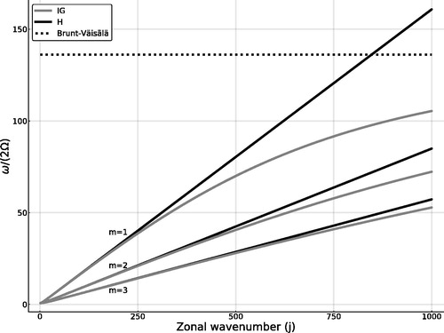
shows the dispersion curves of inertio-acoustic and inertio-gravity waves associated with the meridional wavenumber n = 1, for the first three baroclinic modes m = 1, 2, 3. shows the eastward branch of both wave types. To highlight the non-hydrostatic effect on the inertio-gravity waves, displays only the inertio-gravity wave dispersion curves associated with the meridional wavenumber n = 1 and the first three baroclinic modes, together with the corresponding dispersion curves obtained with hydrostatic approximation. The eigenfrequency of hydrostatic inertio-gravity waves is obtained by determining the equivalent height He from the simplified version of Equationequation (16)(16)
(16) for
and then computing the eigenfrequency by the well-known shallow-water equation dispersion relation
shows that the non-hydrostatic effect on the inertio-gravity waves only becomes noticeable for zonal wavenumbers j > 400 (
). An important point to be observed in is that, for a discrete spectrum of vertical eigenmodes resulting from a finite top zT in Equationequation (18)
(18)
(18) , there is a large time-scale separation between inertio-acoustic and inertio-gravity modes. This high time–frequency separation increases for higher vertical wavenumbers and has important consequences for the nature of the non-linear interactions between these wave types. For example, this time–frequency separation prevents an acoustic mode to be unstable to a pair of gravity wave modes in a single triad interaction, as it will be shown in Section 4.
Fig. 1. Dispersion curves of inertia-acoustic (AI) and inertia-gravity (IG) waves corresponding to the first three baroclinic modes m = 1, 2, 3. All the curves are referred to the meridional index n = 1.
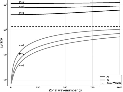
Fig. 2. Similar to , but only for the inertia-gravity waves (IG) and their corresponding dispersion curves obtained by hydrostatic approximation (H).
The exact conservation of given by Equationequation (11a)
(11a)
(11a) in the linear case implies that the linear eigenmodes satisfy the following orthogonality relation (Kasahara and Qian, Citation2000; Qian and Kasahara, Citation2003):
(22)
(22)
where
and
represent two arbitrary eigenvectors whose components are defined by equation (Equation12
(12a)
(12a) ) and
refers to the inner product in terms of pseudo-energy
given by
with the superscript ‘*’ indicating the complex conjugate.
3. General solution
3.1. Modal expansion
Now we use the orthogonality and completeness of the linear eigenmode functions described in the previous section to expand the solution of our nonlinear system Equation(1)–(5) in a series
(23)
(23)
where ‘C.C.’ indicates the complex conjugate of what is preceding,
refers to the complex-valued spectral amplitudes and the vector
represents the eigenvector function of a particular mode given by equation (Equation12
(12a)
(12a) ). Expansion series above is an exact solution of system Equation(1)–(5) provided the mode amplitudes Aa satisfy
(24)
(24)
In Equationequation (24)(24)
(24) ,
is the intrinsic energy (i.e. the squared norm) of the a-th mode and
represents the mismatch among the linear eigenfrequencies of each mode triplet abc. If
the triad is said to be resonant; the coupling constants
are the projection of the non-linear terms due to the action of two modes b and c onto another mode a, viz.,
(25)
(25)
where
is the bilinear operator containing the non-linear terms of system Equation(1)–(5), and hence all the information on the non-linearity of our model equations is contained in these coefficients. The interacting triads are those whose coupling constants are non-zero. The orthogonality of the (x, y) basis functions
requires the wave modes of an interacting triad to satisfy
(26a)
(26a)
(26b)
(26b)
In contrast, the vertical coupling integrals involved in Equationequation (25)(25)
(25) appear in the form
Thus, due to the presence of the ‘weight function’ in the vertical coupling constants, unlike the horizontal wavenumbers, there is no an excluding selection rule imposed by the vertical structures of the triad components. However, as ρ0 is a monotonically decreasing function of z, if
the vertical coupling integrals will be small, so that the triads whose wave modes do satisfy the condition
(27)
(27)
together with conditions Equation(26)
(26a)
(26a) are believed to undergo the strongest interactions, although condition (Equation27
(27)
(27) ) is no longer excluding. However, this non-excluding nature of the vertical coupling integrals allows a triad of modes whose vertical wavenumbers do not satisfy condition (Equation27
(27)
(27) ) to be excited by a primary triplet that does so, as it will be shown in the next section. Therefore, hereafter we will assume only the condition (Equation26
(26a)
(26a) ) to be met when referring to interacting triads.
3.2. Energy constraints for the interacting triads
As explained by Ripa (Citation1981) in the context of barotropic Rossby waves and internal gravity waves in a vertical plane and Ripa (Citation1983a) and Vanneste and Vial (Citation1994) for the equatorial beta-plane and spherical geometry shallow-water equations, respectively, the conserved quantities which are quadratic to lowest order in terms of wave disturbances lead to relations among the coupling constants of an interacting triad. Thus, in what follows we shall apply their approach in our non-hydrostatic context. In this way, substituting the mode expansion (Equation23(23)
(23) ) into Equationequations (11a)
(11a)
(11a) and (11 b) yields:
(28a)
(28a)
(28b)
(28b)
Equations above show that, as a consequence of the orthogonality relation (Equation22(22)
(22) ), the leading-order (quadratic) pseudo-energy has a diagonalised representation in terms of the linear eigenmodes, whereas the cubic energy
is expanded in terms of all interacting triads, with coefficients Sabc being given by
(29)
(29)
where CP means the same term as what is preceding but with cyclic permutations among the subscripts abc. On the other hand, from Equationequation (
(24)
(24) Equation24
(24)
(24) Equation)
(24)
(24) it follows
(30a)
(30a)
(30b)
(30b)
Taking the time derivative of Equationequations (28a,b)(28a)
(28a) and using equation (Equation30
(30a)
(30a) ) we get
(31)
(31)
Equation above shows that total pseudo-energy is no longer conserved for an arbitrary truncation of (Equation23(23)
(23) ).Footnote2 However, the rate of change of total pseudo-energy for an arbitrary truncation of our model equations is of
Thus, the smaller the disturbance amplitude the smaller the variation of total pseudo-energy for a truncated version of the model. Conversely, irrespective of the modal truncation, a necessary condition for Equationequation (31)
(31)
(31) to hold is that the sum inside the square brackets must vanish identically for all interacting triads, namely
(32)
(32)
For resonant triads () or triads containing only vortical modes, the constraint above reduces to
For these kinds of wave triplets, the quadratic component of total pseudo-energy is exactly conserved. Consequently, for these triads the coupling constants
and
have always the same sign, and the wave mode with the largest absolute value coupling constant (say, mode a) will always receive energy from or lose energy to the remaining triad components. Moreover, in these resonant interactions, condition
together with the resonance relation
implies that this mode having the largest absolute value coupling coefficient will always be the one with the largest absolute eigenfrequency. This mode is usually labeled as pump wave from the context of plasma physics (Weiland and Wilhelmsson, Citation1977). However, for non-resonant triads the pump mode, or the potentially unstable mode of the triad does not necessarily have the largest absolute coupling coefficient, according to relation (Equation32
(32)
(32) ).
Indeed, summarises a sample of interacting triads involving acoustic and gravity wave types. It can be noted that the acoustic mode is always the pump wave in near resonant triads involving acoustic and gravity modes (i.e. triads containing two acoustic modes and one gravity wave). In contrast, for interacting triads involving two gravity modes and one acoustic wave, which are characterised by a large frequency mismatch δabc, either an acoustic mode (e.g. Triads 3, 5 and 9) or an gravity wave (e.g. Triads 6, 7, 8, 14 and 15) can be the unstable mode (pump mode) of the triplet. However, the large time–frequency mismatch associated with this triad interaction type inhibits the energy exchanges among the mode components, since it requires an unrealistically high amplitude of the pump mode in order for instability to occur, as it will be shown in the next section.
Table 2. Representative examples of interacting triads involving inertia-acoustic (IA) and inertia-gravity modes (IG).
4. Analysis of highly truncated spectral solutions
Given the general theoretical framework on the non-linear interaction among the wave modes of our non-hydrostatic model employed in the previous section, in this section we will further investigate highly truncated versions of the interaction Equationequation (24)(24)
(24) to analyse the possibility of acoustic modes to excite inertio-gravity waves. First we will consider the most elementary form of the interaction equations: a single interacting wave triplet. Then we augment our analysis for considering two coupled interacting wave triads.
4.1. Single triad interaction
If one truncates the modal expansion (Equation23(23)
(23) ) to consider a single interacting triad of modes (a, b, c), Equationequation (24)
(24)
(24) now reads:
(33a)
(33a)
(33b)
(33b)
(33c)
(33c)
In the case of a resonant interaction (), it is well known that if one of the wave modes holds most part of the initial energy of the triplet, this mode will only be unstable if it is the pump wave of the triad (Craik, Citation1988, Chapter 8). Here, we extend such linear stability analysis for an arbitrary value of the mismatch δabc to encompass all the possibilities of interacting triads involving acoustic and gravity modes in this model.
To study the stability of one-wave mode in the single-triad interaction equations above, it is suitable to make the transformation of variable Inserting this transformation, Equationequations (33a,b,c)
(33a)
(33a) become
(34a)
(34a)
(34b)
(34b)
(34c)
(34c)
where the ‘
’ has been omitted to avoid cumbersome notation. Let us assume that Mode a holds almost the total energy of the triad initially, that is,
With this assumption, Equationequation (34)
(34a)
(34a) can be approximated by their linearized version around the amplitude of Mode a as follows
(35a)
(35a)
(35b)
(35b)
Thus, as the coupling constants are purely imaginary numbers, in order for instability to occur two conditions must be satisfied:
(36a)
(36a)
(36b)
(36b)
Otherwise, the solution is stable, and no amplification of Modes b and c occurs. Condition (36a) says that Mode a must be the pump mode of the triad. For an exact resonant interaction, this condition is the only requirement for instability to occur. Conversely, according to condition (36b), the minimal value of the amplitude of Mode a for instability to occur increases linearly as the absolute value of the mismatch parameter increases.
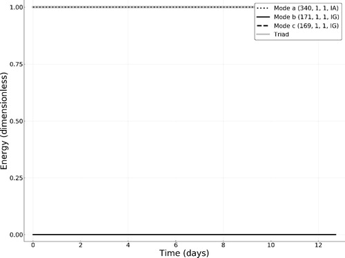
Consequently, for an interacting wave triplet composed of two inertio-gravity waves and one inertio-acoustic mode, the amplitude regime of the pump mode required to yield instability might be so high to be observable in the real atmosphere due to the high time–frequency mismatch among the triad components in this case. For example, for the case of Triad 3 of composed of mesoscale acoustic and gravity modes, the frequency mismatch is giving a threshold amplitude associated with vertical wind perturbations of the order of 200 m/s. Thus, for an acoustic mode amplitude value yielding dynamical field perturbations with realistic values, there is no pump wave instability for this triplet. shows the result of a time integration of the full nonlinear version of the three-wave interaction Equationequation (33)
(33a)
(33a) for an amplitude value of the pump mode of Triad 3 of that yields realistic values of the perturbation field variables. confirms that, for the mode amplitudes associated with realistic values of atmospheric flow disturbances, the high-frequency mismatch associated with the interacting triads involving an acoustic mode and two gravity waves strongly inhibits the energy exchanges among the modes of such triads.
Fig. 3. Time evolution of the mode quadratic energies associated with the solution of the three-wave interaction Equationequations (33)(33a)
(33a) for the modes of Triad 3 of . The present triad is non-resonant.
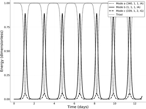
In contrast, an acoustic-inertia wave mode can undergo pump wave instability in near resonant triads involving another acoustic-inertia wave and an inertio-gravity mode. In fact, for the parameters of Triad 1 of and the value of chosen to yield a vertical wind magnitude of
m/s, parametric instability does occur. Numerical integration of the full Equationequation (33)
(33a)
(33a) in this referred amplitude regime illustrates the expressive energy modulations undergone by the three-wave modes () of this triplet.
Fig. 4. Time evolution of the mode quadratic energies associated with the solution of the three-wave interaction Equationequations (33)(33a)
(33a) for the modes of Triad 1 of . The present triad is nearly resonant.
Raupp et al. (Citation2019) analysed the dynamics of a single resonant triad interaction with a wave triplet similar to the one illustrated in . They analysed the analytical solution of the interaction Equationequation (33)(33a)
(33a) for the exact resonant case
with
and discussed the consequences of the mode energy modulations for the physical space solution
in view of the energy partition of each mode type on the kinetic, available elastic and available potential forms. Here we will not repeat this analysis and, rather, will stick to the modal space dynamics to further investigate the possibility of an acoustic mode to excite inertio-gravity waves. As in the full system (Equation24
(24)
(24) ) a single-wave mode may participate of several connected wave triplets, to investigate in a simplified fashion the possibility of each of the wave modes excited by the pump acoustic wave instability shown in to excite other gravity wave modes, we shall augment our analysis of the phase-space dynamics to consider two triads coupled by a single mode.
4.2. Two triads coupled by one mode
Let us now consider a truncated version of modal expansion (Equation23(23)
(23) ) that considers five modes (a,b,c,d,e) whose wavenumbers and eigenfrequencies satisfy the relations
(37a)
(37a)
(37b)
(37b)
(37c)
(37c)
(37d)
(37d)
(37e)
(37e)
(37f)
(37f)
(37g)
(37g)
Notice that we have imposed the interaction condition for the vertical wavenumbers only to the primary triad (a,b,c). This is because the condition for the vertical wavenumbers is no longer excluding, as previously discussed, so that other modes whose coupling constants are non-zero, although small, can be excited by the mode coupling the two triads. In this situation, Equationequation ((24)
(24) Equation24
(24)
(24) Equation)
(24)
(24) now reads
(38a)
(38a)
(38b)
(38b)
(38c)
(38c)
(38d)
(38d)
(38e)
(38e)
Thus, to analyse the stability of the triad interaction (a,b,c) to small amplitude perturbations associated with the interacting modes (c,d,e), let us first assume that In this case, Mode c evolves independently of Modes d and e, and its amplitude obeys the three-wave Equationequations (33)
(33a)
(33a) . Furthermore, by explicitly expressing Ac, Ad and Ae in terms of their real and imaginary parts, the linearized version of Equationequation (38d
(38d)
(38d) ,e) around the amplitude of Mode c can be written as
(39)
(39)
where
and the matrix M(t) is defined by
(40)
(40)
with
being defined as
(41)
(41)
If the matrix coefficient M(t) is periodic, Floquet theorem (Arnol’d, Citation1989; Vanneste and Vial, Citation1994; Majda, Citation2003) can be used to study the stability of system (Equation39(39)
(39) ). Conversely, as we are considering arbitrary time–frequency mismatchs δabc and δcde, in order for M(t) to be exactly periodic (and, therefore, Floquet theory be applicable), two conditions must be met: (i) the mismatch δabc and the non-linear oscillation frequency of the spectral amplitudes Aa, Ab and Ac must be co-measurable; and (ii) the resulting oscillation frequency of
be also co-measurable with the second triad mismatch δcde. As these two conditions are very restrictive, a more general way to analyse the stability of the aforementioned linear system is to estimate its maximal Lyapunov exponent (MLE) (Zounes and Rand, Citation1998), for which the MLE being positive means instability.Footnote3 The MLE has been evaluated using the method described in Benettin et al. (Citation1976), whose implementation is available in (Datseris, Citation2018).
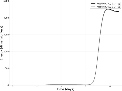
For the five-wave system composed of the modes of Triads 1 and 2 of , the MLE of system (Equation39(39)
(39) ) associated with the linearised dynamics of the gravity modes (170, 1, 2) and (169, 1, 2) is
corresponding to a growth rate of
which seems compatible with the typical time scale of internal-gravity waves. In this case, the time modulation of
refers to the solution shown in . The instability of the gravity wave-mode (339, 1, 2) to the other two gravity modes of Triad 2 of is illustrated in the numerical integration of system (Equation39
(39)
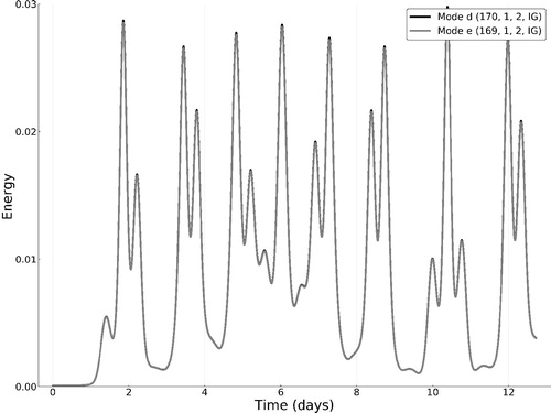
(39) ) shown in , which shows the growth of the gravity wave harmonics (170, 1, 2) and (169, 1, 2). Since the gravity mode (339, 1, 2) representing Mode c in this example is the pump wave of the triplet (c,d,e), this instability appears more likely to be a pump wave instability than a modulational instability explored by Connaughton et al. (Citation2010) in the Rossby wave context.
Fig. 5. Numerical solution of the linearized system (39) composed of modes (170,1,2,IG) and (169,1,2,IG) of Triad 2. These modes are parametrically forced by the mode (339, 1, 2, IG) of Triad 1. This solution presents a maximal Lyapunov exponent
In fact, if we consider the coupling between Triads 1 and 13 of through the same gravity mode (339, 1, 2), that is, if we replace Triad 2 to Triad 13 (which has a larger time–frequency mismatch) in our five-wave system, the solution of (Equation39(39)
(39) ) is stable (MLE
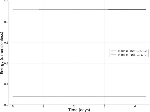
) and no amplification of a pair of other gravity waves occurs (). shows a similar situation when Modes d and e are gravity modes and Mode c is an inertio-acoustic mode. In this case, the planetary acoustic mode of Triad 1 of couples this triad with the two inertio-gravity modes of Triad 15, and the MLE of system (Equation39
(39)
(39) ) is positive but very close to zero. In fact, the MLE in this case is
corresponding to a growth rate of
which is no longer compatible with the observed time scale of gravity waves. Therefore, in this situation, as in the previous case shown in , system (Equation39
(39)
(39) ) is stable and there is no amplification of the two gravity modes. The numerical integration of the non-linear five-wave system (Equation38
(38a)
(38a) ) for the corresponding stable cases of the linearized system (Equation39
(39)
(39) ) shown in and confirms that there is no energy leakage from Triad 1 towards the other gravity modes, so that the time evolution of Modes (a,b,c) is identical to that predicted by the three-wave problem shown in (figures not shown).
Fig. 6. Numerical solution of the linearized system (39) composed of modes (170,1,1,IG) and (169,1,1,IG) of Triad 13. These modes are parametrically forced by the mode (339, 1, 2, IG) of Triad 1. This solution presents a maximal Lyapunov exponent
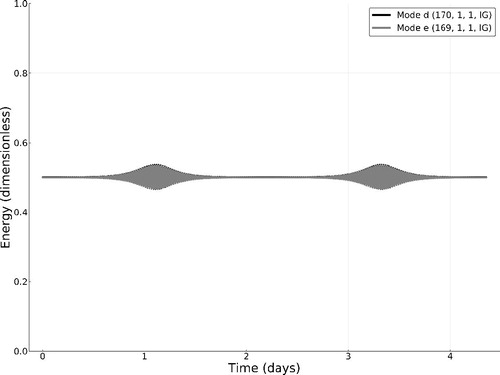
Fig. 7. Numerical solution of the linearized system (39) composed of modes (169,1,2,IG) and (–168,1,1,IG) of Triad 15. These modes are parametrically forced by the mode (1, 1, 1, IA) of Triad 1. This solution presents a maximal Lyapunov exponent
A result of numerical integration of the full five-wave system for the unstable case of system (Equation39(39)
(39) ) is shown in and . In this numerical integration, the initial condition is similar to those considered in , in which the pump acoustic wave (340, 1, 1) holds almost total initial energy of the system, with only a small perturbation distributed among the remaining modes b, c, d and e. From and one notices that, after Mode a excites Modes b and c through pump wave instability, part of Mode c energy leaks to the gravity modes (170, 1, 2) and (169, 1, 2) (Modes d and e), yielding the excitation of these modes. In this case, Mode c acts as the pump mode in the triad interaction with Modes d and e. Consequently, the time evolution of the mode energies of the five-wave system in this case shows that, apart from the considerable energy modulations of the gravity modes d and e at the expense of Mode c, the coupling of Mode c with the two gravity modes d and e also yields a multiplication of the periods associated with the time evolution of the energies of Modes a and b, disturbing the energy modulations of these modes from their exactly periodic nature predicted by the three-wave Equationequations (33)
(33a)
(33a) .
Fig. 8. Numerical solution of the five-wave system (38) composed of the modes of Triads 1 and 2 of . This figure illustrates the time evolution of the quadratic energies corresponding to Modes of Triad 1 only.
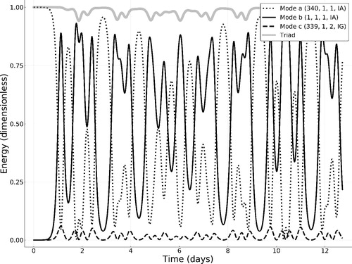
Fig. 9. This is same as , but illustrating the quadratic energies of the secondary gravity modes of Triad 2.
Another interesting feature regarding the unstable case is that the eigenfrequencies of the gravity modes (170, 1, 2) and (169, 1, 2) representing Modes d and e in this example are such that the linear wave dynamics of these modes is well described by hydrostatic approximation, as well as the non-linear interaction involving these inertio-gravity waves and vortical modes. As the non-linear interaction involving inertio-gravity waves and vortical modes has been demonstrated to play an important role in the non-linear geostrophic adjustment (Majda and Embid, Citation1998; Vanneste, Citation2004; Vanneste and Yavneh, Citation2004), the theoretical results described here suggest that acoustic modes might be important for both hydrostatic and geostrophic adjustment processes in the atmosphere.
5. Summary and conclusions
Non-linear triad interactions involving inertio-acoustic and inertio-gravity waves are studied here in the context of the mid-latitude f-plane shallow non-hydrostatic equations for a background state at rest and characterised by a hydrostatic balance and an isothermal temperature profile. In this context, we have adopted highly truncated Galerkin expansions in terms of the eigensolutions of the linear problem. For a single-triad interaction, we have shown that the interacting triplets involving two inertio-gravity waves and one acoustic mode require a likely unrealistic modal amplitude regime in order for pump wave instability to occur. Consequently, for direct triad interactions, we have shown that an inertio-acoustic wave mode can only be unstable to perturbations associated with a pair of acoustic/gravity modes.
In contrast, the analysis of the dynamics of two triads coupled by a single-wave mode shows that a non-hydrostatic inertio-gravity wave mode (i.e. having an eigenfrequency such that the non-hydrostatic effect of vertical acceleration is not negligible) participating of a nearly resonant interaction with two acoustic modes is unstable in nearly resonant triad interactions with a pair of lower frequency inertio-gravity waves. In fact, for the representative example illustrated here in which the eigenfrequencies of the two excited inertio-gravity waves are nearly a half of the time–frequency of the primary wave (which couples the two triads), the numerical results of the non-linear dynamics of the five-wave system confirm that this instability yields energy modulations on the two secondary gravity modes. Since the higher the time frequency the more important the non-hydrostatic effect of vertical acceleration on the inertio-gravity waves, the results suggest that inertio-acoustic waves may induce hydrostatically balanced inertio-gravity waves to undergo episodic amplitude (energy) modulations due to inter-triad energy exchanges. On the other hand, if one of the acoustic modes of a resonant interaction involving acoustic/gravity waves couple the two triads in our reduced five-wave dynamics, our results show that the maximum Lyapunov exponent of the corresponding linearized system for the two gravity waves gives a growth time-scale of days, which is no longer compatible with the observed time-scale of internal gravity waves and, consequently, the resulting instability might likely be irrelevant in the atmosphere.
As discussed in Section 1, due to the ultra-high frequency of acoustic waves, their numerical treatment using explicit schemes implies highly restrictive computational constraints. Consequently, in non-hydrostatic numerical models adopted for meso-scale simulations the acoustic modes are either filtered out or subjected to strong damping associated with implicit schemes having time-steps much higher than the acoustic cut-off period. However, acoustic waves play an important role in the hydrostatic adjustment process as they are responsible for the vertical displacements of fluid parcels associated with the expansion of an instantaneously heated atmospheric layer (Bannon, Citation1995, Citation1996; Duffy, Citation2003). In fact, Chagnon and Bannon (Citation2001) demonstrated that the steady-state solutions of anelastic and other sound filtering models exhibit significant differences from those of fully compressible models allowing acoustic modes.
Acoustic waves may be excited by thermal forcings associated with convective storms, especially the localized ones that have a duration shorter than the acoustic cut-off period given by (Chagnon and Bannon, Citation2005a, Citation2005b). Our simplified theoretical model suggests that these acoustic modes generated by explosive and localised storms might play an important role in the transient phase of the three-dimensional adjustment process of the atmosphere to both hydrostatic and geostrophic balances. Specifically, this role of acoustic modes in the adjustment process of the atmosphere might be due to not only their linear energy propagation as studied by Chagnon and Bannon (Citation2005a, Citation2005b) but also their non-linear effect of exciting hydrostatic inertio-gravity waves as pointed out by our theoretical analysis. Fanelli and Bannon (Citation2005) investigated the hydrostatic and geostrophic adjustments to a prescribed thermal forcing utilising a non-linear compressible model, but they considered a heating function with a duration longer than the acoustic cut-off period of
min so that no acoustic waves were excited. However, similar numerical studies with a shorter time-scale forcing should be done to apply this theory to the hydrostatic and geostrophic adjustments in a more realistic fashion by considering the full expansion (Equation23
(23)
(23) ). This might be the next step in the generalisation of this theory to further understand both the non-linear dynamics of the non-hydrostatic wave modes itself and its role in the non-linear hydrostatic/geostrophic adjustment, along with testing the robustness of this theory.
Acknowledgements
The authors thank Dr. Breno Raphaldini and Dr. David Ciro Taborda for their helpful suggestions. The authors also acknowledge the insightful and constructive comments of the anonymous reviewer.
Disclosure statement
No potential conflict of interest was reported by the authors.
Additional information
Funding
Notes
1 r = 0 for a vortical mode and (±2) for westward/eastward inertio-gravity (inertio-acoustic) modes, for example.
2 In reality, total pseudo-energy of model Equationequations (1)–(5) is not exactly conserved even for the full expansion case due to the terms in Equationequation (10)
(10)
(10) .
3 To estimate the MLE (ΛL) of we obtain two solutions whose initial conditions differ by a small separation, namely
and
with
Then, the MLE is defined by the following equation
representing a measure of the exponential rate of separation between two neighbouring trajectories.
References
- Andrews, D. G. 1981. A note on potential energy density in a stratified compressible fluid. J. Fluid Mech. 107, 227–236. doi:10.1017/S0022112081001754
- Arnol’d, V. 1989. Mathematical Methods of Classical Mechanics. Graduate Texts in Mathematics. Springer, New York.
- Bannon, P. R. 1995. Hydrostatic adjustment: Lamb’s problem. J. Atmos. Sci. 52, 1743–1752. doi:10.1175/1520-0469(1995)052<1743:HALP>2.0.CO;2
- Bannon, P. R. 1996. Nonlinear hydrostatic adjustment. J. Atmos. Sci. 53, 3606–3617. doi:10.1175/1520-0469(1996)053<3606:NHA>2.0.CO;2
- Benettin, G., Galgani, L. and Strelcyn, J.-M. 1976. Kolmogorov entropy and numerical experiments. Phys. Rev. A 14, 2338–2345. doi:10.1103/PhysRevA.14.2338
- Bustamante, M. D., Quinn, B. and Lucas, D. 2014. Robust energy transfer mechanism via precession resonance in nonlinear turbulent wave systems. Phys. Rev. Letters. 113, 084502. doi:10.1103/PhysRevLett.113.084502
- Chagnon, J. M. and Bannon, P. R. 2001. Hydrostatic and geostrophic adjustment in a compressible atmosphere: Initial response and final equilibrium to an instantaneous localized heating. J. Atmos. Sci. 58, 3776–3792. doi:10.1175/1520-0469(2001)058<3776:HAGAIA>2.0.CO;2
- Chagnon, J. M. and Bannon, P. R. 2005a. Wave response during hydrostatic and geostrophic adjustment. Part I: Transient dynamics. J. Atmos. Sci. 62, 1311–1329. doi:10.1175/JAS3283.1
- Chagnon, J. M. and Bannon, P. R. 2005b. Wave response during hydrostatic and geostrophic adjustment. Part II: Potential vorticity conservation and energy partitioning. J. Atmos. Sci. 62, 1330–1345. doi:10.1175/JAS3419.1
- Connaughton, C., Nadiga, B. T., Nazarenko, S. and Quinn, B. 2010. Modulational instability of Rossby and drift waves and generation of zonal jets. J. Fluid Mech. 654, 207–231. doi:10.1017/S0022112010000510
- Craik, A. D. D. 1988. Wave interactions and fluid flows. Cambridge Monographs on Mechanics and Applied Math. Cambridge University Press, Cambridge, UK.
- Daley, R. 1988. The normal modes of the spherical nonhydrostatic equations with applications to the filterinf of acoustic modes. Tellus 40A, 96–106. doi:10.1111/j.1600-0870.1988.tb00409.x
- Datseris, G. 2018. Dynamicalsystems.jl: A Julia software library for chaos and nonlinear dynamics. JOSS. 3, 598. doi:10.21105/joss.00598
- Davies, T., Staniforth, A., Wood, N. and Thuburn, J. 2003. Validity of anelastic and other equation sets as inferred from normal-mode analysis. Q. J. R. Meteorol. Soc. 129, 2761–2775. doi:10.1256/qj.02.1951
- Domaracki, A. and Lossch, A. Z. 1977. Nonlinear interactions among equatorial waves. J. Atmos. Sci. 34, 486–498. doi:10.1175/1520-0469(1977)034<0486:NIAEW>2.0.CO;2
- Duffy, D. G. 1974. Resonant interactions of inertio-gravity and Rossby waves. J. Atmos. Sci. 31, 1218–1231. doi:10.1175/1520-0469(1974)031<1218:RIOIGA>2.0.CO;2
- Duffy, D. G. 2003. Hydrostatic adjustment in nonisothermal atmospheres. J. Atmos. Sci. 60, 339–353. doi:10.1175/1520-0469(2003)060<0339:HAINA>2.0.CO;2
- Eckart, C. 1960. Hydrodynamics of Oceans and Atmospheres. Pergamon Press, London.
- Fanelli, P. F. and Bannon, P. R. 2005. Nonlinear atmospheric adjustment to thermal forcing. J. Atmos. Sci. 62, 4253–4272. doi:10.1175/JAS3517.1
- Giraldo, F. X., Restelli, M. and Läuter, M. 2010. Semi-implicit formulations of the Navier-Stokes equations: Application to nonhydrostatic atmospheric modeling. SIAM J. Sci. Comput. 32, 3394–3425. doi:10.1137/090775889
- Janssen, P. A. E. M. 2003. Nonlinear four-wave interactions and freak waves. J. Phys. Oceanogr. 33, 863–884. doi:10.1175/1520-0485(2003)33<863:NFIAFW>2.0.CO;2
- Kasahara, A. 2003a. The roles of the horizontal component of the earth’s angular velocity in nonhydrostatic linear models. J. Atmos. Sci. 60, 1085–1095. doi:10.1175/1520-0469(2003)60<1085:TROTHC>2.0.CO;2
- Kasahara, A. 2003b. On the nonhydrostatic atmospheric models with inclusion of the horizontal component of the earth’s angular velocity. JMSJ. 81, 935–950. doi:10.2151/jmsj.81.935
- Kasahara, A. 2004. Free oscillations of deep nonhydrostatic global atmospheres: Theory and a test of numerical schemes. NCAR Tech. Rep. NCAR/TN-457 + STR, NCAR. University Corporation for Atmospheric Research, Boulder, CO.
- Kasahara, A. and Gary, M. 2006. Normal modes of an incompressible and stratified fluid model including the vertical and horizontal components of Coriolis force. Tellus 58, 368–384. doi:10.1111/j.1600-0870.2006.00182.x
- Kasahara, A. and Qian, J.-H. 2000. Normal modes of a global nonhydrostatic atmospheric model. Mon. Wea. Rev. 128, 3357–3375. doi:10.1175/1520-0493(2000)128<3357:NMOAGN>2.0.CO;2
- Klein, R. 2009. Asymptotics, structure, and integration of sound-proof atmospheric flow equations. Theor. Comput. Fluid Dyn. 23, 161–195. doi:10.1007/s00162-009-0104-y
- Klemp, J. B., Skamarock, W. C. and Ha, S. 2018. Damping acoustic modes in compressible horizontally explicit vertically implicit (HEVI) and split-explicit time integration schemes. Mon. Wea. Rev. 146, 1911–1923. doi:10.1175/MWR-D-17-0384.1
- Loesch, A. Z. and Deininger, R. C. 1979. Dynamics of closed systems of resonantly interacting equatorial waves. J. Atmos. Sci. 36, 1490–1497. doi:10.1175/1520-0469(1979)036<1490:DOCSOR>2.0.CO;2
- Majda, A. 2003. Introduction to PDEs and Waves for the Atmosphere and Ocean. Courant Lecture Notes in Mathematics Series. Courant Institute of Mathematical Sciences,.New York University, New York.
- Majda, A. J. and Embid, P. 1998. Averaging over fast waves for geophysical flows with unbalanced initial data. Theor. Comput. Fluid Dyn. 11, 155–169. doi:10.1007/s001620050086
- Pielke, R. 2002. Mesoscale Meteorological Modeling. International Geophysics Series. Academic Press, California. ISBN 9780125547666.
- Qian, J.-H. and Kasahara, A. 2003. Nonhydrostatic atmospheric normal modes on beta-planes. Pure Appl. Geophys. 160, 1315–1358.
- Raupp, C. F. M., Silva Dias, P. L., Tabak, E. G. and Milewski, P. 2008. Resonant wave interactions in the equatorial waveguide. J. Atmos. Sci. 65, 3398–3418. doi:10.1175/2008JAS2387.1
- Raupp, C. F. M., Teruya, A. S. W. and Silva Dias, P. L. 2019. Linear and weakly nonlinear energetics of global nonhydrostatic normal modes. J. Atmos. Sci. 76, 3831–3846. doi:10.1175/JAS-D-19-0131.1
- Ripa, P. 1981. On the theory of nonlinear wave-wave interactions among geophysical waves. J. Fluid Mech. 103, 87–115. doi:10.1017/S0022112081001250
- Ripa, P. 1983a. Weak interactions of equatorial waves in a one-layer model. Part I: General properties. J. Phys. Oceanogr. 13, 1208–1226. doi:10.1175/1520-0485(1983)013<1208:WIOEWI>2.0.CO;2
- Ripa, P. 1983b. Weak interactions of equatorial waves in a one-layer model. Part II: Applications. J. Phys. Oceanogr. 13, 1227–1240. doi:10.1175/1520-0485(1983)013<1227:WIOEWI>2.0.CO;2
- Shepherd, T. D. 1990. Symmetries, conservation laws, and Hamiltonian structure in geophysical fluid dynamics. Adv. Geophys. 32, 287–338. doi:10.1016/S0065-2687(08)60429-X
- Shepherd, T. G. 1993. A unified theory of available potential energy. Atmos. Ocean 31, 1–26. doi:10.1080/07055900.1993.9649460
- Smith, L. M. and Lee, Y. 2005. On near resonances and symmetry breaking in forced rotating flows at moderate Rossby number. J. Fluid Mech. 535, 111–142. doi:10.1017/S0022112005004660
- Taylor, G. I. 1936. The oscillations of the atmosphere. Proc. R. Soc. London 156, 318–326.
- Thuburn, J. 2011. Some basic dynamics relevant to the design of atmospheric model dynamical cores. In: Numerical Techniques for Global Atmospheric Models (eds. P. H. Lauritzen, C. Jablonowski, M. A. Taylor and R. D. Nair) Vol. 80, Chapter 1, Springer, Berlin, pp. 3–27.
- Tribbia, J. 1979. Non-linear initialization on an equatorial beta-plane. Mon. Wea. Rev. 107, 704–713. doi:10.1175/1520-0493(1979)107<0704:NIOAEB>2.0.CO;2
- Vanneste, J. 2004. Inertia-gravity wave generation by balanced motion: revisiting the Lorenz-Krishnamurthy model. J. Atmos. Sci. 61, 224–234. doi:10.1175/1520-0469(2004)061<0224:IWGBBM>2.0.CO;2
- Vanneste, J. and Vial, F. 1994. Nonlinear wave propagation on a sphere: Interaction between Rossby waves and gravity waves; stability of the Rossby waves. Geophys. Astrophys. Fluid Dyn. 76, 121–144. doi:10.1080/03091929408203662
- Vanneste, J. and Yavneh, I. 2004. Exponentially small inertia-gravity waves and the breakdown of quasigeostrophic balance. J. Atmos. Sci. 61, 211–223. doi:10.1175/1520-0469(2004)061<0211:ESIWAT>2.0.CO;2
- Weiland, J. and Wilhelmsson, H. 1977. Coherent Nonlinear Interaction of Waves in Plasmas. Pergamon, Oxford; Turkey.
- White, A. A., Hoskins, B. J., Roulstone, I. and Staniforth, A. 2005. Consistent approximate models of the global atmosphere: Shallow, deep, hydrostatic, quasi-hydrostatic and non-hydrostatic. Q. J. R. Meteorol. Soc. 131, 2081–2107. doi:10.1256/qj.04.49
- Zounes, R. and Rand, R. 1998. Transition curves for the quasi-periodic Mathieu equation. SIAM J. Appl. Math. 58, 1094–1115. doi:10.1137/S0036139996303877