The extratropical transition of Hurricane Ophelia (2017) as diagnosed with a generalized omega equation and vorticity equation

Abstract

Hurricane Ophelia was a category 3 hurricane which underwent extratropical transition and made landfall in Europe as an exceptionally strong post-tropical cyclone in October 2017. In Ireland, Ophelia was the worst storm in 50 years and resulted in significant damage and even loss of life. In this study, the different physical processes affecting Ophelia’s transformation from a hurricane to a mid-latitude cyclone are studied. For this purpose, we have developed software that uses OpenIFS model output and a system consisting of a generalized omega equation and vorticity equation. By using these two equations, the atmospheric vertical motion and vorticity tendency are separated into the contributions from different physical processes: vorticity advection, thermal advection, friction, diabatic heating, and the imbalance between the temperature and vorticity tendencies. Vorticity advection, which is often considered an important forcing for the development of mid-latitude cyclones, is shown to play a small role in the re-intensification of the low-level cyclone. Instead, our results show that the adiabatic upper-level forcing was strongly amplified by moist processes, and thus, the diabatic heating was the dominant forcing in both the tropical and extratropical phases of Ophelia. Furthermore, we calculated in more detail the diabatic heating contributions from different model parameterizations. We find that the temperature tendency due to the convection scheme was the dominant forcing for the vorticity tendency during the hurricane phase, but as Ophelia transformed into a mid-latitude cyclone, the microphysics temperature tendency, presumably dominated by large-scale condensation, gradually increased becoming the dominant forcing once the transition was complete. Temperature tendencies caused by other diabatic processes, such as radiation, surface processes, vertical diffusion, and gravity wave drag, were found to be negligible in the development of the storm.

Keywords:

• extratropical transition
• hurricane
• omega equation
• vorticity tendency

1. Introduction

Tropical cyclones which curve poleward and enter mid-latitudes often lose their tropical characteristics and transform into mid-latitude cyclones through a process called extratropical transition (ET; Sekioka, 1956; Palmén, 1958). The ET does not occur instantly, but is rather defined as a time period during which the tropical characteristics of the cyclone are replaced by the features typical for mid-latitude cyclones, such as a cold core and fronts (e.g. Evans et al., 2017). An objective and widely used methodology to characterize the transformation process is the cyclone phase space diagram (Hart, 2003). The diagram describes both the thermal wind ($-V_T^L$-parameter) and frontal asymmetry (B-parameter) during the cyclone’s life cycle. Evans and Hart (2003) defined the onset of ET when the cyclone becomes asymmetric (B > 10 m) and the completion of ET when the cold core develops ($-V_T^L$ < 0 m).

In the North Atlantic, up to half of all tropical cyclones undergo ET and become mid-latitude cyclones (Hart and Evans, 2001; Bieli et al., 2019). Furthermore, out of the tropical cyclones that undergo extratropical transition in the North Atlantic, 51% undergo post-ET intensification (Hart and Evans, 2001). This result is based on a dataset covering 61 cases between 1979 and 1993. Thus, according to the climatology, western Europe is impacted by a transitioning tropical cyclone once every 1–2 years (Hart and Evans, 2001). These post-tropical storms can cause severe damage by themselves (e.g. Browning et al., 1998; Thorncroft and Jones, 2000; Feser et al., 2015), or downstream via amplification of the mid-latitude flow (Grams and Blumer, 2015; Keller et al., 2018). Moreover, due to the warming of climate, post-tropical storms impacting Europe are projected to become more frequent (Haarsma et al., 2013; Baatsen et al., 2015; Liu et al., 2017).

For this reason, understanding the atmospheric forcing mechanisms that cause tropical cyclones to intensify as post-tropical cyclones is of great importance. The energy source of tropical cyclones is the warm sea surface temperatures, which allow latent heat release via deep, moist convection. Extratropical cyclones are, in contrast, primarily driven by baroclinic processes due to meridional temperature and moisture gradients at mid-latitudes. Therefore, the ET of tropical cyclones involves often complex dynamics as the tropical storm enters the mid-latitudes and starts to experience the baroclinic environment.

The complexity of dynamics and the strong involvement of both thermodynamic and dynamic processes in the transitioning cyclones raises a relevant question: What is the relative importance of different forcing mechanisms for the cyclone during its transition process? This paper is a case study that attempts to answer this question by examining the contributions of different synoptic-scale forcing terms to the evolution of Hurricane Ophelia, which hit Ireland as a strong post-tropical storm in October 2017.

Earlier diagnostic case studies about extratropical cyclones have discovered the equal importance of diabatic heating and thermal advection to the Presidents’ Day cyclone in 1979 (Räisänen, 1997), the primary contribution from cyclonic vorticity advection to continental cool-season extratropical cyclones over the U.S. (Rolfson and Smith, 1996), and warm-air advection (diabatic heating) having the largest influence on explosive development in cold-core (warm-core) cyclones over the North Atlantic (Azad and Sorteberg, 2009). Bentley et al. (2019) studied the extratropical cyclones leading to extreme weather events over Central and Eastern North America. They concluded that both baroclinic and diabatic processes are important during the life cycles of the cyclones that lead to extreme weather. However, the study did not make an attempt to directly quantify the magnitude of the baroclinic and diabatic processes affecting the evolution of the cyclones. A very recent study (Seiler, 2019), performed with an inversion of potential vorticity, suggests that in about half of the extreme extratropical cyclones in the Northern Hemisphere the largest contribution to the maximum intensity is associated with condensational heating in the lower-level atmosphere.

There are numerous diagnostic studies about tropical cyclones that undergo extratropical transition in the literature. Milrad et al. (2009) studied poleward-moving tropical cyclones occurring in Eastern Canada during 1979–2005. According to their results, the differential vorticity advection above the surface cyclone played a major role in the post-ET intensification. The vorticity advection was associated with a decrease of the trough-ridge wavelength, which, in turn, led to a stronger circulation and larger values of warm-air advection. Consistently, the advection of vorticity by the non-divergent wind in the upper-troposphere was found to be a considerable forcing also for the reintensification of Tropical Storm Agnes along the East Coast of United States (DiMego and Bosart, 1982) and the extratropical cyclone developed from the remnants of Typhoon Bart in the Western North Pacific (Klein et al., 2002). Conversely, one reason for the post-tropical decay of Typhoon Jangmi in 2008 was its weak phasing with upper-level forcing for broad-scale ascending motion (Grams et al., 2013). Ritchie and Elsberry (2007) reported significantly stronger midtropospheric cyclonic vorticity advection and lower-tropospheric thermal advection above intensifying transitioning cyclones compared to the decaying ones. In summary, based on both real world examples and idealized simulations, there is clear evidence that baroclinic forcing terms can act substantially in the post-ET intensification.

We expect that diabatic processes were dominant in the tropical phase of Ophelia. We hypothesize also that that baroclinic processes became approximately as important as diabatic heating for the cyclone development when it moved to mid-latitudes and strengthened after the ET. In this study, the contributions of different forcing mechanisms to Ophelia’s evolution are assessed using a generalized omega equation and the vorticity equation. This equation system was adapted from Räisänen (1997), and the first version of the diagnostic software used in this paper was documented in Rantanen et al. (2017) (hereafter R17). The equations, the model simulation, and the diagnostic software are presented in Section 2. Section 3 provides the synoptic overview of Ophelia’s life cycle, and the performance of the model simulation is evaluated in Section 4. The main results, namely the contributions of different forcing terms to the atmospheric vertical motion and vorticity tendency of the cyclone, are presented in Section 5. Some aspects of the results are further discussed in Section 6, and finally, the main conclusions are given in Section 7.

2. Equations and model simulation

2.1. OpenIFS model and simulations

The life cycle of Ophelia was simulated with the Open Integrated Forecast System (OpenIFS) model, which is the open version of the Integrated Forecast System (IFS) model by the European Centre for Medium-Range Weather Forecasts (ECMWF). OpenIFS is not an open-source model, but available to academic and research institutions under licence.

IFS is a state-of-the-art global forecast model, which includes a data assimilation system and forecast systems for the atmosphere, ocean, waves, and sea ice. OpenIFS has only the atmospheric and wave model parts of the IFS, but contains exactly the same dynamics and physical parametrizations as IFS. OpenIFS does not have the data assimilation, so it can be used only for research purposes with externally generated initial conditions. The version of OpenIFS used in this study is cycle 40r1, which was in operational use at ECMWF from November 2013 to May 2015.

The initial conditions for the model simulations were generated from the ECMWF operational analyses. The model was run at a spectral resolution of T639, corresponding to 0.28125° × 0.28125° grid spacing, and with 137 model levels. One-hourly output was generated for 20 evenly spaced pressure levels, from 1000 hPa to 50 hPa. Some variables were also archived on constant potential vorticity and potential temperature levels. Coarser-resolution simulations with T159 and T255 spectral truncation were found to not capture the ET of Ophelia with sufficient accuracy (not shown).

The initialization time of the OpenIFS simulation was 12 UTC 13 October 2017. Ophelia developed into a hurricane at 18 UTC 11 October (Stewart, 2018). Model simulations with different initialization times, starting from 6 October to 16 October, were also examined. The runs with earlier initialization times, however, had larger errors in the track of Ophelia, and they also simulated the ET less accurately. The model simulations with later initialization times were mostly more accurate, but the length of the cyclone’s tropical phase in the simulation was shorter. Hence, the selected initialization time was a compromise between the skill of the forecast and the length of the simulation. The length of our simulation was six days, from which the first four days are examined in this paper.

2.2. ERA5 reanalysis

To verify that the transition of Ophelia was simulated correctly by OpenIFS, we compare the model output to reanalysis data. Reanalysis datasets are useful for analysing synoptic-scale weather systems, because reanalyses combine the available observational data with the model analysis, resulting in a consistent dataset over the years. For this study, we used ERA5 reanalysis from ECMWF. ERA5 covers the period from 1979 to present and has one-hourly temporal resolution with 31-km spatial grid spacing (T639 in spectral space). There are 137 levels from the surface up to a height of 80 km. ERA5 has been produced with a four-dimensional variational (4 D-Var) data assimilation system by the cycle 41r2 of ECMWF’s IFS model. ERA5 reanalysis data was downloaded from Copernicus Climate Data Store (cds.climate.copernicus.eu) for both pressure levels and the 2.0 potential vorticity unit (PVU) level for October 2017. The horizontal grid spacing of the ERA5 data was the same as in the OpenIFS model simulation. ERA5 alone is not used for this study as temperature and wind tendencies due to diabatic and frictional processes are not available for ERA5. These variables are required for our analysis and can be output from OpenIFS.

2.3. Equations

The equation system in this study consists of a generalized omega equation and the vorticity equation. The combination of these equations is adapted from Räisänen (1997).

2.3.1. Generalized omega equation and vorticity equation

The generalized omega equation is a diagnostic equation for analysing the causes of atmospheric vertical motions (Stepanyuk et al., 2017), which can be derived directly from the primitive equations in isobaric coordinates (Räisänen, 1995). The equation’s better-known form, the quasi-geostrophic (QG) omega equation, applies many assumptions such as use of geostrophic winds and omission of diabatic heating and friction. These simplifications in the QG omega equation markedly deteriorate its accuracy, and thus make it less useful for a detailed analysis of atmospheric vertical motions. By contrast, the generalized omega equation used in this study does not include any of the simplifications used in the QG theory, except for hydrostatic balance, which is always implicitly assumed when isobaric coordinates are used (Räisänen, 1995).

The generalized omega equation used here is the same as in R17: (1) $$L(\omega )=F_V+F_T+F_F+F_Q+F_A$$(1) where (2) $$L\left(\omega \right)={\nabla }^2\left(\sigma \omega \right)+f(\zeta +f)\frac{{\partial }^2\omega }{\partial p^2}-f\frac{{\partial }^2\zeta }{\partial p^2}\omega +f\frac{\partial }{\partial p}[\mathit{k}·(\frac{\partial \mathit{V}}{\partial p}\times \mathbf{\nabla }\omega )]$$(2) and the right-hand side (RHS) terms have the expressions (3) $$F_V=f\frac{\partial }{\partial p}\left[\mathit{V}·\mathbf{\nabla }\left(\zeta +f\right)\right],$$(3) (4) $$F_T=\frac{R}{p}{\nabla }^2\left(\mathit{V}·\mathbf{\nabla }T\right),$$(4) (5) $$F_F=-f\frac{\partial }{\partial p}\left[\mathit{k}·\left(\mathbf{\nabla }\times \mathit{F}\right)\right],$$(5) (6) $$F_Q=-\frac{R}{c_{p}p}{\nabla }^{2}Q,$$(6) (7) $$F_A=f\frac{\partial }{\partial p}\left(\frac{\partial \zeta }{\partial t}\right)+\frac{R}{p}{\nabla }^2\left(\frac{\partial T}{\partial t}\right).$$(7)

The symbols used in all the equations are listed in Table 1. The RHS terms of the equation represent the effects of different forcing mechanisms on vertical motion: differential vorticity advection (Eq. 3(3) $$F_V=f\frac{\partial }{\partial p}\left[\mathit{V}·\mathbf{\nabla }\left(\zeta +f\right)\right],$$(3) ), the Laplacian of thermal advection (Eq. 4(4) $$F_T=\frac{R}{p}{\nabla }^2\left(\mathit{V}·\mathbf{\nabla }T\right),$$(4) ), the curl of friction (Eq. 5(5) $$F_F=-f\frac{\partial }{\partial p}\left[\mathit{k}·\left(\mathbf{\nabla }\times \mathit{F}\right)\right],$$(5) ), and the Laplacian of diabatic heating (Eq. 6(6) $$F_Q=-\frac{R}{c_{p}p}{\nabla }^{2}Q,$$(6) ). The last term (Eq. 7(7) $$F_A=f\frac{\partial }{\partial p}\left(\frac{\partial \zeta }{\partial t}\right)+\frac{R}{p}{\nabla }^2\left(\frac{\partial T}{\partial t}\right).$$(7) ) describes the imbalance between temperature tendencies and vorticity tendencies. At mid-latitudes, and with constant R, the imbalance term (Eq. 7(7) $$F_A=f\frac{\partial }{\partial p}\left(\frac{\partial \zeta }{\partial t}\right)+\frac{R}{p}{\nabla }^2\left(\frac{\partial T}{\partial t}\right).$$(7) ) is proportional to the pressure derivative of ageostrophic vorticity tendency (Räisänen, 1995). The left-hand side (LHS) operator of the generalized omega equation (Eq. 2(2) $$L\left(\omega \right)={\nabla }^2\left(\sigma \omega \right)+f(\zeta +f)\frac{{\partial }^2\omega }{\partial p^2}-f\frac{{\partial }^2\zeta }{\partial p^2}\omega +f\frac{\partial }{\partial p}[\mathit{k}·(\frac{\partial \mathit{V}}{\partial p}\times \mathbf{\nabla }\omega )]$$(2) ) is linear with respect to ω. Hence, the contributions of the five RHS terms (Eqs. 3–7) can be solved separately provided that homogeneous boundary conditions (ω = 0 at the upper (p = 50 hPa) and lower (p = 1000 hPa) boundaries of the atmosphere) are used.

Table 1. List of mathematical symbols.

cp = 1004 J kg^−1	Specific heat of dry air at constant volume
f	Coriolis parameter
F	Forcing in the omega equation
F	Friction force per unit mass
k	Unit vector along the vertical axis
L	Linear operator on the left-hand-side of the omega equation
p	Pressure
ps	Surface pressure
Q	Diabatic heating rate per unit mass
R = 287 J kg^−1	Gas constant of dry air
t	Time
T	Temperature
V	Horizontal wind vector
${\mathit{V}}_{\chi }$	Divergent wind vector
${\mathit{V}}_{\psi }$	Rotational wind vector
χ	Velocity potential
ψ	Stream function
$\sigma =-\frac{RT}{p\theta }\frac{\partial \theta }{\partial p}$	Hydrostatic stability
ζ	Vertical component of relative vorticity
$\omega =\frac{dp}{dt}$	Isobaric vertical motion
$\mathbf{\nabla }$	Horizontal nabla operator
${\nabla }^2$	Horizontal Laplacian operator

By solving the generalized omega equation, and then using the vorticity equation (8) $$\frac{\partial \zeta }{\partial t}=-\mathit{V}\cdot \mathbf{\nabla }(\zeta +f)-\omega \frac{\partial \zeta }{\partial p}+(\zeta +f)\frac{\partial \omega }{\partial p}+\mathit{k}·\left(\frac{\partial \mathit{V}}{\partial p}\times \mathbf{\nabla }\omega \right)+\mathit{k}·\mathbf{\nabla }\times \mathit{F}$$(8) we can separate the atmospheric vertical motion (Eq. 9(9) $$\omega ={\omega }_V+{\omega }_T+{\omega }_F+{\omega }_Q+{\omega }_A$$(9) ) and vorticity tendency (Eq. 10(10) $$\frac{\partial \zeta }{\partial t}={\left(\frac{\partial \zeta }{\partial t}\right)}_V+{\left(\frac{\partial \zeta }{\partial t}\right)}_T+{\left(\frac{\partial \zeta }{\partial t}\right)}_F+{\left(\frac{\partial \zeta }{\partial t}\right)}_Q+{\left(\frac{\partial \zeta }{\partial t}\right)}_A.$$(10) ) fields into components caused by the five forcing terms: (9) $$\omega ={\omega }_V+{\omega }_T+{\omega }_F+{\omega }_Q+{\omega }_A$$(9) (10) $$\frac{\partial \zeta }{\partial t}={\left(\frac{\partial \zeta }{\partial t}\right)}_V+{\left(\frac{\partial \zeta }{\partial t}\right)}_T+{\left(\frac{\partial \zeta }{\partial t}\right)}_F+{\left(\frac{\partial \zeta }{\partial t}\right)}_Q+{\left(\frac{\partial \zeta }{\partial t}\right)}_A.$$(10)

Here the subscripts follow Eqs. 3–7. In Eq. 10(10) $$\frac{\partial \zeta }{\partial t}={\left(\frac{\partial \zeta }{\partial t}\right)}_V+{\left(\frac{\partial \zeta }{\partial t}\right)}_T+{\left(\frac{\partial \zeta }{\partial t}\right)}_F+{\left(\frac{\partial \zeta }{\partial t}\right)}_Q+{\left(\frac{\partial \zeta }{\partial t}\right)}_A.$$(10) , the components are defined as follows: (11) $${\left(\frac{\partial \zeta }{\partial t}\right)}_V=-\mathit{V}\cdot \mathbf{\nabla }(\zeta +f)-{\omega }_V\frac{\partial \zeta }{\partial p}+(\zeta +f)\frac{\partial {\omega }_V}{\partial p}+\mathit{k}·\left(\frac{\partial \mathit{V}}{\partial p}\times \mathbf{\nabla }{\omega }_V\right)$$(11) (12) $${\left(\frac{\partial \zeta }{\partial t}\right)}_F=\mathit{k}·\mathbf{\nabla }\times \mathit{F}-{\omega }_F\frac{\partial \zeta }{\partial p}+(\zeta +f)\frac{\partial {\omega }_F}{\partial p}+\mathit{k}·\left(\frac{\partial \mathit{V}}{\partial p}\times \mathbf{\nabla }{\omega }_F\right)$$(12) (13) $${\left(\frac{\partial \zeta }{\partial t}\right)}_X=-{\omega }_X\frac{\partial \zeta }{\partial p}+(\zeta +f)\frac{\partial {\omega }_X}{\partial p}+\mathit{k}·\left(\frac{\partial \mathit{V}}{\partial p}\times \mathbf{\nabla }{\omega }_X\right),X=T,Q,A$$(13)

Hereafter, the RHS terms of Eqs. 9(9) $$\omega ={\omega }_V+{\omega }_T+{\omega }_F+{\omega }_Q+{\omega }_A$$(9) and 10(10) $$\frac{\partial \zeta }{\partial t}={\left(\frac{\partial \zeta }{\partial t}\right)}_V+{\left(\frac{\partial \zeta }{\partial t}\right)}_T+{\left(\frac{\partial \zeta }{\partial t}\right)}_F+{\left(\frac{\partial \zeta }{\partial t}\right)}_Q+{\left(\frac{\partial \zeta }{\partial t}\right)}_A.$$(10) are called omega and vorticity tendency due to vorticity advection, thermal advection, friction, diabatic heating, and the imbalance term, respectively. Vorticity advection and friction have both their direct effect on vorticity tendency (RHS term 1 in Eqs. 11(11) $${\left(\frac{\partial \zeta }{\partial t}\right)}_V=-\mathit{V}\cdot \mathbf{\nabla }(\zeta +f)-{\omega }_V\frac{\partial \zeta }{\partial p}+(\zeta +f)\frac{\partial {\omega }_V}{\partial p}+\mathit{k}·\left(\frac{\partial \mathit{V}}{\partial p}\times \mathbf{\nabla }{\omega }_V\right)$$(11) and 12(12) $${\left(\frac{\partial \zeta }{\partial t}\right)}_F=\mathit{k}·\mathbf{\nabla }\times \mathit{F}-{\omega }_F\frac{\partial \zeta }{\partial p}+(\zeta +f)\frac{\partial {\omega }_F}{\partial p}+\mathit{k}·\left(\frac{\partial \mathit{V}}{\partial p}\times \mathbf{\nabla }{\omega }_F\right)$$(12) ), and indirect effects that come from the vertical motions induced by them (RHS terms 2–4 in Eqs. 11(11) $${\left(\frac{\partial \zeta }{\partial t}\right)}_V=-\mathit{V}\cdot \mathbf{\nabla }(\zeta +f)-{\omega }_V\frac{\partial \zeta }{\partial p}+(\zeta +f)\frac{\partial {\omega }_V}{\partial p}+\mathit{k}·\left(\frac{\partial \mathit{V}}{\partial p}\times \mathbf{\nabla }{\omega }_V\right)$$(11) and 12(12) $${\left(\frac{\partial \zeta }{\partial t}\right)}_F=\mathit{k}·\mathbf{\nabla }\times \mathit{F}-{\omega }_F\frac{\partial \zeta }{\partial p}+(\zeta +f)\frac{\partial {\omega }_F}{\partial p}+\mathit{k}·\left(\frac{\partial \mathit{V}}{\partial p}\times \mathbf{\nabla }{\omega }_F\right)$$(12) ). The thermal advection, diabatic heating, and imbalance term only contain the indirect contributions (RHS terms 1–3 in Eq. 13(13) $${\left(\frac{\partial \zeta }{\partial t}\right)}_X=-{\omega }_X\frac{\partial \zeta }{\partial p}+(\zeta +f)\frac{\partial {\omega }_X}{\partial p}+\mathit{k}·\left(\frac{\partial \mathit{V}}{\partial p}\times \mathbf{\nabla }{\omega }_X\right),X=T,Q,A$$(13) ).

It is important to note that some of the five forcing terms cannot be considered to be totally independent forcings for vertical motion as they can be affected by vertical motions themselves. For example, a large proportion of the total diabatic heating is due to latent heat release, however, latent heat release primarily occurs in regions of ascent forced by adiabatic processes (RHS terms 1 and 2 in Eq. 1(1) $$L(\omega )=F_V+F_T+F_F+F_Q+F_A$$(1) ). Thus, latent heating acts to enhance, rather than cause, ascent. Furthermore, based on the continuity equation, divergent winds and hence vorticity and temperature advection by divergent winds depend largely on the field of existing vertical motions (Räisänen, 1997). The importance of the divergent circulation for the vorticity advection term is explained in the next subsection.

In many previous diagnostic studies in which the vorticity tendency budget has been studied, the atmospheric vertical motion is treated as an independent forcing for weather systems (e.g. Rolfson and Smith, 1996; Azad and Sorteberg, 2009). This treatment is problematic, since the vertical motion should be considered to be a result of other processes rather than an independent forcing. For example, the vorticity advection increases vorticity directly by the advection itself. But vorticity advection also affects vertical motions and thus can generate vorticity via the stretching term. Another example is warm-air advection, which causes rising motion. The rising air adiabatically cools the atmosphere and compensates partly the warming caused by the advection itself. The novel part of our methodology is that the vertical motion is decomposed into contributions from various forcing terms and thus the vorticity tendency terms include also the indirect effects coming from the vertical circulation.

Another benefit of our methodology is that it is free from the geostrophic assumptions used e.g. in Rolfson and Smith (1996) and Azad and Sorteberg (2009). A very similar method was used in Azad and Sorteberg (2014) for investigating the vorticity budgets of North Atlantic winter extratropical cyclones. However, in their study the effect of diabatic heating was estimated with the thermodynamic equation, and the effect of friction was estimated assuming balance between the pressure gradient, frictional, and Coriolis forces in the boundary layer. In our study, the temperature and wind tendencies due to diabatic heating and friction are parametrized and come directly from the OpenIFS model.

2.3.2. Vorticity advection by rotational and divergent winds

Räisänen (1997) identified negative low-level vorticity advection by divergent winds as an equally important damping mechanism for extratropical cyclone evolution as surface friction. Consistent with that, R17 also found the divergent vorticity advection to cause a substantial positive geopotential height tendency at the centre of their idealized cyclone. By contrast, the rotational (non-divergent) vorticity advection was found to strongly deepen the extratropical cyclone in both studies.

As the effects of divergent and rotational vorticity advections on the evolution of cyclones are fundamentally different, it is useful to study their contributions separately. Thus, following Räisänen (1997) and R17, vorticity advection is divided into contributions from rotational (${\mathit{V}}_{\psi }$) and divergent (${\mathit{V}}_{\chi }$) winds as follows: (14) $$-\mathit{V}·\mathbf{\nabla }\left(\zeta +f\right)=-{\mathit{V}}_{\psi }·\mathbf{\nabla }\left(\zeta +f\right)-{\mathit{V}}_{\chi }·\mathbf{\nabla }\left(\zeta +f\right).$$(14)

This division can also be applied to thermal advection, but because both R17 and Räisänen (1997) found the divergent part of thermal advection to be usually negligible compared to the rotational part, this division is not made here.

Note that in many traditional forms of the omega equation (e.g. in the QG omega equation) the vorticity advection is calculated using only the non-divergent part of the wind. In our method, however, the vorticity and thermal advection terms account also for the divergent circulation, which can have quite a substantial effect on the evolution of the surface low.

2.3.3. Diabatic heating components

The total diabatic heating rate Q in Eq. 6(6) $$F_Q=-\frac{R}{c_{p}p}{\nabla }^{2}Q,$$(6) is the net effect of many different processes, such as radiation, latent heat release, and surface heat fluxes. In numerical weather prediction models, these processes need to be parametrized. For example, in OpenIFS, the total heating rate Q consists of five different temperature tendencies (15) $$Q=Q_r+Q_d+Q_g+Q_c+Q_{mp}$$(15) which all come from different model parametrization schemes and are explained in Table 2. Substituting Eq. 15(15) $$Q=Q_r+Q_d+Q_g+Q_c+Q_{mp}$$(15) into Eq. 6(6) $$F_Q=-\frac{R}{c_{p}p}{\nabla }^{2}Q,$$(6) , we solved the generalized omega equation and vorticity equation for these diabatic heating components separately. This decomposition provides new insight especially in systems that involve both convective and large-scale precipitation during their life cycle. Tropical cyclones undergoing ET, such as Ophelia, are good examples of such a system.

Table 2. Temperature tendencies in OpenIFS model.

Qr	Temperature tendency from radiation
Qd	Temperature tendency from vertical diffusion, orographic drag, and surface processes
Qg	Temperature tendency from gravity wave drag
Qc	Temperature tendency from convection
Qmp	Temperature tendency from cloud and semi-Lagrangian physics

2.4. Solving the equations with OZO diagnostic software

The equations described in Section 2.3 are solved with the diagnostic software OZO. The first version of OZO (v1.0), tailored for Weather Research and Forecasting (WRF) model output, was documented in R17. The version used in this study, OZO v2.0, is tailored for OpenIFS output, and is freely available from GitHub: https://github.com/mikarant/cozoc2.0. For this study, OZO was substantially advanced from v1.0. The main difference is that the software is now suitable to global model data with spherical geometry, while OZO v1.0 only works with an idealized Cartesian coordinate channel domain. Furthermore, the software is now parallelized and employs a faster solving algorithm by the Portable, Extensible Toolkit for Scientific Computation (PETSc) library. Parallelization and the use of PETSc reduce the computation time markedly when running the software on a supercomputer or cluster.

As input for OZO, temperature (T), wind (V), relative vorticity (ζ), surface pressure (p_s), stream function (ψ), velocity potential (χ), and temperature and wind tendencies associated with diabatic heating (Q) and friction (F) are required. In R17, geopotential height tendencies were calculated using the Zwack–Okossi tendency equation. This functionality does not yet exist in OZO v2.0, but is planned for a future version of the software.

2.5. Cyclone tracking algorithm

After running the OpenIFS model, the location of Ophelia at each time step was determined by using the feature-tracking algorithm called TRACK (Hodges, 1994, 1995), which has been widely used in previous studies (e.g. Zappa et al., 2013; Hawcroft et al., 2018; Sinclair and Dacre, 2019). As an input for TRACK, the fields of relative vorticity averaged over the 900–800-hPa layer and mean sea level pressure were given. TRACK smooths the vorticity field with T63 spectral truncation and then identifies the maxima (minima) of the smoothed vorticity field in the Northern (Southern) Hemisphere. Ophelia is identified by objectively comparing the tracks to Ophelia’s best track data by National Hurricane Center (NHC). After identifying Ophelia’s track using the vorticity maximum, the minimum of sea level pressure within a 5${}^{°}$ radius around the vorticity maximum is obtained at each time step. Furthermore, area-averages of all the vorticity tendency components (Eq. 10(10) $$\frac{\partial \zeta }{\partial t}={\left(\frac{\partial \zeta }{\partial t}\right)}_V+{\left(\frac{\partial \zeta }{\partial t}\right)}_T+{\left(\frac{\partial \zeta }{\partial t}\right)}_F+{\left(\frac{\partial \zeta }{\partial t}\right)}_Q+{\left(\frac{\partial \zeta }{\partial t}\right)}_A.$$(10) ) centred on the cyclone centre are calculated. This area is defined as a circle with 1.5° radius centred on the location of the vorticity maximum at each time step. The sensitivity of our results for smaller and larger radii, ranging from 0.5° to 5°, was also examined. The main conclusions of this study were found to be insensitive to this choice of radius (not shown).

3. Synoptic overview

This section gives a synoptic overview of Ophelia’s evolution based on the post-season NHC report (Stewart, 2018) and ERA5 reanalysis data, focusing primarily on the transition and extratropical phase of the storm.

Ophelia was the farthest-east major hurricane observed in the satellite era (Stewart, 2018). At its peak intensity at 12 UTC 14 October Ophelia was classified as a category 3 hurricane, with minimum surface pressure of 959 hPa and maximum 1-minute sustained winds of 51 m s⁻¹ (Stewart, 2018). Ophelia’s formation was strongly influenced by anticyclonic wave breaking in the western North Atlantic, which caused high potential vorticity air from mid-latitudes to fold south towards the subtropics. This high potential vorticity air was thinned and detached from the westerly flow, and turned into an isolated upper-level positive potential vorticity anomaly above the central sub-tropical Atlantic on 6 October (not shown).

The upper-level potential vorticity anomaly above a warm sea surface destabilized the atmosphere, which induced shallow convection and, eventually, the formation of a surface low. As the sea beneath the low was warm (T = 27 °C), the convection gradually became deeper. On 9 October, a tropical storm had formed. Based on NOAA Optimum Interpolation Sea Surface Temperature (OISST) v2 data (Reynolds et al., 2007), the sea surface temperatures were close to 1971–2000 average on the area where the storm formed (not shown).

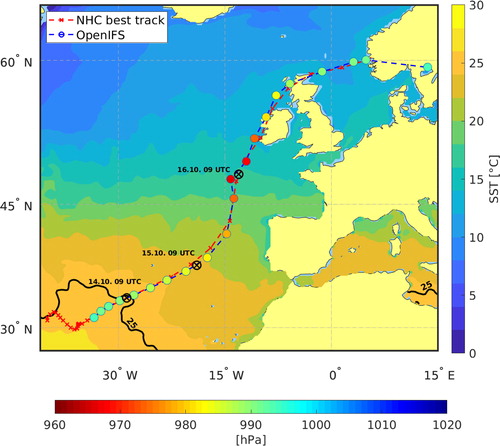
The storm, which was named as Ophelia, was located between two ridges: one to the north over the mid-latitude North Atlantic, and another to the south, over the subtropical Atlantic. Due to this synoptic configuration, the steering currents in the central and eastern North Atlantic were weak. Ophelia stayed almost in the same place during the next few days (note the crosses close to each other in the lower left corner of Fig. 1). Even though the sea surface temperatures beneath Ophelia were only moderately warm (T = 26 °C, see Fig. 1), the relatively cold mid- and upper-troposphere, associated with the positive potential vorticity anomaly resulted in steep lapse rates and vigorous deep convection in the vicinity of the storm’s centre (not shown), which eventually led to the strengthening of Ophelia to a category 1 hurricane on 11 October (Stewart, 2018).

Fig. 1. National Hurricane Center best track for Hurricane Ophelia (red) and OpenIFS track based on minimum sea level pressure (blue). The colours in the OpenIFS track denote minimum sea level pressure in the OpenIFS simulation. The background colours show the sea surface temperatures at 12 UTC 14 October, with 25 °C isotherm contoured. The locations of Ophelia at its peak intensity as a hurricane (9 UTC 14 October), and 24 (9 UTC 15 October) and 48 hours later (9 UTC 16 October) are also indicated.

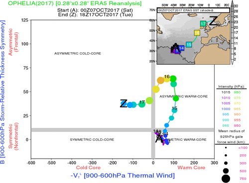
The tropical, transition, and extratropical phases of the storm are estimated using both the phase space diagram of Ophelia (Fig. 2; Hart, 2018) and the NHC report (Stewart, 2018). The phase space diagram is based on ERA5 reanalysis. The storm became asymmetric (B > 10 m) at 12 UTC 14 October, which indicates the onset of the ET. The completion of ET is defined as $-V_T^L$ < 0 m, which in Ophelia’s case took place at 18 UTC 16 October. In the NHC report, however, Ophelia is classified as a hurricane until 18 UTC 15 October, and then as an extratropical storm onwards from 00 UTC 16 October.

Fig. 2. Phase space diagram of Ophelia based on ERA5 reanalysis. The dots are plotted every six hours and the numbers labeled in the dots indicate the days of October 2017. The figure is from Hart (2018) and is used with permission.

The spatial fields of 900–800-hPa relative vorticity and tropopause level (2.0-PVU) potential temperature based on ERA5 reanalysis are depicted in Fig. 3a, d and g. The figures are from three different times with a 24-hour interval: 9 UTC 14 October, 9 UTC 15 October, and 9 UTC 16 October. At the first time (9 UTC 14 October) the storm has just started ET (Fig. 2), but was still classified as a category 3 hurricane based on the NHC report (Stewart, 2018). The second time (9 UTC 15 October) represents the transition phase of the storm, and the latest time (9 UTC 16 October) corresponds with the time of Ophelia’s maximum intensity as an extratropical storm, which falls between the classified extratropical phases of the diagram and the NHC report. Hereafter, these three times represent the tropical, transition, and extratropical phases of the storm. The location of Ophelia at these three times is also marked in Fig. 1 with black crosses.

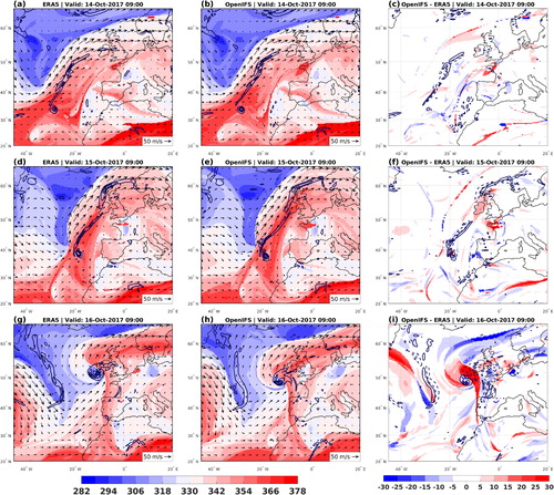
Fig. 3. Potential temperature (colours, K) and wind (arrows, reference arrow in the lower-right corner) on dynamic tropopause (2.0 PVU), and relative vorticity averaged over 950–850-hPa layer (contours, with 2 × 10⁻⁴ s⁻¹ interval starting from 10⁻⁴ s⁻¹) from ERA5 (left column) and OpenIFS (middle column) at 9 UTC 14 October (upper row), 9 UTC 15 October (middle row), and 9 UTC 16 October (bottom row). The difference OpenIFS - ERA5 of potential temperature on 2.0 PVU (colours, with a separate colourbar) and relative vorticity averaged over 950–850-hPa layer (contours) are shown in the right column. In panels (c), (f) and (i), the solid lines show areas where the relative vorticity is higher in OpenIFS than in ERA5, and the dashed lines show the opposite.

From Fig. 3a, Ophelia can be identified as a circular area of low-level vorticity roughly at the location of 35°N and 30°W. To the north and northeast of Ophelia, there is a long vorticity maximum associated with a frontal zone. On 12 October, Ophelia was steered by increased upper-level winds due to a large long-wave trough, which had propagated from North America to the North Atlantic (not shown). Two days later, on 14 October, the trough is visible in Fig. 3a with blue colours (lower potential temperature on the dynamic tropopause). Ophelia is experiencing south-westerly upper-level flow (arrows in Fig. 3a). The trough started to direct Ophelia towards Europe, and at 12 UTC 14 October, regardless of relatively cool sea surface temperatures (T = 25 °C, Fig. 1), Ophelia reached its peak intensity as a category 3 hurricane (roughly at the time of Fig. 3a). The strengthening was possible because of strong deep convection near the storm centre allowed by steep lapse rates due to cooler than average ambient temperatures in the mid- and upper troposphere (Stewart, 2018).

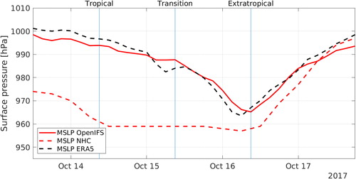
Later, on 15 October, Ophelia started losing its tropical characteristics due to the increased wind shear caused by the jet stream associated with the upper-level trough (Fig. 3d). The low-level vorticity maximum was no longer circular, but slightly stretched meridionally towards the frontal zone (Fig. 3d). Although this behaviour led to a decrease of surface wind speeds (Stewart, 2018), the favorable interaction with the upper-level trough ensured that the minimum surface pressure did not start to increase (Fig. 4, red dashed line). The decrease of maximum wind speeds with steady surface pressure can be explained with the growing horizontal size of the storm. This can be seen from Fig. 2 as growing size of the circles, indicating larger radius of 925-hPa gale-force winds when the storm is approaching the extratropical phase.

Fig. 4. Time series of mean sea level pressure at the cyclone centre based on OpenIFS (solid red line), ERA5 reanalysis (dashed black line), and National Hurricane Center best track data (dashed red line). The vertical lines mark the tropical, transition, and extratropical phases of the cyclone.

The favorable interaction with the upper-level trough is consistent with the results of Hart et al. (2006). They showed that tropical cyclones interacting closely with negatively tilted large-scale troughs are more likely to undergo post-ET intensification than cyclones interacting further apart and with positively tilted troughs. Investigation of ERA5 reanalysis data revealed that the 500-hPa trough preceding Ophelia’s transition was indeed slightly negatively tilted, and the location of Ophelia relative to the trough (not shown) was very similar to fig. 12b in Hart et al. (2006). In addition, the enhanced upper-level divergence caused by the right entrance region of the jet stream (see Fig. 3a and d) most likely enhanced Ophelia’s vertical mass flux during the ET, and, thus, helped Ophelia to remain as an intense storm during the transition phase. The fact that Ophelia remained its intensity is in line with the results of Davis et al (2008) and Leroux et al. (2013), who both showed tropical cyclones intensifying in a presence of vertical wind shear caused by the upper-level trough.

Based on the ERA5 reanalysis, at 9 UTC 15 October the circular area of high vorticity associated with Ophelia had almost merged with the more linear frontal vorticity (Fig. 3d). The presence of both areas of vorticity indicates that the system had both tropical and extratropical characteristics and, thus, Ophelia is undergoing extratropical transition at this time. Based on Stewart (2018), the ET of Ophelia was completed at 00 UTC 16 October, which falls in between the times in Fig. 3d and 3g.

Favourable interaction with the upper-level trough helped Ophelia still deepen slightly as a powerful post-tropical cyclone. NHC analysis suggests a pressure minimum of 957 hPa at 9 UTC 16 October (Fig. 4), when Ophelia was just about to make landfall to Ireland (Fig. 3g). Soon after hitting Ireland, Ophelia started to weaken quite rapidly (Fig. 4). The storm further moved across northern Scotland on 17 October, and finally dissipated over Norway on 18 October (Fig. 1).

4. Comparison of OpenIFS simulation to ERA5 data

Figure 1 shows the track of Ophelia based on minimum sea level pressure in the OpenIFS simulation and the analysed track according to NHC. The agreement between the tracks is very good, and shows only slight difference in the area west and southwest from the British isles. This is the area where Ophelia was located when it underwent ET, a process known to be challenging to simulate correctly by numerical weather prediction models (e.g. Evans et al., 2017).

Figure 3 compares the spatial fields of low-level vorticity and upper-level potential temperature between ERA5 (left column) and OpenIFS (middle column). Their differences (OpenIFS - ERA5) at the three time steps are shown in the right column. The fields are very similar to each other during the tropical phase at 9 UTC 14 October (Fig. 3a–c). This agreement continues the next day, when the storm was in the middle of its transition process (Fig. 3d–f). On 16 October, however, there is a slight timing discrepancy between the ERA5 and OpenIFS fields (Fig. 3g–i). While in ERA5 the storm had already passed 50°N latitude by 9 UTC 16 October (Fig. 3g), in our model simulation the storm propagates slightly slower, and remains south of 50°N at this time (Fig. 3h). For this reason, the amplified downstream ridge is also located somewhat further south in OpenIFS, which can be seen particularly from Fig. 3i as an area of large positive difference in upper-level potential temperatures west from the British isles.

Figure 4 depicts the minimum surface pressure of the storm based on the OpenIFS simulation (red solid line) compared to the analysed minimum surface pressure by NHC (red dashed line) and ERA5 reanalysis (black dashed line). During the tropical phase of the storm, both OpenIFS and ERA5 greatly overestimated the central surface pressure. The difference OpenIFS - NHC exceeds 30 hPa at maximum, but was reduced as the storm transformed to a mid-latitude cyclone. OpenIFS also deepened Ophelia more steadily from 13 Oct to 16 Oct, while the NHC best track data shows a clear deepening period on 13–14 October without substantial changes in intensity during the following two days (Fig. 4). Regardless of the large difference between OpenIFS and NHC, the agreement between OpenIFS and ERA5 is generally very good during the whole life cycle of the storm. The implications of the large underestimation of intensity by OpenIFS are discussed further in Section 6.

5. Vertical motion and vorticity tendency diagnostics

5.1. Comparison between calculated and model-simulated vertical motions and vorticity tendencies

In this subsection, the solution of the omega equation (ω_TOT) and the vorticity equation ($\frac{\partial \zeta }{\partial t_{\mathit{TOT}}}$) are compared to vertical motion and vorticity tendency from the OpenIFS output (ω_OIFS and $\frac{\partial \zeta }{\partial t_{\mathit{OIFS}}},$ respectively). The latter is estimated as a central difference from the one-hour time series of the simulated relative vorticity fields.

Figure 5a and b shows ω_TOT and ω_OIFS at 700 hPa at 21 UTC 15 October. Their difference is depicted in Fig. 5c. The similarity between the fields is striking. There are some small differences, for example, in the area of descent to the west of the storm.

Fig. 5. The solution of the omega equation (ω_TOT) (a), omega directly from OpenIFS output (ω_OIFS) (b), and the difference ω_TOT - ω_OIFS at 700 hPa. The same but for vorticity tendencies at the 900–800-hPa layer is shown in panels (d)–(f). Time is at 21 UTC 15 October 2017. Unit in (a)–(c) is Pa s⁻¹, and in (d)–(f) s⁻². Contours in (a)–(c) show mean sea level pressure with 4-hPa interval, and in (d)–(f) relative vorticity averaged over 900–800 hPa starting from 5 × 10⁻⁵ s⁻¹, with 5 × 10⁻⁵ s⁻¹ interval.

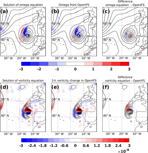
Vorticity and particularly its tendency fields are often very noisy and contain lots of small-scale variation. For this reason, finding a signal related to synoptic-scale weather systems from the vorticity tendency fields can be challenging. To make the interpretation easier, the vorticity tendencies presented in this paper are smoothed by setting the coefficients for total wave numbers more than 127 to zero. This T127 spectral truncation, which corresponds approximately to 165-km grid spacing, was performed after solving the vorticity equation with OZO, using data with full model truncation. The vorticity and its tendency fields in full T639 resolution are attached in the supplementary material of this study. For vertical motion fields, no smoothing is applied because vertical motion fields at T639 resolution are much smoother than the corresponding vorticity tendency fields.

Figure 5d, e and f shows $\frac{\partial \zeta }{\partial t_{\mathit{TOT}}},\frac{\partial \zeta }{\partial t_{\mathit{OIFS}}},$ and their difference at 21 UTC 15 October, respectively. The agreement between the vorticity tendency fields is very good. However, the $\frac{\partial \zeta }{\partial t_{\mathit{OIFS}}}$ field is overall slightly smoother, which comes from the approximation of the time derivative with the central difference method using one-hour time intervals. There is also a moderate positive bias in the centre of the cyclone, which may result from the relatively rough estimation of the imbalance term with one-hour time resolution, which will be discussed further in Section 6.

Spatial correlations between ω_TOT and ω_OIFS, and between $\frac{\partial \zeta }{\partial t_{\mathit{TOT}}}$ and $\frac{\partial \zeta }{\partial t_{\mathit{OIFS}}}$ as a function of pressure are presented in Fig. 6. The correlations have been calculated from a 10° × 10° moving box which followed the centre of Ophelia, and averaged over the time period 15 UTC 13 October - 12 UTC 18 October. In addition, the correlations of vorticity tendencies are given for both T127 and T639 spectral resolutions.

Fig. 6. Correlation between ω_OIFS and the solution of the omega equation (blue), and correlation between $\frac{\partial \zeta }{\partial t_{\mathit{OIFS}}}$ and the solution of the vorticity equation (red) as a function of pressure. The values have been calculated from a 10° × 10° moving box centred to the centre of Ophelia, and averaged over the time period 15 UTC 13 October–12 UTC 18 October.

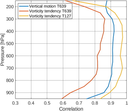
The correlation of vorticity tendencies at T127 resolution clearly exceeds the correlation at T639 resolution. T127 shows correlations of up to 0.97 in the mid-troposphere, while T639 barely exceeds 0.85. The correlation for vertical motions is between those for the vorticity tendencies at the T127 and T639 resolutions. This order of performance reflects the horizontal scale of the fields: the smaller the scale, the worse the correlation. Nevertheless, the key point from Fig. 6 is that the correlations are high, which means that the method of solving the equations is valid.

5.2. Tropical phase

Figure 7 shows the 700-hPa vertical motion induced by the individual forcing components (Fig. 7b–f) and their sum (Fig. 7a) at 9 UTC 14 October, i.e. two days before the maximum intensity of the storm. ω_TOT in Fig. 7a shows strong ascent concentrated on the downshear (eastern) half of the storm, which is mainly caused by diabatic heating (Fig. 7e). This is a typical place for convective cells in tropical cyclones: previous studies have shown that convection usually initiates downshear right and intensifies downshear left of the storm (e.g. Foerster et al., 2014; DeHart et al., 2014).

Fig. 7. Vertical motion (shading, Pa s⁻¹) at 700 hPa at 9 UTC 14 October (tropical phase). The panel (a) shows the total vertical motion due to all five forcing terms [the sum of terms (b)–(f)]. Panels (b)–(f) show the contributions from individual forcing terms: vertical motion due to (b) vorticity advection, (c) thermal advection, (d) friction, (e) diabatic heating, and (f) the imbalance term. The contours show sea level pressure with 4-hPa interval.

In addition to diabatic heating, a minor contribution to vertical motion comes from thermal advection (Fig. 7c), which is due to advection of warm air from the subtropics towards mid-latitudes. In contrast, vorticity advection (Fig. 7b) contributes negligibly to the vertical motion at 700 hPa during the tropical phase of the storm. Similarly, the vertical motion caused by friction is near zero (Fig 7d). Note, however, that the vertical motion due to friction reaches its maximum at levels lower than 700 hPa (Stepanyuk et al., 2017).

Examination of vertical velocity fields from 500 hPa and 300 hPa (not shown) revealed that the pattern does not change substantially with height. In particular, the vertical motion due to diabatic heating (ω_Q) is equally strong higher up in the atmosphere, while vertical motion due to thermal advection (ω_T) shows some signs of weakening with height. Vertical motion due to vorticity advection (ω_V) is still negligible at 500 hPa, but has some weak ascent at 300 hPa, located on the western half of the cyclone centre.

Vorticity tendencies due to the different forcing mechanisms at the same time are presented in Fig. 8. The total vorticity tendency field (Fig. 8a) shows a typical positive-negative dipole, which moves the storm eastward. Almost all of this vorticity tendency is caused by vorticity advection (Fig. 8b). Note also that even though vorticity advection is important for the movement of the cyclone, it does not cause significant vertical motion (Fig. 7b).

Fig. 8. Vorticity tendency (shading, s⁻²) averaged over the 900–800-hPa layer at 9 UTC 14 October (tropical phase). The panel (a) shows the total vorticity tendency due to all five forcing terms [the sum of terms (b)–(f)]. Panels (b)–(f) show the contributions from individual forcing terms: vorticity tendency due to (b) vorticity advection, (c) thermal advection, (d) friction, (e) diabatic heating, and (f) the imbalance term. The contours show relative vorticity, starting from 5 × 10⁻⁵ s⁻¹, with 5 × 10⁻⁵ s⁻¹ interval.

A small part of the vorticity tendency originates also from diabatic heating (Fig. 8e). This field has some positive values at the centre of the storm, which means that the system is intensifying due to diabatic heating. The latent heat release in the convective clouds enhances rising motion, which, in turn, causes low-level convergence to the lower troposphere. The convergence increases vorticity at the cyclone centre via stretching term (RHS term 2 in Eq. 13(13) $${\left(\frac{\partial \zeta }{\partial t}\right)}_X=-{\omega }_X\frac{\partial \zeta }{\partial p}+(\zeta +f)\frac{\partial {\omega }_X}{\partial p}+\mathit{k}·\left(\frac{\partial \mathit{V}}{\partial p}\times \mathbf{\nabla }{\omega }_X\right),X=T,Q,A$$(13) ).

5.3. Transition phase

At 9 UTC 15 October, when Ophelia is in the middle of its transition to a mid-latitude cyclone, baroclinic processes start to be more important for the cyclone development. The sea level pressure field presented in Fig. 9 shows a trough-like feature to the north of the storm, indicating the presence of a frontal zone (see also Fig. 3e). This area also features large-scale ascent induced by vorticity advection (Fig. 9b). The area of ascent north of Ophelia is caused by the upper-level forcing by the approaching mid-latitude trough.

Fig. 9. As Fig. 7, but at 9 UTC 15 October (transition phase).

The vertical motion associated with thermal advection (ω_T, Fig. 9c) has more small-scale structures compared to the vertical motion associated with vorticity advection (ω_V). Consistent with the studies of Räisänen (1995) and R17, ω_V tends to have larger scale but lower magnitude compared to ω_T. The rising motion caused by thermal advection is concentrated on the eastern side of the storm, in the area of warm air advection, while the cold air advection on the western side the storm is causing some sinking motion.

The largest contribution to ω_TOT (Fig. 9a) comes still from diabatic heating (Fig. 9e), with very strong convective ascent on the downshear side of the storm, which is starting to extend north, towards the frontal zone. One notable difference compared to the situation during the tropical phase (Fig. 7a) is the increased compensating sinking motion west of the rising motion, which is caused by diabatic cooling (Fig. 7e). As this descent due to ω_Q coincides partly with the sinking motion caused by the cold air advection (especially 6–9 hours after the time in Fig. 9, not shown), we suspect that the cooling caused by evaporation/melting of cloud droplets is enhancing the sinking motion caused by the cold air advection in this area.

The imbalance term (Fig. 9f) also shows some vertical motion in the vicinity of the storm centre. The areas of descent coincide with areas of ascent in ω_T (Fig. 9c) and vice versa. This tendency of the imbalance term to compensate the effect of thermal advection has been documented earlier in R17, and the physical reason for this compensating effect is explained next. In the real atmosphere, the temperature tendencies caused by thermal advection are often small by their temporal and spatial scales, particularly at low levels. For this reason, the atmosphere usually does not have time to adjust to the new situation and thus compensating vertical motion does not take place. These situations are taken into account by the imbalance term, which often cancels out the effect of thermal advection.

In the transition phase, the low-level vorticity field associated with Ophelia is no longer a symmetric, circular blob, but is extended meridionally towards the frontal zone (Fig. 10, and the full-resolution vorticity in Fig. 3c). This extension of vorticity is mainly caused by diabatic heating, which shows positive vorticity tendency both in the frontal zone and in the vicinity of the storm’s centre (Fig. 10e). Vorticity advection is still mainly contributing to the motion of the storm, as the tendency at the storm’s centre is close to zero. Vorticity tendencies caused by the other processes (thermal advection, friction, and the imbalance term) are very small. Only thermal advection (Fig. 10c) contributes slightly to the eastward movement of the storm by inducing a similar, but much weaker dipole pattern as the vorticity advection.

Fig. 10. As Fig. 8, but at 9 UTC 15 October (transition phase).

5.4. Extratropical phase

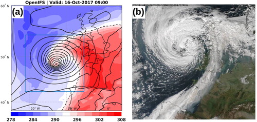
Figure 11a presents the potential temperature at 850 hPa at the extratropical phase of Ophelia (9 UTC 16 October). This is the time when Ophelia reaches its maximum intensity as an extratropical storm (Fig. 4) and when fronts are evident. Based on Fig. 11a, the cold front is approximately perpendicular to the warm front (so called T-bone structure). The warm and cold fronts are however not connected. This gap between the fronts is filled by the warm air mass, which extends all the way to the core of the cyclone, forming a classic warm seclusion. The structure resembles the Shapiro–Keyser conceptual model of extratropical cyclones (Shapiro and Keyser, 1990). Figure 11b shows the satellite image at 1243 UTC 16 October. The bent back warm front and the long cold front are clearly visible.

Fig. 11. Potential temperature at 850 hPa (colours, 294 K isentrope contoured with dashed line) at 9 UTC 16 October (extratropical phase) in the OpenIFS simulation (a), and a visible satellite image captured at 1243 UTC 16 October 2017 (b). Contours in (a) represent mean sea level pressure with 4-hPa intervals, and the blue rectangle in (a) marks the area shown in Figs. 12 and 13. Satellite image copyright NERC Satellite Receiving Station, Dundee University, Scotland (http://www.sat.dundee.ac.uk).

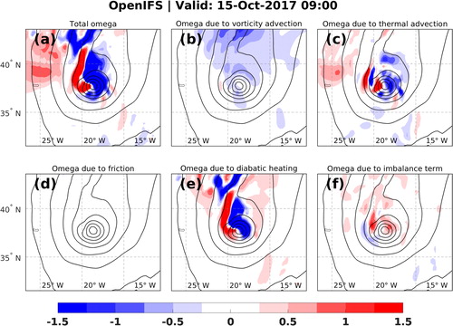
Figure 12 represents the vertical motion induced by the different forcing terms at the same time as Fig. 11a. There is a notable expansion of the wind field of the storm, which can be seen from the larger area of strong pressure gradient compared to the situations 24 hours (Fig. 9) and 48 hours (Fig. 7) earlier. The expansion of wind field is a typical behaviour of cyclones undergoing ET (Evans et al., 2017).

Fig. 12. As Fig. 7, but at 9 UTC 16 October (extratropical phase). The dashed line shows the 294 K isentrope at 850 hPa.

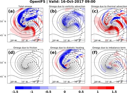
From Fig. 12a it can be seen that the ascent is concentrated on the edges of the warm sector. The ascent on the western edge, namely within the warm front, is dominated by diabatic heating (Fig. 12e). The ascent on the eastern edge of the sector is more due to thermal advection (Fig. 12c). In addition, almost all of the sinking motion within the storm is caused by thermal advection, particularly on the southern side of the centre, due to cold air advection as polar maritime air flows eastward behind the cold front. This area of cold-air advection is also visible in the satellite image as mostly cloud-free (Fig. 11b).

Vorticity advection (Fig. 12b) generates ascent nearly everywhere within the storm, and this ascent is more evenly distributed in the warm sector of the storm than the ascent caused by other forcings. In addition, ω_T tends to compensate ω_V within the warm sector and near the cold front.

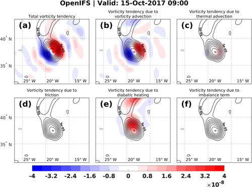
Although the T127 truncation used in the low-level vorticity fields in Fig. 13 hides partly the frontal structures, the vorticity field shows weak vorticity maxima north and east of the storm centre, which are associated with the warm and cold fronts of the system. The vorticity tendency caused by vorticity advection (Fig. 13b) is still close to zero at the storm centre and hence not contributing to the strengthening of the storm. Compared to the situation 24 hours earlier (Fig. 10b), the field shows now more smaller-scale structures. The most notable addition to the positive-negative dipole centred at the storm centre (Fig. 10b) is a similar dipole around the cold front.

Fig. 13. As Fig. 8, but at 9 UTC 16 October (extratropical phase). The dashed line shows the 294 K isentrope at 850 hPa.

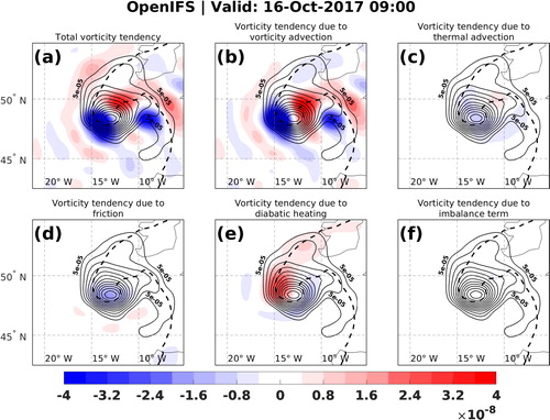
Thermal advection, which only made a very small contribution to Ophelia’s intensity in earlier stages (Figs. 8c and 10c), shows now a negative vorticity tendency on the centre and the southern side of the storm (Fig. 13c). The negative vorticity tendency is due to sinking motion caused by the cold-air advection. Sinking motion leads to divergence in the lower troposphere, which vertically compresses the air column and, thus, decreases the vorticity.

Unlike during the tropical and transition phases, friction is now considerably damping the development of the cyclone by inducing a negative vorticity tendency at the cyclone centre (Fig. 13d). One reason for this behaviour is because the maximum of ω_F (the ascent associated with the Ekman pumping) rises from 950 hPa during the tropical phase to 850 hPa during the extratropical phase (not shown), consistently with the growth of the horizontal scale of the storm. The ascent spreads the effect of the surface friction upwards via the indirect terms (RHS terms 2–4 in Eq. 12(12) $${\left(\frac{\partial \zeta }{\partial t}\right)}_F=\mathit{k}·\mathbf{\nabla }\times \mathit{F}-{\omega }_F\frac{\partial \zeta }{\partial p}+(\zeta +f)\frac{\partial {\omega }_F}{\partial p}+\mathit{k}·\left(\frac{\partial \mathit{V}}{\partial p}\times \mathbf{\nabla }{\omega }_F\right)$$(12) ). For this reason, the vorticity tendency due to friction at 900–800-hPa layer is quite weak in the tropical and transition phases, but increases in the extratropical phase. We also suspect the effect of friction could be slightly underestimated in the tropical phase. This issue is further discussed in Section 6.

The intense vorticity production by diabatic heating within the bent back warm front to the west of the surface low (Fig. 13e) probably contributes to the decay of Ophelia. The reason is that diabatic heating in the mid-troposphere leads to negative vorticity tendency higher up in the atmosphere, to the west of the upper-level trough (not shown). As the generation of vorticity due to diabatic heating slows down the northeastward movement of the surface low (Fig. 13e), the destruction of vorticity does the opposite at the upper levels. As a consequence, the diabatic heating acts to make Ophelia’s trough axis vertically stacked faster which is unfavorable for further intensification, because the area of positive upper-level vorticity advection is not situated above the surface low (not shown). As a result, the vorticity tendency caused by the non-divergent vorticity advection at the centre of low-level cyclone remains very modest on 16 October (Fig. 14d).

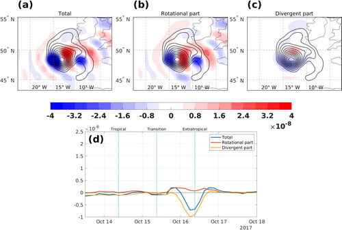
Fig. 14. Vorticity tendency induced by (a) total vorticity advection, (b) vorticity advection by rotational winds, and (c) vorticity advection by divergent winds at 9 UTC 16 October (extratropical phase). In d), time series of vorticity advection by rotational winds (red), divergent winds (yellow), and total winds (blue) averaged over 1.5° circle are shown. The times of tropical, transition, and extratropical phases have been marked with vertical lines in (d).

5.5. Vorticity tendencies at the cyclone centre

Figure 15a shows the time evolution of the low-level vorticity tendencies caused by the various forcing terms, averaged within 1.5° radius from the cyclone centre, as identified from the low-level vorticity maximum. The values have been smoothed by a 12-hour moving average, and are, thus, not exactly comparable with vorticity tendencies at the cyclone centre in Figs. 8, 10 and 13. The reason for the 12-hour smoothing is the fact that the amplitudes of the vorticity tendencies are very sensitive to the location of the circle from which the tendencies have been calculated. The sensitivity is especially true for terms which feature a strong positive-negative vorticity tendency dipole, such as the vorticity advection term. In moving systems, the circle is located just in the middle of the dipole, so a small displacement of the circle drastically affects the tendency averaged over the circular area. For this reason, the raw time series has some small time-scale variation which we wanted to eliminate with the moving averaging.

Fig. 15. Time series of vorticity tendencies caused by (a) different forcing terms and (b) different diabatic heating components. The values have been averaged over the 900–800-hPa layer and over a circular area with a 1.5° radius centred on the maximum of the T127 vorticity field. All values are 12-hour moving averages. The times of tropical, transition, and extratropical phases have been marked with vertical lines.

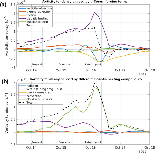
In general, diabatic heating (Fig. 15a, purple line) dominates the generation of cyclonic vorticity during the whole life cycle of Ophelia. The contribution of diabatic heating increases towards the transition period, and peaks just before the deepest stage of the storm, at 3 UTC 16 October. We suspect that the major part of the vorticity increase due to diabatic heating comes from the stretching term (RHS term 2 in Eq. 13(13) $${\left(\frac{\partial \zeta }{\partial t}\right)}_X=-{\omega }_X\frac{\partial \zeta }{\partial p}+(\zeta +f)\frac{\partial {\omega }_X}{\partial p}+\mathit{k}·\left(\frac{\partial \mathit{V}}{\partial p}\times \mathbf{\nabla }{\omega }_X\right),X=T,Q,A$$(13) ). The contributions of different model parametrization schemes to the diabatic heating and the associated vorticity tendencies are studied in more detail in subsection 5.7.

Vorticity advection (Fig. 15a, blue line) is often considered a very important forcing for the development of mid-latitude cyclones, but is found to have neutral or even negative influence for the evolution of Ophelia at 900–800 hPa, varying around zero with the largest negative vorticity tendency right at the deepest stage of the storm. As discussed in the next subsection, the large negative vorticity tendency at the deepest stage is associated with the divergent-wind contribution to vorticity advection.

Thermal advection (Fig. 15a, red line) has the second largest effect on the development of Ophelia during its tropical phase. For the atmosphere, the effect of warm air advection is similar to the effect of diabatic heating; both induce mid-tropospheric rising motion, and hence by mass continuity horizontal convergence in the lower troposphere, which acts to increase cyclonic vorticity. After the transition, the cold-air advection behind the cold front has the opposite influence on the cyclone.

The vorticity tendency caused by friction (Fig. 15a, yellow line) is continuously negative, and its effect grows when Ophelia reaches the extratropical phase. As explained in the earlier subsection, this is mostly due to the increase of ω_F in the extratropical phase.

5.6. Effect of vorticity advection by divergent and rotational winds

As shown in Fig 15a, vorticity advection causes a predominantly negative vorticity tendency near the cyclone centre during the life cycle of Ophelia. This negative vorticity tendency peaks at 3 UTC 16 October, at the moment when the total vorticity tendency is at its highest (Fig. 15a, dashed line). To understand this behaviour, the vorticity tendencies caused by ${\mathit{V}}_{\psi }$ and ${\mathit{V}}_{\chi }$ together with their sum are presented in Fig. 14a–c. Figure 14d shows the corresponding time series at the cyclone centre.

When looking at the spatial fields, there is notable similarity between the vorticity tendency by total vorticity advection (Fig. 14a, same as Fig. 13b) and the vorticity tendency due to rotational wind vorticity advection (Fig. 14b). Thus, the major part of the total vorticity advection is caused by the rotational wind.

However, the crucial issue for the cyclone intensity are the vorticity tendencies at the vicinity of the cyclone centre (Fig. 14d). It can be clearly seen that the increase in negative vorticity tendency due to total vorticity advection on 16 October is solely due to vorticity advection by ${\mathit{V}}_{\chi }.$ Instead, vorticity advection by ${\mathit{V}}_{\psi }$ induces weak, but mainly positive vorticity tendency during the transition period. The negative vorticity tendency due to vorticity advection by ${\mathit{V}}_{\chi }$ can be seen also from Fig. 14c, where the negative values are spread over the cyclone centre.

The physical reason for the negative vorticity tendency caused by ${\mathit{V}}_{\chi }$ at the transition time is the secondary circulation of the cyclone. When the hurricane transforms into a mid-latitude cyclone, its wind field expands and the convergent flow towards the cyclone centre near the surface increases, in part due to friction but also due to other processes that cause lower-tropospheric vertical motion above the cyclone centre. The divergent component of the wind transports air with lower cyclonic vorticity into the area of high cyclonic vorticity. This negative vorticity advection produces negative vorticity tendency, which peaks when the cyclone intensity and its secondary circulation is at its highest. These results align well with R17 and Räisänen (1997).

The divergent flow causing the anticyclonic vorticity advection is due to all processes which causes convergence towards the centre of the storm, including diabatic heating. However, note that the vorticity tendency caused by ${\mathit{V}}_{\chi }$ accounts also for the stretching due to vorticity advection (RHS term 3 in Eq. 11(11) $${\left(\frac{\partial \zeta }{\partial t}\right)}_V=-\mathit{V}\cdot \mathbf{\nabla }(\zeta +f)-{\omega }_V\frac{\partial \zeta }{\partial p}+(\zeta +f)\frac{\partial {\omega }_V}{\partial p}+\mathit{k}·\left(\frac{\partial \mathit{V}}{\partial p}\times \mathbf{\nabla }{\omega }_V\right)$$(11) ). Nevertheless, we suspect that the stretching due to vorticity advection is actually quite modest during the tropical and transition phases of the storm, because of the weak ω_V at the cyclone centre (Figs. 7b and 9b).

5.7. The contributions from different model parametrizations to diabatic heating

Diabatic processes were the dominant forcing in the ET of Ophelia (Fig. 15a). But which diabatic processes were the most important?

In OpenIFS, the total temperature tendency by diabatic heating consists of five parts (Eq. 15(15) $$Q=Q_r+Q_d+Q_g+Q_c+Q_{mp}$$(15) and Table 2). Figure 15b shows the contributions of these five components to the vorticity tendency in the centre of the storm. The vorticity tendencies induced by radiation (blue), vertical diffusion + orographic drag + surface processes (red), and gravity wave drag (yellow) are negligible within 1.5° radius of the storm centre and also elsewhere in the vicinity of the storm (not shown). The vorticity tendencies due to convection (purple) and cloud microphysics (green) were much more important.

The vorticity tendency caused by convection (purple) is the dominant forcing in the beginning of the simulation, during the hurricane phase of Ophelia. From 15 October onwards, the cloud microphysics scheme (green) becomes more important. Finally, in the extratropical phase (at 9 UTC 16 October), the convection scheme does not anymore enhance the cyclone development. At this point, the heating generated by the cloud microphysics scheme is the only diabatic process that produces positive vorticity within 1.5° radius of the cyclone centre.

More information on the different sources of model-simulated diabatic heating can be obtained from the maps. Figure 16 shows the vertical motion induced by the convection scheme (Fig. 16a) and the cloud microphysics scheme (Fig. 16b) at the tropical phase of the storm (9 UTC 14 October). The convection scheme produces ascent which extends horizontally over a large area around the storm, whereas the vertical motions generated by the cloud microphysics scheme are more localized, mainly near the cyclone centre. Figure 16e and f represents the same situation but for the vorticity tendencies. The convection scheme (Fig. 16e) produces cyclonic vorticity in the area of ascent, in the south-east quadrant of the storm. The cloud microphysics scheme (Fig. 16f) generates negligible vorticity tendency, in agreement with Fig. 15b.

Fig. 16. Panels (a) – (d) show vertical motion (shading, Pa s⁻¹) at 700 hPa and sea level pressure (contours, with 4-hPa interval), and panels (e) – (h) show vorticity tendency (shading, s⁻²) and relative vorticity (contours, starting from 5 × 10⁻⁵ s⁻¹, with 5 × 10⁻⁵ s⁻¹ interval) averaged over the 900–800-hPa layer. The left-hand panels [(a), (c), (e), and (g)] show vertical motion and vorticity tendency due to the convection parametrization, and the right-hand panels [(b), (d), (f) and (h)] show vertical motion and vorticity tendency due to the microphysics parametrization. The upper panels in both vertical motion [(a) and (b)] and in vorticity tendency [(e) and (f)] show the situation at 9 UTC 14 October (tropical phase), and the lower panels [(c), (d), (g) and (h)] at 9 UTC 16 October (extratropical phase). The size of the panels is 16° longitude by 12° latitude, centred on the cyclone vorticity maximum.

Vertical motions and vorticity tendencies due to convection and cloud microphysics schemes at the extratropical phase of the storm (9 UTC 16 October) are presented in Fig. 16c, d, g and h. The convection scheme produces ascent in localised spots within the warm sector and cold front of the storm (Fig. 16c). In particular, there is strong convective lifting occurring over southern Ireland. However, the large-scale rising motion in the warm front is enhanced by the diabatic heating generated by the cloud microphysics scheme (Fig. 16d). Furthermore, there are areas of cancellation between these two schemes. One example is along the part of the cold front closest to the cyclone centre, to the northeast of the storm, where the compensating sinking motion from the cloud microphysics scheme coincides with rising motion associated with the convection scheme. We suspect that convection produces heating via condensation and freezing of water, but part of the rain is evaporated before reaching the surface. Although the convective parametrization produces ascent within the warm sector of the storm, the vorticity tendency caused by it is very weak (Fig. 16g). Instead, the cloud microphysics parametrization generates notably more cyclonic vorticity (Fig. 16h), which is co-located with the frontal ascent.

This analysis illustrates how the emphasis of diabatic heating, and more specifically the latent heat release from the condensation/freezing of water vapour, changes from the convective parametrization to the cloud microphysics parametrization during the ET of the storm. This change in the importance of parametrization schemes is particularly notable in vorticity tendencies near the cyclone centre (Fig. 15b), which effectively affect the strength of the storm. The reason for this change is firstly the shift of convective ascent further away from the storm centre to the area of the warm sector, and secondly the formation of the warm front in which the cloud microphysics scheme in the model is activated.

The diabatic heating components used in this analysis (Table 2) are naturally OpenIFS-specific. In other numerical models, the partitioning of Q into contributions from different heating processes may be done differently. Nevertheless, we would still expect that the shift from convective heating towards latent heat release associated with larger-scale ascent (which is represented by the cloud microphysics scheme) is a typical characteristic of the ET process.

6. Discussion

Although the re-intensification of Hurricane Ophelia when it struck Ireland as a post-tropical storm occurred during favorable interaction with an upper-level trough, we found the direct effect of the adiabatic upper-level forcing on the lower tropospheric storm to be relatively modest. Rather, our results suggest that the effect of the upper-level forcing was strongly amplified by diabatic processes. This outcome emphasizes the importance of resolving diabatic processes correctly in climate models. Since the effect of diabatic heating on the intensity of extratropical cyclones is quite sensitive to the model resolution (Willison et al., 2013), high-resolution simulations are required to investigate the future projections of post-tropical storms. Fortunately, this is already the case in some recent studies (e.g. Haarsma et al., 2013; Baatsen et al., 2015).

OpenIFS underestimated the intensity of Ophelia during its tropical phase, seen as higher minimum sea level pressure in OpenIFS than in the NHC analysis (Fig. 4). Yamaguchi et al. (2017) reported that all the major global numerical weather prediction models tend to underestimate tropical cyclone intensity, especially when the minimum sea level pressure is 940 hPa or below. They found this systematic error to be present even at the initialization time of the forecasts, which implies that the resolution of the models may be the biggest culprit for the error. Hodges and Klingaman (2019) reported approximately 8 hPa intensity error of tropical cyclones in the Western North Pacific at the initial time of the IFS model forecasts. As our model resolution was coarser than what is typically used in operational weather prediction models, we suspect that the overestimation of sea level pressure (Fig. 4) was primarily due to the coarse resolution. Examination of initial states from the forecast used in this study, and a forecast initialized 24 hours later (at 12 UTC 14 October) revealed that the large overestimation of Ophelia’s minimum surface pressure was present already in the initial conditions. Furthermore, the operational analyses by Climate Forecast System Version 2 (CFSv2), Global Forecast System (GFS) and the Japanese 55-year Reanalysis (JRA-55) also underestimated the minimum pressure of Ophelia approximately 30 hPa during the tropical phase (not shown). The fact that the underestimation of intensity was clearly reduced when the ET was completed and the horizontal scale of the storm was increased, supports our conclusion about low resolution of OpenIFS to capture the small-scale pressure minimum during the tropical phase.

As the intensity of the storm during the tropical phase was clearly underestimated, one can also question the reliability of the magnitude of vorticity tendencies calculated in the centre of the storm during the tropical phase (Fig. 15). This is a relevant aspect which needs to be taken into account when interpreting the results. Firstly, the scale of the storm relative to the size of the moving circle from which the vorticity tendencies (1.5° radius) were calculated is smaller in the tropical phase than in the extratropical phase. This means that the averaging smooths the tendencies more when the storm is small relative to the area of the circle, and this has probably had some effect on the smallness of the vorticity tendency terms in the beginning of our simulation in Fig. 15. Secondly, the model resolution also smooths the local vorticity and its tendency structures close to the eye of the hurricane. For these two reasons, the magnitude of vorticity tendencies during the tropical phase are probably underestimated. A simple solution for this would be to run OpenIFS with higher resolution. However, our diagnostic software has some limitations regarding to the high-resolution runs: the imbalance term grows larger and thus the interpretation of the results becomes increasingly problematic. This issue has been explained in detail in Section 8 of R17. Nevertheless, as the main aim of this study was to focus on the transition and extratropical phases of the storm, we acknowledge the weakness of our results in the tropical phase and leave it for a topic of a possible follow-up study.

In our technical framework, we divided only the atmospheric vertical motion and vorticity tendency into contributions from different forcing terms. For consistency, the division of divergent wind into the same contributions could provide new interesting information on the physical processes affecting the secondary circulation of Ophelia. However, as far as we see, the realization of this decomposition is technically complicated, and would lead in an iterative solution that would significantly complicate the solution of the omega equation. For this reason, the implementation of this functionality is not included to the current version of OZO, but it is something which could be worth of carrying out in the future.

Regarding the performance of OZO, the correlations for vertical motion (Fig. 6) are somewhat worse than in the idealized case in R17. The largest source of numerical errors is the calculation of time derivatives of vorticity and temperature in Eq. 7(7) $$F_A=f\frac{\partial }{\partial p}\left(\frac{\partial \zeta }{\partial t}\right)+\frac{R}{p}{\nabla }^2\left(\frac{\partial T}{\partial t}\right).$$(7) . Because these time derivatives cannot be output directly from OpenIFS, they are approximated with the central difference method with one-hour time interval. By decreasing the time interval, particularly the accuracy of the imbalance term could be improved, which would decrease the difference between ω_TOT and ω_OIFS as shown in Fig. 2 in R17. This would however affect only the magnitude of the imbalance term, which plays a rather small role for the development of Ophelia.

The diabatic heating rate Q and friction F are not available from OpenIFS as instantaneous values, but rather need to be calculated from time-accumulated tendencies over each output interval. Here, we used a one-hour output interval and evaluated these terms as time-averages over a two-hour time span. This averaging had to be done because otherwise the tendencies would have contained information only from the past one hour and, therefore, have featured a 30-minute phase shift compared to other variables. For this reason, a decrease of the output time interval could slightly increase the accuracy of the diabatic heating and friction terms. We do not expect this to affect significantly the main results of this study, as the magnitude of the diabatic heating and friction terms would rather increase than decrease when using a smaller time interval for the averaging.

Our main conclusion is that the diabatic heating was the dominant forcing for the intensity of the low-level cyclone. In the extratropical phase, the diabatic heating came mainly from the microphysics scheme, but we did not have information about the contributions of individual microphysical processes (such as condensation, evaporation, freezing) to the heating. The reason for this is that currently OpenIFS does not have a functionality to output the temperature tendencies associated with these various microphysical processes.

In many previous studies the effect of vorticity advection for the development of post-tropical storms has been estimated using the mid- or upper-level winds (e.g. Klein et al., 2002; Ritchie and Elsberry, 2007) or geostrophic winds (e.g. Milrad et al., 2009; Azad and Sorteberg, 2009). As we calculated the forcing terms at the lower troposphere and accounted also for the divergent circulation and the indirect contributions from vertical motion, our results are naturally not comparable with those listed. DiMego and Bosart (1982), who studied the transformation of Tropical Storm Agnes into an extratropical cyclone, stated that” Differential advection by the divergent part of the wind, although generally weaker, act as a sink of vorticity.” This statement is consistent with our results. Azad and Sorteberg (2014) used a very similar method for the examination of vorticity tendency budgets in regular North Atlantic winter extratropical cyclones. They reported vorticity advection being the most influential low-level forcing for the composite cyclone. Our results with Ophelia do not agree with this, but on the other hand we studied a post-tropical storm, which is somewhat different by its dynamics than the pure extratropical cyclones used in the study by Azad and Sorteberg (2014).

As a final note, this analysis was purposely performed only for the surface cyclone, since we wanted to study the forcing mechanisms responsible for the surface impacts. This was the main motivation why the vorticity tendencies were calculated for the 900–800-hPa layer, and the choice of 700 hPa for the vertical motion analysis. Hence, the main outcome of our study - the importance of diabatic heating for the strength of the surface cyclone - does not apply at higher levels. In fact, the examination of vorticity tendencies at 500 and 250 hPa levels revealed thermal advection being the main contributor to the strength of the upper trough (not shown).

7. Conclusions

This study investigated the extratropical transition of Hurricane Ophelia with the generalized omega equation and vorticity equation. The main aim was to determine the contributions of different adiabatic and diabatic forcing terms for the life cycle of the storm, and identify which of them led to the strengthening of the storm into a powerful post-tropical cyclone when it made landfall in Ireland in October 2017. Our initial hypothesis was that diabatic processes would be dominant in the tropical phase of the cyclone, but baroclinic processes (vorticity advection and thermal advection) would become more important for the cyclone development after its extratropical transition.

The first part of our hypothesis was correct: diabatic heating, and more specifically the release of latent heat, was indeed the dominant forcing during Ophelia’s tropical phase. Latent heat release, ascending motion, and positive low-level vorticity tendency were first produced via the convection scheme, but smoothly changed to the cloud microphysics scheme later, during the transition and the extratropical phases of the storm. Other diabatic heating processes were found to be negligible for the cyclone evolution.

Unlike what we hypothesized, the low-level relative vorticity at the storm centre during the extratropical phase was largely produced by diabatic heating rather than adiabatic processes (vorticity advection or thermal advection). In fact, the net-effect of vorticity advection was actually detrimental for the surface cyclone because the divergent winds within the secondary circulation of the cyclone transported air with less cyclonic vorticity to the centre of the storm, thus reducing the vorticity maximum at the centre. Vorticity advection by the rotational winds did contribute to the intensification of the storm in its extratropical phase, but its contribution was much smaller than that of diabatic heating. Thermal advection, which made a moderate contribution during the tropical phase due to warm-air advection from the subtropics, no longer enhanced the development of the storm during its extratropical phase. The reason for this was the occlusion process, which led cold air advection to wrap from the southwest around the storm and, consequently, to a negative vorticity tendency at the vicinity of the storm centre. The effect of friction was found to increase soon after the extratropical transition, presumably due to the expansion of the wind field. Together with the lack of baroclinic forcings, the effect of friction led to the weakening of the storm after the landfall.

Our results are valid for the surface cyclone, and, thus, not applicable at higher levels. However, it is important to note that diabatic heating, which is largely dominated by the latent heat release in the clouds, requires usually existing rising motion to occur. Thus, although our analysis suggests a very modest direct role for the upper-level forcing, it may still have been important in triggering the large-scale rising motion that generated the latent heat release above the low-level vortex. Based on one case study it is not possible to conclude whether our outcome is typical in post-tropical storms. Therefore, it would be interesting to conduct a statistical study of cyclones undergoing extratropical transition and investigate what is the average role of different adiabatic and diabatic forcing terms for the evolution of post-tropical storms.

Acknowledgements

The authors wish to acknowledge CSC–IT Center for Science, Finland, for computational resources. ECMWF is acknowledged for making the OpenIFS model available and for generating the ERA5 reanalysis. Copernicus Climate Change Service (C3S) is acknowledged for providing access to the ERA5 data. We thank Kevin Hodges for providing the TRACK code and for his advice with the algorithm. Robert Hart is acknowledged for the cyclone phase space diagram, and NERC Satellite Receiving Station, Dundee University, Scotland for the satellite image. Finally, we would like to also thank the three anonymous reviewers for their constructive feedback.

Disclosure statement

No potential conflict of interest was reported by the authors.

Additional information

Funding

MR acknowledges the Doctoral Programme in Atmospheric Sciences (ATM-DP, University of Helsinki) for financial support. VAS is funded by the Academy of Finland Center of Excellence programme (project no. 307331).

References

- Azad, R. and Sorteberg, A. 2009. A diagnosis of warm-core and cold-core extratropical cyclone development using the Zwack–Okossi equation. Atmos. Sci. Lett. 10, 220–225.
- Azad, R. and Sorteberg, A. 2014. The vorticity budgets of North Atlantic winter extratropical cyclone life cycles in MERRA reanalysis. Part I: development phase. J. Atmos. Sci. 71, 3109–3128. doi:10.1175/JAS-D-13-0267.1
- Baatsen, M., Haarsma, R. J., Van Delden, A. J. and De Vries, H. 2015. Severe autumn storms in future western Europe with a warmer Atlantic ocean. Clim. Dyn. 45, 949–964. doi:10.1007/s00382-014-2329-8
- Bentley, A. M., Bosart, L. F. and Keyser, D. 2019. A climatology of extratropical cyclones leading to extreme weather events over central and eastern North America. Mon. Wea. Rev. 147, 1471–1490. doi:10.1175/MWR-D-18-0453.1
- Bieli, M., Camargo, S. J., Sobel, A. H., Evans, J. L. and Hall, T. 2019. A global climatology of extratropical transition part I: characteristics across basins. J. Climate. 32, 3557–3582. doi:10.1175/JCLI-D-17-0518.1
- Browning, K., Panagi, P. and Vaughan, G. 1998. Analysis of an ex-tropical cyclone after its reintensification as a warm-core extratropical cyclone. Q. J. R. Meteorol. Soc. 124, 2329–2356. doi:10.1002/qj.49712455108
- Davis, C. A., Jones, S. C. and Riemer, M. 2008. Hurricane vortex dynamics during Atlantic extratropical transition. J. Atmos. Sci. 65, 714–736. doi:10.1175/2007JAS2488.1
- DeHart, J. C., Houze, R. A. Jr. and Rogers, R. F. 2014. Quadrant distribution of tropical cyclone inner-core kinematics in relation to environmental shear. J. Atmos. Sci. 71, 2713–2732. doi:10.1175/JAS-D-13-0298.1
- DiMego, G. J. and Bosart, L. F. 1982. The transformation of Tropical Storm Agnes into an extratropical cyclone. Part II: moisture, vorticity and kinetic energy budgets. Mon. Wea. Rev. 110, 412–433. doi:10.1175/1520-0493(1982)110<0412:TTOTSA>2.0.CO;2
- Evans, C., Wood, K. M., Aberson, S. D., Archambault, H. M., Milrad, S. M. and co-authors. 2017. The extratropical transition of tropical cyclones. Part I: cyclone evolution and direct impacts. Mon. Wea. Rev. 145, 4317–4344. doi:10.1175/MWR-D-17-0027.1
- Evans, J. L. and Hart, R. E. 2003. Objective indicators of the life cycle evolution of extratropical transition for Atlantic tropical cyclones. Mon. Wea. Rev. 131, 909–925. doi:10.1175/1520-0493(2003)131<0909:OIOTLC>2.0.CO;2
- Feser, F., Schubert-Frisius, M., von Storch, H., Zahn, M., Barcikowska, M. and co-authors. 2015. Hurricane Gonzalo and its extratropical transition to a strong European storm. Bull. Amer. Meteor. Soc. 96, S51–S55. doi:10.1175/BAMS-D-15-00122.1
- Foerster, A. M., Bell, M. M., Harr, P. A. and Jones, S. C. 2014. Observations of the eyewall structure of Typhoon Sinlaku (2008) during the transformation stage of extratropical transition. Mon. Wea. Rev. 142, 3372–3392. doi:10.1175/MWR-D-13-00313.1
- Grams, C. M. and Blumer, S. R. 2015. European high-impact weather caused by the downstream response to the extratropical transition of North Atlantic Hurricane Katia (2011). Geophys. Res. Lett. 42, 8738–8748. doi:10.1002/2015GL066253
- Grams, C. M., Jones, S. C., Davis, C. A., Harr, P. A. and Weissmann, M. 2013. The impact of Typhoon Jangmi (2008) on the midlatitude flow. Part I: upper-level ridgebuilding and modification of the jet. Q. J. R. Meteorol. Soc. 139, 2148–2164. doi:10.1002/qj.2091
- Haarsma, R. J., Hazeleger, W., Severijns, C., De Vries, H., Sterl, A. and co-authors. 2013. More hurricanes to hit western Europe due to global warming. Geophys. Res. Lett. 40, 1783–1788. doi:10.1002/grl.50360
- Hart, R. 2018. Cyclone phase evolution: analyses & forecasts. Online at: http://moe.met.fsu.edu/cyclonephase/archive/2017/gifs/ophelia2017 [accessed 20 May 2019]
- Hart, R. E. 2003. A cyclone phase space derived from thermal wind and thermal asymmetry. Mon. Wea. Rev. 131, 585–616. doi:10.1175/1520-0493(2003)131<0585:ACPSDF>2.0.CO;2
- Hart, R. E. and Evans, J. L. 2001. A climatology of the extratropical transition of Atlantic tropical cyclones. J. Climate 14, 546–564. doi:10.1175/1520-0442(2001)014<0546:ACOTET>2.0.CO;2
- Hart, R. E., Evans, J. L. and Evans, C. 2006. Synoptic composites of the extratropical transition life cycle of North Atlantic tropical cyclones: factors determining posttransition evolution. Mon. Wea. Rev. 134, 553–578. doi:10.1175/MWR3082.1
- Hawcroft, M., Walsh, E., Hodges, K. and Zappa, G. 2018. Significantly increased extreme precipitation expected in Europe and North America from extratropical cyclones. Environ. Res. Lett. 13, 124006. doi:10.1088/1748-9326/aaed59
- Hodges, K. 1995. Feature tracking on the unit sphere. Mon. Wea. Rev. 123, 3458–3465. doi:10.1175/1520-0493(1995)123<3458:FTOTUS>2.0.CO;2
- Hodges, K. and Klingaman, N. 2019. Prediction errors of tropical cyclones in the Western North Pacific in the met office global forecast model. Wea. Forecasting 34, 1189–1209. doi:10.1175/WAF-D-19-0005.1
- Hodges, K. I. 1994. A general method for tracking analysis and its application to meteorological data. Mon. Wea. Rev. 122, 2573–2586. doi:10.1175/1520-0493(1994)122<2573:AGMFTA>2.0.CO;2
- Keller, J. H., Grams, C. M., Riemer, M., Archambault, H. M., Bosart, L. and co-authors. 2018. The Extratropical Transition of Tropical Cyclones Part II: interaction with the midlatitude flow, downstream impacts, and implications for predictability. Mon. Wea. Rev. 147, 1077–1106. doi:10.1175/MWR-D-17-0329.1
- Klein, P. M., Harr, P. A. and Elsberry, R. L. 2002. Extratropical transition of western North Pacific tropical cyclones: midlatitude and tropical cyclone contributions to reintensification. Mon. Wea. Rev. 130, 2240–2259. doi:10.1175/1520-0493(2002)130<2240:ETOWNP>2.0.CO;2
- Leroux, M.-D., Plu, M., Barbary, D., Roux, F. and Arbogast, P. 2013. Dynamical and physical processes leading to tropical cyclone intensification under upper-level trough forcing. J. Atmos. Sci. 70, 2547–2565. doi:10.1175/JAS-D-12-0293.1
- Liu, M., Vecchi, G. A., Smith, J. A. and Murakami, H. 2017. The present-day simulation and twenty-first-century projection of the climatology of extratropical transition in the North Atlantic. J. Climate 30, 2739–2756. doi:10.1175/JCLI-D-16-0352.1
- Milrad, S. M., Atallah, E. H. and Gyakum, J. R. 2009. Dynamical and precipitation structures of poleward-moving tropical cyclones in eastern Canada, 1979–2005. Mon. Wea. Rev. 137, 836–851. doi:10.1175/2008MWR2578.1
- Palmén, E. 1958. Vertical circulation and release of kinetic energy during the development of Hurricane Hazel into an extratropical storm. Tellus 10, 1–23.
- Räisänen, J. 1995. Factors affecting synoptic-scale vertical motions: a statistical study using a generalized omega equation. Mon. Wea. Rev. 123, 2447–2460. doi:10.1175/1520-0493(1995)123<2447:FASSVM>2.0.CO;2
- Räisänen, J. 1997. Height tendency diagnostics using a generalized omega equation, the vorticity equation, and a nonlinear balance equation. Mon. Wea. Rev. 125, 1577–1597. doi:10.1175/1520-0493(1997)125<1577:HTDUAG>2.0.CO;2
- Rantanen, M., Räisänen, J., Lento, J., Stepanyuk, O., Räty, O. and co-authors. 2017. OZO v. 1.0: software for solving a generalised omega equation and the Zwack–Okossi height tendency equation using WRF model output. Geosci. Model Dev. 10, 827–841. doi:10.5194/gmd-10-827-2017
- Reynolds, R. W., Smith, T. M., Liu, C., Chelton, D. B., Casey, K. S. and co-authors. 2007. Daily high-resolution-blended analyses for sea surface temperature. J. Climate 20, 5473–5496. doi:10.1175/2007JCLI1824.1
- Ritchie, E. A. and Elsberry, R. L. 2007. Simulations of the extratropical transition of tropical cyclones: phasing between the upper-level trough and tropical cyclones. Mon. Wea. Rev. 135, 862–876. doi:10.1175/MWR3303.1
- Rolfson, D. M. and Smith, P. J. 1996. A composite diagnosis of synoptic-scale extratropical cyclone development over the United States. Mon. Wea. Rev. 124, 1084–1099. doi:10.1175/1520-0493(1996)124<1084:ACDOSS>2.0.CO;2
- Seiler, C. 2019. A Climatological Assessment of Intense Extratropical Cyclones from the Potential Vorticity Perspective. J. Climate 32, 2369–2380. doi:10.1175/JCLI-D-18-0461.1
- Sekioka, M. 1956. A hypothesis on complex of tropical and extratropical cyclones for typhoon in the middle latitudes. J. Meteorol. Soc. 34, 276–287. doi:10.2151/jmsj1923.34.5_276
- Shapiro, M. A. and Keyser, D. 1990. Fronts, jet streams and the tropopause, in: Extratropical Cyclones. Springer, New York, pp. 167–191.
- Sinclair, V. A. and Dacre, H. F. 2019. Which extra-tropical cyclones contribute most to the transport of moisture in the Southern Hemisphere? J. Geophys. Res. Atmos. 124, 2525–2545. doi:10.1029/2018JD028766
- Stepanyuk, O., Räisänen, J., Sinclair, V. A. and Järvinen, H. 2017. Factors affecting atmospheric vertical motions as analyzed with a generalized omega equation and the OpenIFS model. Tellus A: Dynamic Meteorology and Oceanography 69, 1271563. doi:10.1080/16000870.2016.1271563
- Stewart, S. R. 2018. Tropical Cyclone Report: Hurricane Ophelia, 9–15 October 2017, National Hurricane Center.
- Thorncroft, C. and Jones, S. C. 2000. The extratropical transitions of Hurricanes Felix and Iris in 1995. Mon. Wea. Rev. 128, 947–972. doi:10.1175/1520-0493(2000)128<0947:TETOHF>2.0.CO;2
- Willison, J., Robinson, W. A. and Lackmann, G. M. 2013. The importance of resolving mesoscale latent heating in the North Atlantic storm track. J. Atmos. Sci. 70, 2234–2250. doi:10.1175/JAS-D-12-0226.1
- Yamaguchi, M., Ishida, J., Sato, H. and Nakagawa, M. 2017. WGNE intercomparison of tropical cyclone forecasts by operational NWP models: a quarter century and beyond. Bull. Amer. Meteor. Soc. 98, 2337–2349. doi:10.1175/BAMS-D-16-0133.1
- Zappa, G., Shaffrey, L. C. and Hodges, K. I. 2013. The ability of CMIP5 models to simulate North Atlantic extratropical cyclones. J. Climate 26, 5379–5396. doi:10.1175/JCLI-D-12-00501.1