The impact of climate indices on precipitation variability in Baluchistan, Pakistan

Abstract

Pakistan’s biggest province in terms of area, Baluchistan appears to have been affected from the climate variability since last few decades. No substantive research works have been carried out in analyzing the precipitation variability in Baluchistan and linkage to large-scale teleconnection. The goal of this paper is to determine possible linkages of precipitation with large scale atmospheric and oceanic circulation indices in the months which have shown changes in precipitation trends in Baluchistan. These climate indices may be the possible predictors for the precipitation in Baluchistan in the respective months. Mann-Kendall (MK) statistical test was used to identify the monthly significant precipitation trends in thirteen meteorological stations located in four regions of Baluchistan. The noteworthy trend out of significant trends is selected using Theil and Sen’s slope (TS). Decreasing trend is identified in January whereas increasing trend is identified in June mostly in stations located in North Eastern region of Baluchistan (Region1). The changes in the significant trend in January and June under the influence of climate indices are then determined by Partial Mann-Kendall (PMK). Empirical Orthogonal Function (EOF), Principal Component Analysis (PCA), correlation technique between Principal Components (PC) of Region1 precipitation and climatic Indices are used to filter out the relevant climatic indices. It is found out that North Atlantic Oscillation (NAO), Equatorial Indian Ocean Zonal Wind Index (EQWIN), ENSO Modoki Index (EMI) on annual scale whereas Pacific Decadal Oscillation (PDO), Atlantic Multi-decadal Oscillation (AMO) on decadal scale are influencing the January precipitation. It is also found out that El Nino Southern Oscillation-Multivariate ENSO Index (ENSO-MEI), EMI, NAO, PDO and AMO are influencing the June precipitation. These are the dominating indices explains the precipitation variability in January and June in this Region1. This research will impart awareness in the society from the impact of precipitation trend variability.

Keywords:

• trends
• climatic indices
• Mann Kendall
• Partial Mann Kendall
• principal component analysis

1. Introduction

Numerous studies have been done on the climate of Pakistan; however, it is not significant as compare to Pakistan’s vulnerability to get affected from adverse climate change (Eckstein et al., 2019; Jamro et al., 2019; Naz et al., 2020). According to Global Climate Risk Index (GCRI) report Pakistan is not only among the most vulnerable countries but its vulnerability is also increasing with the passage of time. GCRI report 2020 has upgraded Pakistan from 8th position to 5th position as the most affected and most vulnerable country (Eckstein et al., 2019). Furthermore, the report states that Pakistan has lost 9,989 lives, faced financial loss of $3.8 billion and confronted 152 extremes events from 1999–2018, yet not enough measures are taken by the concerned to handle the challenge and associated risks ahead.

Precipitation and droughts around the globe are strongly related to climate indices through atmospheric linkages or teleconnection (Jamro et al., 2019; Naz et al., 2020). Throughout the world, these climate indices link nearby regions predominantly through large scale, Qausi stationary atmospheric Rossby waves, as a result of which some regions receive more precipitation or are hotter than the prevailing global scale changes (IPCC, 2014). One of the main reasons for climate variation is due to large scale ocean circulations, atmospheric circulations, moisture transportation and heat fluxes. Large scale ocean circulations are studied under the influence of teleconnections (Wallace and Gutzler, 1981; Tomingas, 2002; Afzal et al., 2013; Athar et al. 2015; Dogar et al. 2019) which shows the oceanic and atmospheric pattern of our climate (Vermeer and Rahmstorf, 2009; Lucas-Picher et al., 2011). Study of teleconnections patterns, its evolution and influence yields better interpretation of climate change (Verworn et al., 2008; Chaouche et al., 2010; Krichak et al., 2014; Iqbal and Athar, 2018). Some of the climatic indices that are known to affect Pakistan’s climate are North Atlantic Oscillation (NAO), Arctic Oscillation (AO), Atlantic Multi-decadal Oscillation (AMO), Indian Ocean Dipole-Dipole mode index/Indian Ocean Dipole-Equatorial Indian Ocean Zonal wind index (IOD-DMI/IOD-EQWIN), Pacific Decadal Oscillation (PDO) and El Niño Southern Oscillation (ENSO) including Multivariate ENSO Index/ENSO Modoki Index (ENSO-MEI/EMI) (Bastiaanssen and Ali, 2003; Webster et al., 2011; Liu et al., 2012; Ahmad et al., 2015; Athar, 2015; Iqbal and Athar, 2018).

Mann Kendall (MK) test was extensively used in previous studies for identifying trend. It is well established statistical test to find the precipitation trends on monthly, seasonal, and annual scales in climatology (Latif et al., 2016). Ahmad et al. (2015) studied precipitation trends on Swat river basin by using MK test and Spearman’s rho test. Iqbal and Athar (2018) also selected MK test for trend analysis and most recently Naz et al. (2020) used MK test to find the drought trends in Baluchistan. The changes in precipitation’s trends in the presence of climate indices are determined by using Partial Mann-Kendall, which is the best one step method that do the adjustment for the covariate and trend detection at the same time (Abraham et al., 2001; Burn and Elnur, 2002; Libiseller and Grimvall, 2002; Yue et al., 2002; Libiseller, 2004; Machiwal and Jha, 2009; Scarpati et al., 2011; Liu et al., 2012; Yang et al., 2012; Ahmad et al., 2015; Hajani et al., 2017).

Furthermore, Empirical Orthogonal Functions (EOFs) and Principal Component Analysis (PCA) are used in several studies for computing the influence precipitation variability and link to large-scale dynamics on Pakistan (Hannachi et al., 2007; Ahmad et al., 2015; Latif et al., 2017; Myoung et al., 2018). Haroon and Rasul (2009) used PCA, they identified the major modes of oscillation present in Outgoing longwave radiation (OLR) data during the summer season and inter-annual variability of summer precipitation over Pakistan. They also suggested that OLR has strong negative correlation with leading PC of summer precipitation, which is an indication of presence of clouds. Ahmad et al. (2015) used EOF technique to find out the relation of Winter Spring Precipitation (WSP) index with atmospheric circulations and global sea surface temperature. They found out that the positive (negative) NAO mode strengthens/weakens WSP in Pakistan. ENSO, NAO and AO could be potential predictors for WSP in Pakistan. In another research vertically integrated moisture movement over Arabian sea was studied by using EOF, which shows distinct increasing/decreasing pattern of Monsoon rainfall over South Asia and particularly over Pakistan. Conclusion was further validated when dipole pattern was obvious over the region by regression analysis (Latif et al., 2017).

Studies emphasize that ENSO and NAO have affected the weather of Pakistan regionally and locally. It was suggested that the impact of ENSO has increased as compared to NAO (Yadav et al., 2009). ENSO has substantial influence on Hadley and Walker circulation. ENSO induced strengthening and weakening of Hadley cell causes significant impact over South Asia Monsoon precipitation (Dogar et al., 2017). Iqbal and Athar (2018) investigated the influence (IOD, NAO, AO, ENSO, PDO, AMO, and QBO) over Pakistan by Pearson’s correlation at 5%, 10% and 15% significant level. They found out that on monthly basis IOD has very strong to strong correlation with precipitation in Baluchistan, AO has strong, and PDO has moderate correlation in Baluchistan. AMO has moderate correlation on annual basis and ENSO has very strong correlation but on seasonal basis. A recent study on ENSO Modoki was carried out using ICTP-AGCM (SPEEDY), study reported that ENSO Modoki has substantial influence not only over South Asian Region, but also on Pacific, Atlantic, North American, South American and African Regions. The positive/negative Phase of ENSO (EL-Nino/La Nina) encourageous/discourages Hadley Cell, which consequently has significant impact on South Asian Region (Dogar et al., 2019). Adnan et al. (2020) used highly correlated PCs to input in multiple regression model to study the variability and predictability of Monsoon precipitation over Pakistan on inter- and intra-annual basis. The model proficiently validated the result for 2014–2015 and produced profound outputs in predicting inter-annual Monsoon precipitation. No study has been carried out using DMI and EQWIN climate indices, this research gap has been addressed in the study fervently.

This research is focused on the variability of precipitation trend in Baluchistan, through statistical analysis and validated it through advanced Empirical Orthogonal Functions (EOFs) approach. The study area i.e. Baluchistan is selected for this investigation as it is the most vulnerable province among all the four provinces of Pakistan (Jamro et al., 2019; Naz et al., 2020), faced many severe droughts (Ashraf et al., 2014; Ashraf and Ashfaq, 2017), and is already under drought warning by Pakistan metrological department (Islamic Relief Pakistan, 2018). Recently few drought studies have been conducted on Baluchistan, but no focused study has been carried out on the precipitation variability and its link to large scale dynamics. Additionally, it is worth noting that substantial length of China Pakistan Economic Corridor (CPEC) and Gwadar port is also located in this province, such overlook might put CPEC, Gwadar port, foreign investment of $62 billion and infrastructure of this province at risk (CPIC Global, 2020).

2. Methodology

2.1. Study area

Baluchistan is the biggest province of Pakistan, covering an area of 347,200 square kilometers which is nearly 45% of Pakistan’s totals land area (Shahid et al., 2004; Ashraf and Ashfaq, 2017) and forms the southwestern part of the country as shown in Fig. 1. Baluchistan is arid, rugged with both plain and mountainous areas (Butt and Iqbal, 2009; Ali et al., 2020). The climate is hot desert type with extreme heat and cold. The study area is divided into 04 climatic regions as shown in Fig. 1.

Fig. 1. Study area and location of selected PMD stations in Baluchistan with regional distribution (Pakistan Climate Map, 2013).

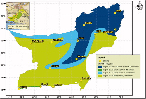
The weather of Pakistan is mainly affected by Monsoon and the Western Disturbance (Salma et al., 2012). Western Disturbances, the low-pressure cells in the Westerlies, are the source of moderate to light showers in southern areas of the country while heavy to moderate showers with substantial snowfall in the northern areas of the country occurs in the winter months typically. In almost whole Pakistan excluding Chitral, Gilgit–Baltistan, Western KPK and Western Baluchistan, Monsoon occurs in summer from June till September (Maida and Ghulam, 2011; Hanif et al., 2013; Hussain and Lee, 2014). These monsoon rains are heavy in nature and can cause significant flooding if they interrelate with western disturbance, especially in the Northern areas of the country. Tropical Storms usually form in pre-monsoon months from late April till June and then from September till November mainly affect the coastal areas. The weather of Baluchistan is mainly affected by Western Disturbances in winter and spring months. It is less affected by Monsoon in summers and to some extent with tropical storms in coastal areas in autumn (Ahmed et al. 2015; Ashraf and Routray, 2015; Aamir and Hassan, 2018; Gadiwala and Burke, 2019). Furthermore, contemporary significance of Baluchistan is far more than ever before due to Gwadar port that is the crown jewel of CPEC project. Additionally, a considerable portion of land routes of One Belt One Road (OBOR) and of CPEC is also stretches through Baluchistan terminating at the port. Therefore, conducting precipitation trend analysis on the study area is of utmost significance in this day and age.

2.2. Data sources and data processing

2.2.1. Precipitation data

Monthly Precipitation data in millimeters, for this research was acquired from Pakistan Meteorological department (PMD). Thirteen stations namely Barakhan, Dalbandin, Jiwani, Kalat, Khuzdar, Lasbella, Nokkundi, Ormara, Pasni, Punjgur, Quetta, Sibbi and Zhob throughout Baluchistan were chosen based on authentic source, completeness and availability of data. The distribution of stations in different climatic regions within Baluchistan is shown in Fig. 1. The Study period constitute of forty-one (41) years from 1977 to 2017 for the selected stations in Baluchistan. Data collected from PMD was on the monthly basis in (mm/month) for each of the weather stations and was converted into monthly means. The average monthly and annual precipitation within the study period is tabulated below in Table 1.

Table 1. Average precipitation from 1977–2017.

Red color shows the histogram of monthly precipitation among stations, brown color shows the histogram of monthly precipitations among region, green color shows seasonal whereas blue color shows annual precipitation.

Western parts of Baluchistan such as Dalbandin, Jiwani, Kalat, Nokkundi, Ormara, Punjgur, Pasni, Quetta receives most of its precipitation in Winter Season due to the western disturbance and Eastern parts of Baluchistan such as Barakhan, Khuzdar, Lasbella, Sibbi and Zhob receives its most of the precipitation in Monsoon Season (Table 1). Stations close to coastal areas also receives scattered precipitation in the post Monsoon season when continental air prevails.2.2.2. Teleconnections and climatic indices

The Large-scale teleconnections (teleconnections) are the spatial pattern in the stratosphere, showing the atmospheric and oceanic circulation. They are responsible for remote connection between weather/climate anomalies over large distances around the globe (Feldstein and Franzke, 2017). Teleconnections are persistent, they can last for short as well as long duration like one to two weeks or, inter-annual to decadal. Climatic indices are the diagnostic quantitative representation of large-scale circulation and teleconnection patterns. Climatic index of teleconnection patterns NAO, AO, AMO, IOD-DMI, IOD-EQWIN, PDO, ENSO-MEI, ENSO MODOKI (ENSO-EMI) known to have affected the precipitation in the study area through teleconnection (Liu et al., 2012; Afzal et al., 2013; Athar, 2015; Iqbal and Athar, 2018) are considered. Data of climate Indices are downloaded from NOAA-ESRL Physical Sciences Division (https://www.esrl.noaa.gov) except IOD which is downloaded from JAMSTEC (http://www.jamstec.go.jp/aplinfo/sintexf/e/index.html) and listed in Table 2. The brief description of the climate indices is provided in the following paragraph whereas the domain used to define the teleconnection pattern is provided in Table 2.

Table 2. Description of climate indices.

Climate indices	Source	Domain to define index
NAO	www.esrl.noaa.gov	Icelandic Low: 50N-320, 55N-320; 75N-360, 70N-360; approx. Azores High: 25N-315, 30N-315, 45N-355, 50N-355; approx.
AO	www.esrl.noaa.gov	Artic Poles; North of 20N
AMO	www.esrl.noaa.gov	0-60N; 280–360 approx.
DMI	www.jamstec.go.jp/aplinfo/sintexf/e/index.html	EEIO; 0-10S; 90–110 WEIO; 10N-10S; 50–70
EQWIN	www.esrl.noaa.gov	CEIO: 5N-5S; 60–90
ENSO-MEI	www.esrl.noaa.gov	30N-30S; 100–290
ENSO-MODOKI	www.esrl.noaa.gov	MODOKI-A (Right): 10N-10S; 165–240 MODOKI-B (Center): 5N-15S; 250–290 MODOKI-C (left): 20N-10S; 125–145
PDO	www.esrl.noaa.gov	Pacific Ocean; North of 20N

Table 3. Monthly significant increasing (decreasing) trends in precipitation – individual stations.

Stations	Parameters	Jan	Feb	Mar	Apr	May	Jun	Jul	Aug	Sep	Oct	Nov	Dec
Barakhan	S	−177	−70	−144	−57	−1	175	−76	44	−79	7	−211	−74
	p	4.62%	43.14%	10.57%	52.20%	99.10%	4.93%	39.33%	62.12%	37.49%	93.32%	1.07%	38.76%
	TS	−0.205*	−0.206	−0.478	−0.187	0.000	0.832*	−0.767	0.354	−0.291	0.000	0.000	0.000
Dalbandin	S	−132	−43	−79	−53	−98	−21	−42	−67	13	−24	−91	−208
	p	13.74%	62.70%	37.29%	54.73%	22.36%	76.83%	49.35%	27.46%	74.52%	71.94%	23.49%	1.64%
	TS	−0.240	−0.027	−0.113	0.000	0.000	0.000	0.000	0.000	0.000	0.000	0.000	−0.051
Jiwani	S	−13	−158	−72	−93	−30	−59	−34	−58	0	−32	−72	−245
	p	88.23%	6.31%	39.71%	19.20%	20.49%	30.99%	57.93%	41.59%	0.00%	48.30%	24.04%	0.37%
	TS	0.000	−0.002	0.000	0.000	0.000	0.000	0.000	0.000	0.000	0.000	0.000	−0.074
Kalat	S	−43	47	28	−35	23	68	−167	−68	9	−68	66	−114
	p	62.89%	59.72%	75.22%	69.12%	78.48%	39.87%	5.41%	43.02%	89.95%	28.97%	42.94%	18.86%
	TS	−0.079	0.130	0.004	0.000	0.000	0.000	−0.117	0.000	0.000	0.000	0.000	−0.049
Khuzdar	S	−97	−67	28	−47	28	31	−20	−59	30	−93	−151	−178
	p	27.45%	45.12%	75.27%	59.65%	75.21%	72.56%	82.22%	50.75%	73.06%	21.50%	6.45%	4.01%
	TS	−0.117	−0.242	0.092	−0.011	0.000	0.000	−0.067	−0.380	0.000	0.000	0.000	−0.094
Lasbella	S	9	−120	58	41	133	78	−92	−60	105	−84	−90	−57
	p	91.68%	16.84%	50.54%	63.79%	13.09%	37.58%	29.86%	49.69%	16.15%	23.88%	19.32%	39.36%
	TS	0.000	−0.046	0.000	0.000	0.292	0.004	−0.225	−0.150	0.000	0.000	0.000	0.000
Nokkundi	S	62	8	−2	12	20	59	−48	−63	0	39	−26	−72
	p	47.94%	92.72%	98.19%	87.98%	77.89%	24.13%	34.06%	11.52%	0.00%	52.48%	68.56%	37.15%
	TS	0.000	0.000	0.000	0.000	0.000	0.000	0.000	0.000	0.000	0.000	0.000	0.000
Ormara	S	−19	−28	−73	−67	−205	108	82	66	5	−407	−20	−19
	p	82.81%	74.38%	37.14%	31.60%	0.63%	7.82%	30.15%	35.46%	92.09%	0.01%	69.13%	82.32%
	TS	0.000	0.000	0.000	0.000	0.000	0.000	0.000	0.000	0.000	−0.005	0.000	0.000
Panjgur	S	−28	−93	−56	−32	135	18	−195	−78	−5	−76	−90	−176
	p	75.17%	29.40%	52.60%	70.43%	8.89%	80.07%	2.28%	31.75%	93.79%	13.13%	17.80%	3.51%
	TS	0.000	−0.131	−0.019	0.000	0.000	0.000	−0.083	0.000	0.000	0.000	0.000	0.000
Pasni	S	−52	−64	−60	0	−35	15	10	−116	6	−50	49	−91
	p	55.68%	46.03%	48.35%	100.00%	38.15%	81.53%	89.61%	12.19%	89.54%	27.30%	42.43%	28.44%
	TS	−0.006	0.000	0.000	0.000	0.000	0.000	0.000	0.000	0.000	0.000	0.000	0.000
Quetta	S	−224	−44	−157	130	165	206	−33	−12	153	8	76	−169
	p	1.19%	62.11%	7.78%	14.38%	6.07%	1.26%	70.15%	88.99%	3.14%	91.50%	37.77%	5.74%
	TS	−1.223*	−0.265	−0.966	0.200	0.019	0.000	0.000	0.000	0.001	0.000	0.000	−0.543
Sibbi	S	−69	23	−91	−42	154	186	22	21	153	−57	−61	−63
	p	43.55%	79.55%	30.66%	62.80%	6.78%	2.59%	80.46%	81.35%	6.70%	32.66%	43.44%	45.50%
	TS	−0.031	0.000	−0.185	0.000	0.000	0.000	0.042	0.069	0.000	0.000	0.000	0.000
Zhob	S	−201	−19	−132	−39	38	161	56	−122	77	−38	−39	−160
	P	2.39%	83.08%	13.81%	66.12%	66.85%	7.04%	52.93%	17.06%	38.20%	61.98%	64.03%	6.63%
	TS	−0.417*	−0.029	−0.655	−0.078	0.044	0.250	0.264	−0.559	0.029	0.000	0.000	−0.056

Figures in bold represents significant correlations at 5% confidence level. * shows noteworthy Theil Sen Slope (TS). Where S is Mann Kendall statistic, p is significance probability (p-value) and TS is Theil Sen Slope.

The North Atlantic Oscillation (NAO) index is based on the sea-level surface pressure anomaly between the Subtropical (Azores) High and Sub polar (Iceland) Low. In the positive (stronger) phase above-normal pressure over the Azores and below normal pressure over Iceland prevails. In negative phase weak high pressure over Azores and weak low pressure over Iceland prevails. The Positive phase leads to increased westerlies which follows the northern track resulted in cool summers and mild, wet winters in Central Europe. The negative phase of NAO leads to suppressed westerlies, and as a result northern European area suffer cold dry winters. The storms track southwards toward the Mediterranean Sea and much into northern Asia.

The Arctic Oscillation (AO) is a form of atmospheric circulation over the Northern Hemisphere, particularly from mid-to high. In positive phase low air pressure on the Arctic and high air pressure over the Atlantic Oceans and Northern Pacific is observed. The regions on the mid-latitudes experience less cold air outbreaks (CAOs). Positive phase is associated with strong polar vortex which constrained the cold Arctic air to North. Jet stream remains zonal and storm tracks in North East direction. During the negative phase, higher air pressure on the Arctic and lower air pressure over the Atlantic Oceans and Northern Pacific is observed. Negative phase is associated with weaker polar vortex allows the cold air to invade USA and Europe. The regions on mid-latitudes can undergo waves of chilly air. Jet stream takes more meridional path with trough over USA/Europe and crest over North Atlantic. Storms follows more direct and East ward path often called Nor’easters.

The Atlantic Multi-decal Oscillation (AMO) is characterized by an SST anomaly in the North Atlantic and consists of the warm phase and cool phases with periods of 20–40 years approximately. From early 1960s to the mid 1990s AMO index shows a relatively cool phase, and from 1997 AMO has been in a warm phase. AMO has positive correlation with the monsoon rainfall. The AMO may influence the monsoon through the summer North Atlantic oscillation (NAO) and further through the equatorial zonal winds increasing the moisture flow over the sub-continent region by enhancing the southwesterly flow.

The Dipole Mode Index (DMI) is the ocean segment of Indian Ocean Dipole (IOD) and depends solely on Sea Surface Temperature (SST) inconsistencies. DMI estimates the contrast between SST peculiarities in 02 locales of IOD: West Equatorial Indian Ocean (WEIO), 50°E-70°E and 10°S-10°N and East Equatorial Indian Ocean (EEIO): 90°E −110°E and 10°S-0°. During the positive phase, water in the eastern region is cooler and it is warmer in the western Indian Ocean as compared to the usual temperature. This positive phase benefits the sub-continent region by directing Monsoon towards it. During the negative phase, water in the eastern region is warmer and it is cooler in the western Indian Ocean as compared to usual the temperature. This negative IOD has been found over the study area during several dry spell years.

Equatorial Indian Ocean Oscillation (EQUINOO) is the atmospheric segment of IOD and is the fluctuation of atmospheric cloudiness between the Eastern Equatorial Indian Ocean (EEIO) & Western Equatorial Indian Ocean (WEIO). The index that describe EQUINOO is EQWIN which is the negative of the standardized zonal wind anomaly over the Central Equatorial Indian Ocean (CEIO) region. The EQWIN index is highly correlated with the difference between the OLR of WEIO and EEIO. In the Positive phase of EQUINOO, enhanced cloudiness is observed over the WEIO as compared to the EEIO and was favorable to the Monsoon. A favorable EQUINOO is believed to have effects on the influence of the El-Nino through tele-connection.

The periodic variability every 2 to 7 years in sea surface temperature (El Niño) and the air pressure of the superimposing atmosphere (Southern Oscillation across the equatorial Pacific Ocean is called ENSO. El Niño and its contrary La Niña both have a disturbing effect on Monsoon Climatic condition in many different parts of the world as well. Tropical Pacific’s 6 important parameters, namely sea surface temperature (S), sea-level pressure (P), surface air temperature (A), zonal (U) and meridional (V) components of the surface wind and lastly the total cloudiness fraction of the sky (C) combine together to form the Multivariate ENSO Index MEI, which incorporates most information than any other indices.

ENSO Modoki Index (EMI-MODOKI) describe the distinctive SST anomalies in tropical Pacific Ocean. It has two phases La Nina Modoki: colder central Pacific flanked by warm eastern and western Pacific, El Nino Modoki: warm anomaly of the central Pacific when bordered by cold anomalies on both east and west sides of the ocean. Latest research reveals that ENSO Modoki has distinct teleconnections that has far flung reaching influences. It even affects the precipitation over sub-continent and South Africa.

The Pacific Decadal Oscillation (PDO) is the common climate disparity in the SST and SLP of the Pacific basin adjacent to North America. It has two phases: warm or cold that may last for 20 to 30 years. During positive phase SLPs are below average over the North Pacific or SSTs are inconsistent cool in the interior North Pacific and warm along the Pacific Coast of North America. During negative phase SLPs over the North Pacific is above average or warm SST anomalies in the interior and cool SST anomalies along the North American coast prevails.

2.2.3. Climate variables

Atmospheric and oceanic climate variables such as Sea Surface Temperature (SST), Sea Level Pressure (SLP), Zonal Winds at surface (ZW-Surface) and Geo-potential Heights at 500 hpa level (GPH500) are considered to determine Empirical Orthogonal Maps (EOF) and their relationship with the precipitation variability. HADISST v1.1 1 × 1 degrees gridded data are downloaded from Met Office Hadley Center (https://climatedataguide.ucar.edu/climate-data/sst-data-hadisst-v11.) whereas NCEP/NCAR Reanalysis 2.5 × 2.5 degree gridded data of SLP, GPH, Zonal Wind and OLR are downloaded from the NOAA-ESRL Physical Sciences Division website (https://www.esrl.noaa.gov).

2.3. Statistical analysis

Trends are examined using Mann-Kendall Tests in the monthly time series precipitation data of each of 13 stations. The slope of the trend is calculated using Theil Sen’s Slope which is recommended for metrological analysis (Gujarati, 2009). The influence of climate indices on precipitation trends is assessed by the Partial Mann-Kendall test. The analysis is performed on individual stations for monthly time series data. Empirical Orthogonal Function (EOF) and principal component analysis (PCA) is used for calculating the precipitation variability in Baluchistan Region. The association between precipitation-climate indices and precipitation-climatic variables is determined by Pearson’s correlation (Zhang et al., 2017).

2.3.1. Mann-Kendall for trend detection

The Mann-Kendall (MK) test was largely used in identifying trends in climate variables (Libiseller and Grimvall, 2002; Bastiaanssen and Ali, 2003; Arif et al., 2004; Webster et al., 2011; Kreft and Eckstein, 2013; Ahmad et al., 2015; Eckstein et al., 2019; Naz et al., 2020). The MK test is a non-parametric test based on ranks and is not sensitive to sudden breaks in the uneven data. The reasons for adopting the Mann-Kendall test is that it is strong and insensitive to the data with gaps and best for the data that is not normally distributed. The MK test is one of the strong methods of identifying monotonic trends in precipitation data where the data is skewed and/or where data is either consistently increasing or decreasing in a time series and is not suitable when there are recurring trends. The Mann-Kendall statistic S_x of the series x is given (Yue et al., 2002) as: $$S_x=\sum _{i-l}^{n-1}\sum _{j=i+l}^n\mathit{sgn}(X_j-X_i)$$ $$\mathit{sgn}(X_j-X_i)=\{\begin{array}{c}+1\hspace{0.5em}(X_j-X_i)>0\\ 0\hspace{0.5em}\text{if}\hspace{0.5em}(X_j-X_i)=0\\ -1\hspace{0.5em}(X_j-X_i)<0\end{array}$$ where, i and j are the rank of observation of the Xi and Xj of the time series. The variance associated with S_x is given as $$\mathit{Var}=\frac{n(n-1)(2n+5)-{\sum }_{i=1}^g{t}_i(t_i-1)(2t_i+5)}{18}$$ where g is the groups of tied rank and t is ties in the group. For a sample size of n > 10 or larger, the MK statistics Z_mk is computed by $$Z_{mk}=\{\begin{array}{c}\frac{S_x-1}{\sigma }\\ \frac{S_x+1}{\sigma }\\ 0\end{array}\hspace{0.5em}\begin{array}{c}\mathit{for}\hspace{0.5em}{S}_x>0\\ \mathit{for}\hspace{0.5em}{S}_x<0\\ \mathit{for}\hspace{0.5em}{S}_x=0\end{array}$$

Positive Z_mk values show increasing trends, while negative Z_mk values reflect decreasing trends. If |Z_mk| is greater than Z_1-α/2 for the chosen value of significance level (α) then the trends are considered significant or when p-value is smaller than the significance level (α), the null hypothesis (H_o) of no trend is rejected in favor of the alternative hypothesis (Ha) and the trend is considered as a significant trend in the time series. Z_1-α/2 and p-value are obtained from the standard normal distribution table.

2.3.2. Theil Sen’s slope (TS)

TS is used to compute the magnitude of the trend. It is more robust than the linear regression since it limits the influence of outliers and performs better even for the case of normally distributed data (Gujarati, 2009; Chervenkov and Slavov, 2019). According to TS method, the overall slope S* is the median of N values of slope S and is given by $$S^{*}=\frac{S_{N+1}}{2},\hspace{0.5em}If\hspace{0.5em}N\hspace{0.5em}is\hspace{0.5em}\mathit{odd}$$ $$S^{*}=\frac{S_{\frac{N}{2}}+S_{\frac{N+2}{2}}}{2},\hspace{0.5em}If\hspace{0.5em}N\hspace{0.5em}is\hspace{0.5em}\mathit{even}$$ where, S is the slope between any two values of a time series x. For a time series x having n observations, there are a possible N = n*(n-1)/2 values of S that can be calculated using $$S=\frac{x_k-x_j}{k-j},\hspace{0.5em}\mathit{where}\hspace{0.5em}k\ne j$$

2.3.3. Partial Mann-Kendall for examining the influence of climatic indices on precipitation trends

The influence of large-scale climate indices on the precipitation time series is examined by partial Mann-Kendall (PMK) test (Libiseller and Grimvall, 2002; Yue et al., 2002; Libiseller, 2004; Ahmad et al., 2015; Iqbal and Athar, 2018). PMK is one of the best one step procedures that do the adjustment for covariates (influencing variables) and trend testing simultaneously. Pearson correlation measures the strength of linear association between two variables. PMK is another approach to study the changes in trends in precipitation in the presence of climate indices which are the covariates. Trends in precipitation (response variable) can be assessed in the presence of the relevant covariates through PMK when the effect of the explanatory variable is removed (Libiseller and Grimvall, 2002). In PMK, the effect of explanatory variables is studied on the response variable and the influence is calculated using the conditional mean and the conditional variance of the response variable. The test statistic for response variable y, with its covariate x being the explanatory variable is given by $$\mathit{PMK}=\frac{S_y-\stackrel{⌢}{\rho }{S}_x}{\sqrt{(1-\stackrel{⌢}{\rho })}n(n-1)(2n+5)/18}$$ where, S_y is the Mann-Kendall statistics of response variable, S_x is the Mann-Kendall statistics of explanatory variable, $\stackrel{⌢}{\rho }$ denotes the conditional correlation between the MK statistics S_x and S_y. The PMK statistic is normally distributed with mean 0 and standard deviation 1.

Multicollinearity, if present in variates then it reduces the precision of the estimate of coefficients and weakens the statistical power of the regression model. In case of multi collinear variates, PMK method is different from Multiple linear regression (Dogar et al., 2017; Dogar and Sato, 2018, 2019) in the sense that PMK method doesn’t account for the dependence or influence of one variable on the other as it treats each input variable separately.

2.3.4. Empirical orthogonal analysis or principal component analysis

Empirical Orthogonal Analysis also called as the Principal Component Analysis finds the independent orthogonal variables (EOFs) that describe the maximum variability of a two-dimensional data set. First dimension being the spatial location in which the EOF is being found and the second dimension is the time, which represents the dimension in which realizations of this structure are sampled. EOF analysis is performed on precipitation and climate variables to determine the influencing climate indices of large-scale teleconnection patterns. Mathematical expression is provided in appendix B1.

3. Results and discussions

3.1. Spatial and temporal trends in precipitations

Monotonic Trends in monthly precipitation from 1977 to 2017 at 13 stations of Baluchistan are found through Mann-Kendall tests at individual stations. Out of 15 statistically significant trends, 10 were decreasing trends whereas 5 were increasing trends (Table 3). This indicates that decreasing trend is dominating in most of the stations in Baluchistan, which explains the declining precipitation occurrences in Baluchistan during the last couple of decades. The slope of the significant trend is calculated by the TS method.The TS of the significant trends in the Table 3 which are noteworthy are shown with ‘*’ whereas others although their trends are significant, but their slopes are almost flat can be ignored. Therefore, it can be inferred that generally the decreasing trends of precipitation in January are dominant with a noticeable average slope of 0.615 mm/year whereas increasing trends of precipitation in June are prevailing with a noticeable average slope of 0.832 mm/year. The average precipitation in the month of January and June is 18.7 mm and 11.8 mm (Table 1) respectively. Thus, a significant decreasing trend having slope 0.615 mm/year in January is quite obvious which may create dryness whereas significant increasing trend in June having slope 0.832 mm/year may create some heavy downpour conditions respectively. It may also be noted that the significant trend (increasing/decreasing) is found in stations located in Region1. On the contrary no trend, is found in stations located regions 2,3 and 4.

3.2. Influence of climatic indices on precipitation trends

The climatic indices pertinent to Baluchistan which would have influenced these decreasing (increasing) precipitation trends in January (June) are determined. The changes in precipitation trends in the presence of influencing variables NAO, AO, AMO, IOD-DMI, IOD-EQWIN, PDO, ENSO-MEI and EMI-MODOKI is determined through the PMK on monthly precipitation at individual station and is tabulated in the Tables A2–A9. The Influence determined through the PMK is classified in to weak, moderate and strong influence as described in the Table A1. The results of the variation in precipitation trends for the significant decreasing (increasing) trends of January (June) are tabulated in Table 4. It can be seen from the Table 4 that all the climatic variables mentioned above have weak influence on precipitation trends except EQWIN and ENSO-MEI and EMI-MODOKI which have moderate to strong influence on precipitation trends.

Table 4. Influence of climatic variables on precipitation trends.

Months	Stations	NAO	AO	AMO	DMI	EQWIN	PDO	MEI	EMI-MODOKI
January	Barakhan	Weak (−)	Weak (−)	Weak (−)	Weak (−)	Strong (−)	Weak (−)	Weak (−)	Strong (−)
	Quetta	Weak (−)	Weak (−)	Weak (−)	Weak (−)	Moderate (−)	Weak (−)	Weak (−)	Strong (−)
	Zhob	Weak (−)	Weak (−)	Weak (−)	Weak (−)	Strong (−)	Weak (−)	Moderate (−)	Strong (−)
June	Barakhan	Weak (+)	Weak (+)	Weak (+)	Weak (+)	Strong (+)	Weak (+)	Weak (+)	Strong (+)

(+ve) shows increasing trends whereas (-ve) shows decreasing trends.

Table 10. Region1 precipitation modes (EOFs) and corresponding PCs for the month June.

EOFs	Variability explained	Cumulative	PCs	Correlation coeff.	p-value
EOF1	58.61%	58.61%	PC1	0.7793	0.0001
EOF2	16.19%	74.80%	PC2	−0.5306	0.0003
EOF3	16.02%	90.82%	PC3	0.1521	0.3425
EOF4	5.68%	96.50%	PC4	−0.1578	0.3246
EOF5	3.50%	100.00%	PC5	−0.2188	0.1693

Bold figure represents significant correlations at 5% confidence and the shaded rows indicated the selected modes.

Table A1. Classification of influence type.

S. No	Condition	Statistical significance of trend	Influence type
1	MK shows insignificant trend; after conditioning of influencing variable through PMK, the trend still remained statistically insignificant	Insignificant	Insignificant
2	MK shows insignificant trend; after the conditioning of influencing variable through PMK, the trend becomes statistically significant	Significant	C1, C2 or C3
3	MK shows significant trend, ; after the conditioning of influencing variable through PMK, the trend further amplified and becomes more statistically significant	Significant	C1, C2 or C3
4	MK shows significant trend, ; the conditioning of influencing variable through PMK, the trend becomes statistically insignificant	Significant	C1, C2 or C3
C1	PMK Conditioning of influencing variable changes the MK-Statistics by up to 5%.	Significant/Insignificant	Weak
C2	PMK Conditioning of influencing variable changes the MK-Statistics from 5% to 10%.	Significant/Insignificant	Moderate
C3	PMK Conditioning of influencing variable changes the MK-Statistics more than 10%.	Significant/Insignificant	Strong

3.3. Influence of climate indices on precipitation variability

It is found through MK and TS that precipitation trends are significant in the month of January and June. The stations in which the precipitation trends came out significant situated in the Region1 of Baluchistan. As it can be seen in Table 1, Region1 comparatively receives a larger portion of Baluchistan precipitation whereas other regions receive less precipitation and remain dry. It can also be seen in Table 1 that the major share of precipitation is in winter (December, January and February) followed by Monsoon (June, July, August and September) in summer. As such, we focus our attention on to the month of January (June) in which the stations in Region1 show decreasing (increasing) trends in order to determine the relationship of this precipitation variability with the teleconnection patterns. The influence of teleconnection patterns on the January (June) precipitation variability is determined through the following steps

1. Variability patterns (modes) in the Region1 precipitation are identified through principal component analysis and their corresponding time series (PCs) are constructed

2. Correlation analysis is performed between time series of Region1 precipitation (PCs.) and climate Indices to check their relevance.

3. EOF analysis is performed on SST, SLP and ZW-Surface to find out the dominated teleconnection patterns prevailing in the months of January and June which may have influenced the precipitation of Region1 in Baluchistan and explains the precipitation variability.

4. Correlation analysis is performed between time series of Region1 precipitation and SST anomalies, atmospheric circulations such as SLP, Geopotential Heights (500 hpa), Zonal winds (surface), OLR to observe their relationship and influence with Region1 precipitation.

3.4. Linkages of January precipitation variability with climate indices

3.4.1. Modes of Region1 precipitation for the month of January

PCA is performed on the R1JANP for the period 1977 to 2017. First three (3) EOFs explain 88.7% variation, capable enough to explain the precipitation variability in Region1 (Table 5) and these three (3) PCs are then used to perform the correlation analysis with climate indices. The correlation between time series of PCs and R1JANP is shown in Table 5. The selected PCs are shown as highlighted. The spatial and temporal distribution of Region 1 precipitation, EOFs and PCs are shown in Appendix C.

Table 5. Region1 Precipitation Modes (EOFs) and Corresponding PCs for the Month January.

EOFs	% Variability explained	Cumulative	PCs	Correlation Coeff.	p-value
EOF1	53.80%	53.80%	PC1	0.972	0.001
EOF2	18.75%	72.55%	PC2	0.177	0.267
EOF3	16.15%	88.70%	PC3	0.142	0.375
EOF4	6.94%	95.64%	PC4	−0.024	0.882
EOF5	4.36%	100.00%	PC5	−0.047	0.768

Bold figure represents significant correlations at 5% confidence and the shaded rows indicated the selected modes.

3.4.2. Correlation of Region1 precipitation for the month of January with climate indices

In order to find out the association of R1JANP with climate indices, correlation is performed between time series of Region1 precipitation PC (R1JANP-PCs) and the climate indices for the respective month of January. The results are presented in Table 6. Large scale teleconnection circulation patterns NAO and AO shows insignificant correlation with Region1 precipitation. Atlantic Multi Decadal Oscillation index (AMO) is positively correlated to PC3 at 7.91% confidence. Indian Ocean Dipole mode index DMI is positively correlated to PC2 at 12.39% confidence. Indian Ocean Circulation pattern defined by EQWIN is significant at 1.15% and positively correlated to PC1. Large scale Teleconnection pattern ENSO-MEI is negatively correlated to PC2 at 16.52% confidence. ENSO-MODOKI Index (EMI-MODOKI) is positively correlated to PC2 at 21.81% confidence whereas it is positively correlated to PC3 at 4.82% confidence also. Pacific Ocean decadal oscillation (PDO) is negatively correlated to PC1 at 20.51% confidence.

Table 6. Correlation between R1JANP-PCs and climate indices.

Indices	R1JANP-PC1		R1JANP-PC2		R1JANP-PC3
	Corrl. coeff.	p-value	Corrl. coeff.	p-value	Corrl. coeff.	p-value
NAO	−0.1488	0.3532	−0.1284	0.4236	−0.1039	0.5178
AO	0.0517	0.7483	−0.1479	0.3561	0.1278	0.4258
AMO	−0.1020	0.5257	0.0269	0.8674	0.2774	0.0791*
DMI	0.0546	0.7345	0.2442	0.1239	−0.0698	0.6644
EQWIN	0.3758	0.0155*	−0.1089	0.4981	0.0352	0.8271
ENSO-MEI	0.0102	0.9497	−0.2209	0.1652	−0.1444	0.3678
EMI-MODOKI	−0.0948	0.5554	0.1966	0.2181	0.3105	0.0482*
PDO	−0.2021	0.2051	−0.0328	0.8386	−0.0924	0.5654

Bold with asterick figures indicate significant correlation at 7% confidence whereas highlighted figures indicate correlation up to 20% confidence.

3.4.3. Leading modes of teleconnection patterns for the month of January

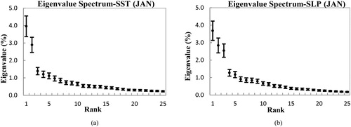
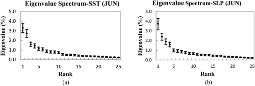
EOF analysis is performed on SST, SLP and ZW-Surface for the month of January. The leading modes of EOFs are selected based on their distinguishability within their uncertainties. The non-degeneracy of eigen-spectrum is an important property and can be used for the selecting leading modes of EOFs. The uncertainty estimates of January eigenvalues spectrum of covariance matrix of SST and SLP are calculated by North et al. (1982) rule of thumb. Two eigenvalues of SST and three eigenvalues of SLP are well distinguishable from the rest of the spectrum as shown in Fig. 2a,b. Therefore, three leading modes for each of teleconnection patterns are considered for the analysis.

Fig. 2. (a) Eigenvalue spectrum (%) of the covariance matrix of January SST. The vertical bar shows uncertainty estimates based on North et al. (1982) rule of thumb. The leading 25 eigenvalues out of 41 are shown. (b) Eigenvalue spectrum (%) of the covariance matrix of January SLP. The vertical bar shows uncertainty estimates based on North et al. (1982) rule of thumb. The leading 25 eigenvalues out of 41 are shown.

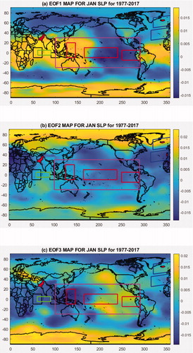
Leading three modes EOF1(18%), EOF2(13%) and EOF3(6%) of SST explained about 37% cumulative variability and shows the patterns of PDO in North Pacific Ocean, EL-NINO, EMI-MODOKI (warm center flanked by cold sides or vice-versa) in Central Pacific Ocean, DMI pattern (though weak) in Indian Ocean whereas AMO and NAO (associated SST pattern) in North Atlantic Ocean. Leading modes of SST are shown in Fig. 3a–c, respectively. Fig. 4a–c shows three leading modes of SLP. EOF1 (17%), EOF2 (13%), EOF3 (11%) of SLP explained about 41% cumulative variability and shows the patterns of ENSO, NAO and AO. EOF1 of SLP shows anti-cyclonic circulation over Region1 indicative of negative association with influencing indices whereas EOF2, EOF3 show cyclonic circulation indicative of positive association with influencing indices.

Fig. 3. EOFs of standardized SST for January over 1977–2017. (a) EOF1 shows the pattern of ENSO and PDO in Pacific Ocean. (b) EOF2 shows the pattern of AMO in Atlantic Ocean and pattern of DMI in Indian Ocean. (c) EOF3 shows PDO, EMI-MODOKI and NAO (SST associated pattern). Black boxes show Western Equatorial Indian Ocean (WEIO) and Eastern Equatorial Indian Ocean (EEIO) region whereas green box shows Central Equatorial Indian Ocean (CEIO) region in Indian Ocean. Red boxes show ENSO-MODOKI regions whereas magenta box shows ENSO-MEI region in Pacific Ocean. Blue boxes show NAO region in Atlantic Ocean.

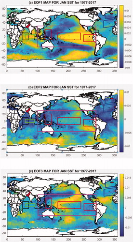
Fig. 4. EOFs of standardized SLP for January over 1977–2017. (a) EOF1 shows the pattern of ENSO-SOI and NAO pattern though not very distinguished. (b) EOF2 shows the pattern of AO. (c) EOF3 shows patterns of ENSO and NAO pattern though not very distinguished. Black boxes show Western Equatorial Indian Ocean (WEIO) and Eastern Equatorial Indian Ocean (EEIO) region whereas green box shows Central Equatorial Indian Ocean (CEIO) region in Indian Ocean. Red boxes show ENSO-MODOKI regions whereas magenta box shows ENSO-MEI region in Pacific Ocean. Blue boxes show NAO region in Atlantic Ocean.

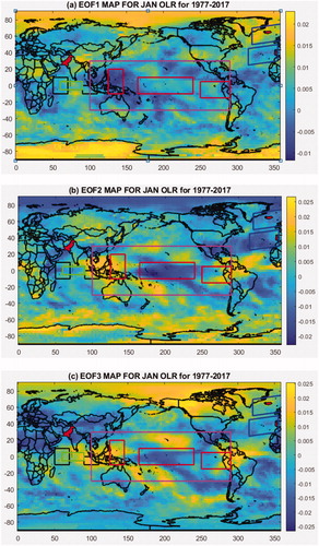
Leading modes of ZW-Surface are shown in Fig. 5a–c, respectively. EOF1(10%), EOF2(7%) and EOF3(6%) of ZW-Surface explained about 23% cumulative variability. Since EQWIN is highly correlated with the difference of Outgoing Longwave Radiation (OLR) in Eastern Equatorial Indian Ocean (EEIO) and Western Equatorial Indian Ocean (WEIO) regions therefore the occurrence of EQWIN can easily be detected by identifying the enhanced/suppressed convection (cloudiness) in WEIO/EEIO region. EOFs of OLR are shown in Fig. 6a–c. EOF1 and EOF3 show weak whereas EOF2 shows moderate pattern of EQWIN.

Fig. 5. EOFs of standardized SZW for January over 1977–2017. (a) EOF1 shows weak patterns of EQWIN. (b) EOF2 shows moderate pattern of EQWIN whereas (c) EOF3 shows weak patterns of EQWIN. Black boxes show Western Equatorial Indian Ocean (WEIO) and Eastern Equatorial Indian Ocean (EEIO) region whereas green box shows Central Equatorial Indian Ocean (CEIO) region in Indian Ocean. Red boxes show ENSO-MODOKI regions whereas magenta box shows ENSO-MEI region in Pacific Ocean. Blue boxes show NAO region in Atlantic Ocean.

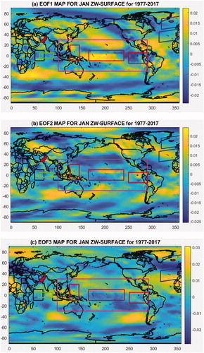
Fig. 6. EOFs of standardized OLR for January over 1977–2017. (a) EOF1 shows weak patterns of EQUINOO. (b) EOF2 shows moderate pattern of EQUINOO whereas (c) EOF3 shows weak patterns of EQUINOO. Black boxes show Western Equatorial Indian Ocean (WEIO) and Eastern Equatorial Indian Ocean (EEIO) region whereas green box shows Central Equatorial Indian Ocean (CEIO) region in Indian Ocean. Red boxes show ENSO-MODOKI regions whereas magenta box shows ENSO-MEI region in Pacific Ocean. Blue boxes show NAO region in Atlantic Ocean.

From the EOF analysis as above, it is clear that patterns of NAO (weak), AO (moderate to weak), AMO (moderate), DMI (moderate), EQWIN (moderate), ENSO-MEI (moderate), EMI-MODOKI (strong) and PDO (moderate) are found in the three leading modes of January.

3.4.4. Relationship of Region1 precipitation with SST anomalies for January

Figure 7 below shows the distribution of correlation coefficient between PCs (1, 2 and 3) and standardized SST for the month of January. In tropical areas, PC-1 is positively correlated with central-Eastern pacific whereas it is negatively correlated with western pacific (Fig. 7a). This surface SST anomaly is indicative of linkages of precipitation with ENSO-MEI, but the correlation is mostly insignificant with some significant areas and may be considered as weak which is in line with the findings in Table 6. Figure 7b,c show negative correlation in the central area for EMI-MODOKI and positive correlation in flank areas marked by red boxes, which is indicative of linkages of PC2 and PC3 with the EMI Index. At mid and high latitudes, PC3 is negatively and positively correlated with SSTs analogous to PDO index (Fig. 7c).

Fig. 7. Correlation between PCs of Region1 precipitation and standardized SST for January over 1977–2017. (a) PC1 shows weak correlation with DMI. (b) PC2 shows moderate correlation with DMI and weak correlation with EMI-MODOKI. (c) PC3 shows weak correlation with NAO and DMI, moderate correlation with AMO, EMI-MODOKI and PDO. Black boxes show Western Equatorial Indian Ocean (WEIO) and Eastern Equatorial Indian Ocean (EEIO) region whereas green box shows Central Equatorial Indian Ocean (CEIO) region in Indian Ocean. Red boxes show ENSO-MODOKI regions whereas magenta box shows ENSO-MEI region in Pacific Ocean. Blue boxes show NAO region in Atlantic Ocean.

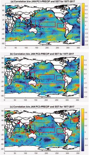
In tropical Indian ocean, PC1 is negatively correlated with SST. PC2 and PC3 are positively correlated with SST in Western Equatorial Indian Ocean (WEIO) and negatively correlated with SST in Eastern Equatorial Indian Ocean (EEIO) regions which is indicative of linkages with IOD-DMI, but the correlation appears moderate to weak with some significant positive correlated areas.

In Northern Atlantic Ocean, PC1 and PC2 (Fig. 7a,c) correlations with SST anomalies are analogous to the NAO associated SST pattern, thus indictive of association with NAO. Figure 7c shows positive correlation with SST in Northern Atlantic which is indicative of AMO linkage with PC3.

3.4.5. Relationship of Region1 precipitation with atmospheric circulation anomalies for January

The relationship of Region1 precipitation with atmospheric circulations is studied by conducting the correlation analysis between PCs and atmospheric circulations SLP, GPH500. Figure 8 below shows the distribution of correlation coefficient between PCs (1, 2, 3) and standardized SLP for the month of January. In tropical region, the pacific warm pool remains stabilized and does not show any significant correlation with Region1 precipitation. Responding to PC1, the center tropical region shows negative correlation with SLP and positive correlation in flank areas marked by red boxes. This surface SLP anomaly is indicative of linkages with ENSO-MODOKI, but the correlation is mostly insignificant with some significant areas. PC3 shows positive correlation over most of the tropical region with significant positive correlations in central tropics and negative correlation in flank areas marked by red boxes which is la-Nina EMI-MODOKI pattern.

Fig. 8. Correlation between PCs of Region1 precipitation and standardized SLP for January over 1977–2017. (a) PC1 with SLP. (b) PC2 with SLP. (c) PC3 with SLP. Black boxes show Western Equatorial Indian Ocean (WEIO) and Eastern Equatorial Indian Ocean (EEIO) region whereas green box shows Central Equatorial Indian Ocean (CEIO) region in Indian Ocean. Red boxes show ENSO-MODOKI regions whereas magenta box shows ENSO-MEI region in Pacific Ocean. Blue boxes show NAO region in Atlantic Ocean. Red ‘+’ and Black ‘.’ stipples show significant positive and negative correlation at 5% confidence, respectively.

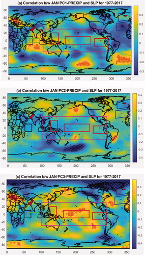
In Indian ocean, responding to SLP, PC1 shows significant positive correlation while PC-2 remains negatively correlated both without showing any distinguishable opposite anomalies similar to DMI. However, PC-3 exhibits slightly insignificant positive and negative anomaly between Western Equatorial Indian Ocean (WEIO) and Eastern Equatorial Indian Ocean (EEIO) region similar to DMI pattern.

In Northern Atlantic Ocean, high pressure anomaly is present over Iceland whereas significant low-pressure anomaly is present over Azores in response to correlation of PC1 with SLP. This surface SLP anomaly is indicative of strong (-) NAO pattern. This NAO anomaly is also accompanied by a low-pressure anomaly over Artic and high-pressure anomaly in northern Atlantic and Pacific Ocean analogous to + AO pattern but the correlation remains insignificant (weak). Responding to SLP, PC2 is positively correlated with Azores region and negatively correlated with Iceland region but the correlations remain insignificant (moderate to weak). This SLP anomaly is indicative of + NAO mode. PC2 correlation with SLP does not show any distinguishable anomaly pattern similar to + AO pattern in Arctic. PC3 again shows positive correlation with Azores and negative correlation with Iceland with insignificant correlations (moderate to weak). But responding to SLP, strong Low-pressure anomaly exist with significant negative correlation and high-pressure anomalies with significant positive correlation in Northern Atlantic and insignificant positive correlation in North Pacific Ocean somewhat similar to + AO mode.

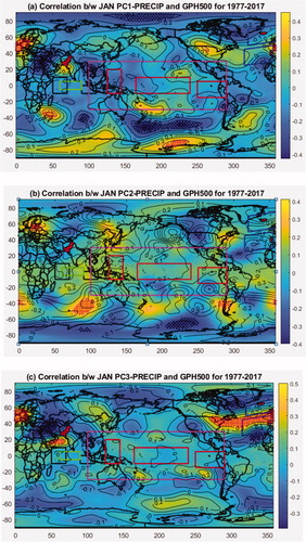
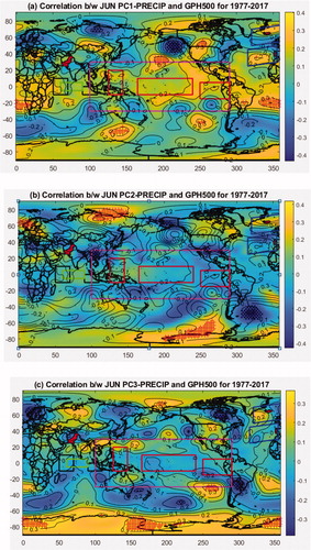
In order to understand the linkages of the observed signals of teleconnection including EMI-MODOKI, ENSO-MEI in Pacific Ocean, DMI in Indian Ocean, NAO, AO in Atlantic Ocean with Region1 precipitation through atmospheric circulations, the correlation of PCs (1, 2, 3) is performed with GPH500 as shown in Fig. 9. The precipitation favorable counter part of surface low pressure is high pressure at mid troposphere (500 hpa) which is indicative of cyclonic circulation whereas the high pressure at surface and low pressure at mid troposphere (500 hpa) is indicative of anti-cyclonic circulations. In response to correlations of PC1 with SLP and GPH500, Fig. 8a shows low surface pressure at region1 whereas Fig. 9a depicts positive height anomaly (at GPH500) which is indicative of cyclonic conditions. Positive/negative SLP anomaly in Iceland/Azores with its counterpart negative/positive anomaly at 500 hpa extending all the way to Mediterranean and Middle East Region which is indicative of linkages with NAO. Further in the tropical pacific region positive/negative/positive SLP anomaly with its counterpart negative/positive/negative in EMI-MODOKI regions indicative of teleconnection with EMI-MODOKI Index. However, cyclonic condition exists in Indian Ocean represented by high SLP anomaly and low mid altitude anomaly at 500 hpa. For PC2 correlations with responding SLP and GPH500, Figs. 8b and 9b shows that the pressure conditions at surface is not supportive of its counterpart pressure conditions at mid altitude. Lastly, for PC3 correlations with SLP and GPH500, Figs. 8c and 9c shows anti-cyclonic conditions over Region1 in response to anti-cyclonic condition at SLP and cyclonic condition at mid heights over tropical Indo-pacific region and north Atlantic region which is indicative of reduced precipitation.

Fig. 9. Correlation between PCs of Region1 precipitation and standardized GPH500 for January over 1977–2017. (a) PC1 with GPH500. (b) PC2 with GPH500. (c) PC3 with GPH500. Black boxes show Western Equatorial Indian Ocean (WEIO) and Eastern Equatorial Indian Ocean (EEIO) regions. Black boxes show WEIO and EEIO region whereas green box shows Central Equatorial Indian Ocean (CEIO) region in Indian Ocean. Red boxes show ENSO-MODOKI regions whereas magenta box shows ENSO-MEI region in Pacific Ocean. Blue boxes show NAO region in Atlantic Ocean. Red ‘+’ and Black ‘.’ stipples show significant positive and negative correlation at 5% confidence, respectively.

To ascertain the linkages of atmospheric circulations with Region1 precipitation, EOF modes of GPH500 are calculated. The target area is 30S − 90 N and 0 − 360 where the teleconnection pattern under consideration are shaped. The corresponding time series of the three leading modes (G1, G2, G3) which explains 50.31% combined variability are extracted. The correlation matrix between G1, G2, G3 with PCs of Region1 precipitation (PC1, PC2, PC3) is shown in Table 8. The matrix is formulated to determine the PCs of GPH500 which have significant influence on the Region1 precipitation through teleconnection via atmospheric circulations. Table 7 indicates that only G1 and G2 have significant correlations with Region1 precipitation PCs (PC1 or PC3) and therefore are considered for further analysis. The leading EOF modes (EOF1, EOF2) and the correlation of PCs of Region1 precipitation (PC1, PC2) is shown in Fig. 10.The correlation analysis is performed between the G1, G2 and climate indices to determine the influencing indices of Region1 precipitation. The results are shown in Table 8 which indicates that Region1 precipitation is linked to NAO, AMO, DMI, EQWIN, EMI-MODOKI through atmospheric circulations.

Fig. 10. EOF modes of standardized GPH at 500 hpa in January and correlation with PCs of Region1 Precipitation. (a) EOF1 mode of GPH500. (b) EOF2 mode of GPH500. (c) Correlation between PC1 with GPH500. (d) Correlation between PC2 with GPH500. Black boxes show Western Equatorial Indian Ocean (WEIO) and Eastern Equatorial Indian Ocean (EEIO) region whereas green box shows Central Equatorial Indian Ocean (CEIO) region in Indian Ocean. Red boxes show ENSO-MODOKI regions whereas magenta box shows ENSO-MEI region in Pacific Ocean. Blue boxes show NAO region in Atlantic Ocean.

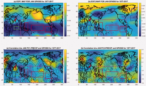
Table 7. Correlation matrix between PCs of GPH (G1, G2, G3) and PCs of Region1 precipitation (PC1, PC2 and PC3).

GPH-principal components	R1JANP-PC1		R1JANP-PC2		R1JANP-PC3
	Corrl. coeff.	p-value	Corrl. coeff.	p-value	Corrl. coeff.	p-value
G1	0.3532	2.35%	0.1062	50.88%	−0.2619	9.81%
G2	−0.2594	10.15%	0.1453	36.46 %	−0.1598	31.83%
G3	−0.0693	66.88%	−0.1881	23.90%	0.2259	15.56%

Bold figures indicate significant correlation at 10% confidence.

Table 8. Correlation between PCs of GPH (G1, G2, G3) and climate indices.

Indices	G1		G2
	Corrl. coeff.	p-value	Corrl. coeff.	p-value
NAO	−0.1475	0.3576	0.2284	0.1508
AO	−0.0369	0.8188	0.1591	0.3203
AMO	−0.4251	0.0056	−0.0742	0.6449
DMI	−0.1188	0.4595	−0.2821	0.0739
EQWIN	0.3237	0.0390	0.0147	0.9272
ENSO-MEI	0.0650	0.6865	0.0366	0.8204
EMI-MODOKI	−0.2029	0.2033	0.0631	0.6953
PDO	−0.1510	0.3461	−0.1802	0.2595

Bold and highlighted figures indicate significant correlation at 20% confidence.

3.4.6. Relationship of Region1 precipitation with surface wind anomalies for January

Figure 11 below shows the distribution of correlation coefficient between PCs (1, 2 and 3) and standardized Zonal Winds at Surface (ZW-Surface) for the month of January. As mentioned above, EQWIN being highly correlated to EQUINOO, correlations of PCs with OLR is calculated to identify the influence of EQWIN index easily (Fig. 12). In tropical Indian Ocean at WEIO and EEIO regions, OLR anomalies are significantly correlated with the PC1, PC3 of Region1 precipitation which is indicative of correlation with surface zonal winds whereas association with PC-2 remains insignificant. This surface zonal wind anomaly is indicative of EQWIN significant positive correlation with R1JANP. (For EQWIN index the negative anomaly of OLR is to be multiplied with −1).

Fig. 11. PCs of standardized ZW-Surface for January over 1977–2017. (a) PC1 shows strong patterns of EQWIN. (b) PC2 shows weak pattern of EQWIN whereas (c) PC3 shows weak pattern of EQWIN. Black boxes show WEIO and EEIO region whereas green box shows CEIO region in Indian Ocean. Red boxes show ENSO-MODOKI regions whereas magenta box shows ENSO-MEI region in Pacific Ocean. Blue boxes show NAO region in Atlantic Ocean.

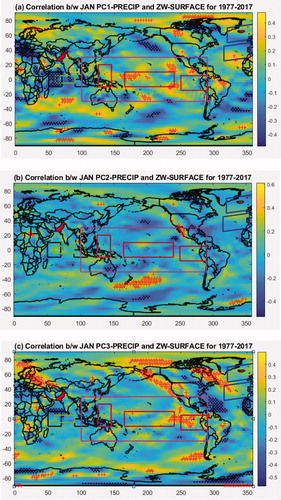
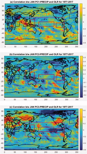
Fig. 12. EOFs of standardized OLR for January over 1977–2017. (a) EOF1 shows strong patterns of EQWIN. (b) EOF2 shows weak pattern of EQWIN whereas (c) EOF3 shows patterns of EQWIN. Black boxes show WEIO and EEIO region whereas green Box shows CEIO region in Indian Ocean. Red boxes show ENSO-MODOKI regions whereas magenta box shows ENSO-MEI region in Pacific Ocean. Blue boxes show NAO region in Atlantic Ocean.

3.4.7. Time-lag relationship of PCs with climate indices for January

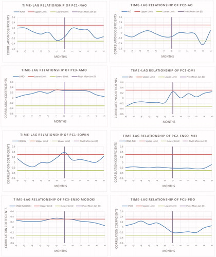
Figure 13 shows the time-lag relationship of correlation coefficient of PCs with the climate indices. As mentioned earlier, three PCs of Region1 precipitation are considered. Time-lag relationship of only those PC-Climate Index relationship is considered which is most significant. For example, out of the three relationships between PCs and NAO; only PC1-NAO is most significant which is shown in Table 6. Time-lag relationship indicates that except NOA all the other climate indices (AO, AMO, DMI, EQWIN, ENSO-MEI, EMI-MODOKI and PDO) are at their maximum significance level with the respective principal mode (PC) preceding to the month of January. NAO attains its maximum negative significance in December of the year preceding the month of January. Time-lag relationship also shows that NAO, AO, ENSO-MEI and PDO are negatively correlated whereas AMO, DMI, EQWIN and ENSO-MODOKI are positively correlated with their respective principal modes of precipitation.

Fig. 13. Time-lag correlation coefficient between most significant PCs and Climate Indices. January is considered as the pivot month with a value “0” represented by a vertical line whereas negative/positive values along x-axis (Months) indicates preceding/following months from January. Upper and lower limit represents the significance level of 5%.

3.4.8. Results of analyses for January

The results obtained from all the above analyses are summarized in the Table 9 below along with the comparison with the previously obtained results of correlation and Partial Mann-Kendall analyses. Thus, from the analysis, it can be concluded that influence of NAO and AO on Region1 precipitation is insignificant (weak). Since none of the previous studies were focused on Baluchistan as such there is not much literature available to support the argument that NAO mode enhances (reduces) the precipitation in Baluchistan. However, Ahmed et al. (2015) found out that the positive (negative) NAO mode strengthens (weakens) winter spring precipitation in Pakistan similarly Athar et al. (2015) found out that NAO shows a correlation with Baluchistan without mentioning whether the correlation is positive or negative. Therefore, it can be stated that NAO and AO have weak influence on the January precipitation in Baluchistan. The influence of AMO, DMI, ENSO-MEI and PDO is significant up to 20% confidence (may be considered as moderate). Lastly, the influence of EQWIN and EMI-MODOKI is significant up to 5% confidence (may be considered as strong).

Table 9. Summary of analysis results for Region1 precipitation and climate indices for January.

Indices/ Teleconnection	Partial Mann-Kendall	Correlation b/w PCs and Climate Indices	EOF analysis	Correlation b/w PCs and anomalies of
				SST	Atmospheric circulation	Zonal winds/OLR
NAO	Weak	Insignificant	Weak	Weak	Moderate	–
AO	Weak	Insignificant	Moderate to Weak	–	Weak	–
AMO	Weak	Significant at 7.9%	Moderate	Moderate	–	–
DMI	Weak	Significant at 12.4%	Moderate	Moderate	–	–
EQWIN	Strong to Moderate	Significant at 1.5 %	Strong	–	–	Strong
ENSO-MEI	Moderate to Weak	Significant at 16.5 %	Moderate	Weak	–	–
EMI-MODOKI	Strong	Significant at 4.8 %	Strong	Strong	–	–
PDO	Weak	Significant at 20.5 %	Moderate	Moderate to Strong	–	–

Where ‘–’ means not applicable.

3.5. Linkages of June precipitation variability with climatic indices

3.5.1. Modes of Region1 precipitation for the month of June

PCA is performed on the R1JUNP for the period 1977 to 2017. First three (3) EOFs explain 90.82% variation, capable enough to explain the precipitation variability in Region1 (Table 10) and these three (3) PCs are then used to perform the correlation analysis with climate indices. The correlation between time series of PCs and R1JUNP is shown in Table 10. The selected PCs are shown as highlighted.

3.5.2. Correlation of region1 precipitation with climate indices for June

In order to find out the association of R1JUNP with climate indices, correlation is performed between time series of Region1 precipitation PC (R1JUNP-PCs) and the climate indices for the respective month of June. The results are presented in Table 11. Large scale teleconnection circulation patterns NAO is positively correlated to PC2 at 7.95% confidence. AO is positively correlated to PC2 at 18.30% confidence. Atlantic Multi Decadal Oscillation index (AMO) is negatively correlated to PC3 at 13.42% confidence. Indian Ocean Dipole mode index DMI is positively correlated to PC1 at 13.89% confidence. Indian Ocean Circulation pattern defined by EQWIN is positively correlated to PC1 at 21.19%. Large scale Teleconnection pattern ENSO-MEI is positively correlated to PC3 at 6.02% confidence. ENSO-MODOKI Index (EMI-MODOKI) is negatively correlated to PC3 at 2.55% confidence. Pacific Ocean decadal oscillation (PDO) is negatively correlated to PC2 at 4.26% confidence.

Table 11. Correlation between R1JANP-PCs and climate indices.

Indices	R1JUNP-PC1		R1JUNP-PC2		R1JUNP-PC3
	Corrl. coeff.	p-value	Corrl. coeff.	p-value	Corrl. coeff.	p-value
NAO	−0.2530	0.1105	−0.0091	0.9549	−0.0521	0.7463
AO	−0.1120	0.4858	0.0179	0.9114	−0.0406	0.8011
AMO	−0.0625	0.6978	−0.0371	0.8178	0.0629	0.6958
DMI	0.1503	0.3483	0.1437	0.3699	−0.0520	0.7470
EQWIN	0.4397	0.0040*	−0.0111	0.9449	−0.2191	0.1687
ENSO-MEI	0.0257	0.8732	0.0970	0.5464	−0.1468	0.3597
EMI-MODOKI	0.1170	0.4662	−0.0295	0.8549	0.1264	0.4309
PDO	0.1338	0.4044	−0.3139	0.0457*	−0.1096	0.4951

Bold with asterick figures indicate significant correlation up to 8% confidence whereas bold figures indicate correlation up to 20% confidence.

3.5.3. Leading modes of teleconnection patterns for the month of June

EOF analysis is performed on SST, SLP and ZW-surface for the month of June also. The uncertainty estimates of June eigenvalues spectrum of covariance matrix of SST and SLP are calculated and is used for selecting leading modes of EOFs. Two eigenvalues of SST and four eigenvalues of SLP are well distinguishable from the rest of the spectrum as shown in Fig. 14a,b. Therefore, three leading modes for each of teleconnection patterns are considered for the analysis.

Fig. 14. (a) Eigenvalue spectrum (%) of the covariance matrix of June SST. The vertical bar shows uncertainty estimates based on North et al. (1982) rule of thumb. The leading 25 eigenvalues out of 41 are shown. (b) Eigenvalue spectrum (%) of the covariance matrix of June SLP. The vertical bar shows uncertainty estimates based on North et al. (1982) rule of thumb. The leading 25 eigenvalues out of 41 are shown.

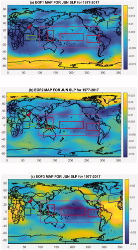
Three leading modes EOF1(15%), EOF2(12%) and EOF3(7%) of SST explained about 34% cumulative variability and shows the teleconnection patterns of ENSO, EMI-MODOKI (warm center flanked by cold sides: cold center flanked by warm sides) in Central Pacific Ocean, AMO in North Atlantic Ocean, NAO (associated SST pattern) in North Atlantic Ocean, DMI pattern (though weak) in Indian Ocean. Leading modes of SST are shown in Fig. 15a–c, respectively. Fig. 16a–c shows three leading modes of SLP. EOF1 (17%), EOF2 (11%) and EOF3(9%) of SLP explained about 37% cumulative variability and shows the patterns of ENSO, NAO and AO (though not very distinguishable).

Fig. 15. EOFs of standardized SST for June over 1977–2017. (a) EOF1 shows the Pattern of EMI-MODOKI in central Pacific Ocean though weak in one of the flank and AMO in North Atlantic Ocean. (b) EOF2 shows the patterns of NAO (associated SST pattern; though weak) in North Atlantic Ocean, ENSO-MEI in central Pacific and PDO in North Pacific. (c) EOF3 shows weak patterns of DMI, EMI-MODOKI and NAO (associated SST pattern). Black boxes show WEIO and EEIO region whereas green Box shows CEIO region in Indian Ocean. Red boxes show ENSO-MODOKI regions whereas magenta box shows ENSO-MEI region in Pacific Ocean. Blue boxes show NAO region in Atlantic Ocean.

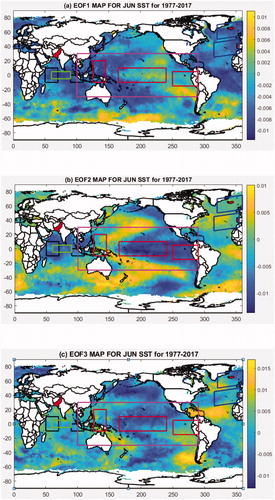
Fig. 16. EOFs of standardized SLP for June over 1977–2017. (a) EOF1 shows the Pattern of NAO though not very distinguished. (b) EOF2 shows the pattern of NAO. (c) EOF3 shows patterns of ENSO-MEI and AO though not very distinguished. Black boxes show WEIO and EEIO region whereas green box shows CEIO region in Indian Ocean. Red boxes show ENSO-MODOKI regions whereas magenta box shows ENSO-MEI region in Pacific Ocean. Blue boxes show NAO region in Atlantic Ocean.

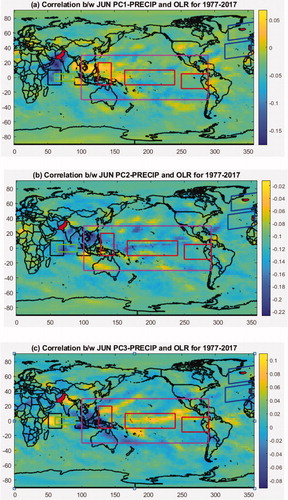
Leading modes of ZW-Surface are shown in Fig. 17a–c, respectively. EOF1(9%), EOF2(7%) and EOF3(6%) of ZW-Surface explained about 23% cumulative variability. As mentioned above, EQWIN is highly correlated with the difference of OLR in EEIO and WEIO regions therefore the occurrence of EQWIN can easily be detected by identifying the enhanced/suppressed convection (cloudiness) in WEIO/EEIO region. EOFs of OLR are shown in Fig. 18a–c. EOF1 and EOF2 depicts weak pattern whereas EOF3 shows moderate pattern of EQWIN.

Fig. 17. EOFs of standardized ZW-surface for June over 1977–2017. (a) EOF1 shows weak patterns of EQWIN. (b) EOF2 shows weak pattern of EQWIN whereas (c) EOF3 shows patterns of EQWIN. Black boxes show WEIO and EEIO region whereas green box shows CEIO region in Indian Ocean. Red boxes show ENSO-MODOKI regions whereas magenta box shows ENSO-MEI region in Pacific Ocean. Blue boxes show NAO region in Atlantic Ocean.

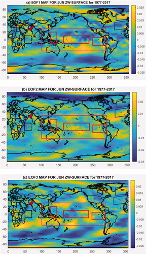
Fig. 18. EOFs of standardized OLR for June over 1977–2017. (a) EOF1 shows weak patterns of EQUINOO. (b) EOF2 shows weak pattern of EQUINOO whereas (c) EOF3 shows moderate patterns of EQUINOO. Black boxes show WEIO and EEIO region whereas green box shows CEIO region in Indian Ocean. Red boxes show ENSO-MODOKI regions whereas magenta box shows ENSO-MEI region in Pacific Ocean. Blue boxes show NAO region in Atlantic Ocean.

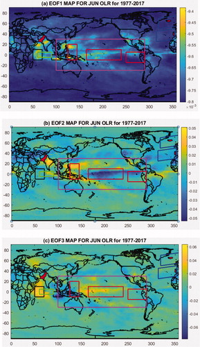
From the EOF analysis as above, it is clear that patterns of NAO (weak), AO (None), AMO (moderate), DMI (weak), EQWIN (strong), ENSO-MEI (moderate to strong), EMI-MODOKI (weak) and PDO (moderate to strong) are found in the three leading modes of June.

3.5.4. Relationship of region1 precipitation with SST anomalies for June

Figure 19 below shows the distribution of correlation coefficient between PCs (1, 2 and 3) and standardized SST for the month of June. In tropical areas, PC-1 and PC-3 are negatively correlated with central-Eastern pacific whereas they are positively correlated with western pacific (Fig. 19a,c). This surface SST anomaly is indicative of linkages of precipitation with ENSO-MEI, but the correlation is mostly insignificant with some significant areas and may be considered as weak which is in line with the findings in Table 6. Figure 19b show positive correlation in the central area for EMI-MODOKI and negative correlation in flank areas marked by red boxes but with weak strength, which is indicative of weak linkages of PC2 with the EMI-MODOKI Index. At mid and high latitudes, PC1 and PC2 are negatively and positively correlated with SSTs analogous to PDO index (Fig. 19a,b). The correlation of PC1 with PDO may be considered as moderate but it may be considered as strong with PC2. PC3 shows correlation analogous to PDO pattern but not very distinguished.

Fig. 19. Correlation between PCs of Region1 precipitation and standardized SST for June over 1977–2017. (a) PC1 shows weak correlation with NAO (associated SST pattern) and ENSO-MEI whereas moderate correlation with PDO. (b) PC2 shows weak correlation with EMI-MODOKI and string correlation with PDO. (c) PC3 shows weak correlation with DMI and ENSO-MEI but moderate correlation with AMO. Black boxes show WEIO and EEIO region whereas green box shows CEIO region in Indian Ocean. Red boxes show ENSO-MODOKI regions whereas magenta box shows ENSO-MEI region in Pacific Ocean. Blue boxes show NAO region in Atlantic Ocean.

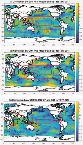
In tropical Indian ocean, PC1 does not show any distinguishable positive/negative correlations in WEIO/EEIO region. Both PC2 and PC3 are positively/negatively correlated with SST in WEIO/EEIO but the correlation is weak. These SST anomalies over WEIO/EEIO region is indicative of linkages with DMI but the correlation appears weak with some significant positive correlations.

In Northern Atlantic Ocean, PC1 (Fig. 19a) is correlated with SST anomalies analogous to the NAO associated SST pattern, thus indictive of association with NAO. PC2 show no correlation pattern similar to NAO but the correlation is weak. Figure 19c shows moderate positive correlation with SST in Northern Atlantic which is indicative of AMO linkage with PC3.

3.5.5. Relationship of Region1 precipitation with atmospheric circulation anomalies for June

The relationship of Region1 precipitation with atmospheric circulations is studied by conducting the correlation analysis between PCs and atmospheric circulations SLP, GPH500. Figure 20 below shows the distribution of correlation coefficient between PCs (1, 2, 3) and standardized SLP for the month of June. In tropical region, the pacific warm pool shows some significant correlation with Region1 precipitation. Responding to PC3, the Eastern-Central tropical region shows negative correlation with SLP whereas western tropical region shows positive correlation analogous to ENSO pattern. Similarly, responding to PC1 the center tropical region shows negative correlation with SLP and positive correlation in flank areas marked by red boxes. This surface SLP anomaly is indicative of linkages with ENSO-MODOKI, but the correlation is mostly insignificant with some significant areas. Responding to PC2, central Indian and Pacific Ocean shows negative correlation with some significant correlated areas.

Fig. 20. Correlation between PCs of Region1 precipitation and standardized SLP for June over 1977–2017. (a) PC1 with SLP. (b) PC2 with SLP. (c) PC3 with SLP. Black boxes show WEIO and EEIO regions. Black boxes show WEIO and EEIO region whereas green box shows CEIO region in Indian Ocean. Red boxes show ENSO-MODOKI regions whereas magenta box shows ENSO-MEI region in Pacific Ocean. Blue boxes show NAO region in Atlantic Ocean. Red ‘+’ and Black ‘.’ stipples show significant positive and negative correlation at 5% confidence, respectively.

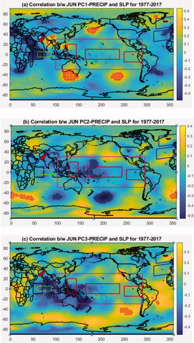
In Indian ocean, responding to SLP, PC1 and PC3 show significant negative correlation while PC-2 shows weak negative/positive correlation at WEIO/EEIO regions to DMI Index.

In Northern Atlantic Ocean, high pressure anomaly is present over Iceland whereas significant low-pressure anomaly is present over Azores in response to correlation of PC1 with SLP. This surface SLP anomaly is indicative of strong (-) NAO pattern. Responding to SLP, PC2 is positively correlated with Azores region and negatively correlated with Iceland region but the correlations remain insignificant (weak). This SLP anomaly is indicative of + NAO mode. PC3 again shows positive correlation with Azores and negative correlation with Iceland with insignificant correlations (weak). Responding to SLP, PC1, PC2 and PC3 does not show any significant correlation analogous to AO pattern although some positive and negative correlations are present in Arctic region.

In order to understand the linkages of the observed signals of teleconnection including EMI-MODOKI, ENSO-MEI in Pacific Ocean, DMI in Indian Ocean, NAO, AO in Atlantic Ocean with Region1 precipitation through atmospheric circulations, the correlation is performed between of PCs (1, 2, 3) with GPH500 as shown in Fig. 21. In response to correlations of PC1 with SLP and GPH500, Fig. 20a shows positive surface pressure at region1 whereas Fig. 21a depicts negative pressure anomaly (at GPH500) which is indicative of anti-cyclonic conditions with reduced precipitation. Negative/positive SLP anomaly at Azores/Iceland with its counterpart negative/positive anomaly at 500 hpa extending all the way to Mediterranean and Middle East Region which is indicative of linkages with NAO. Further in tropical pacific region positive/negative/positive SLP anomaly with its counterpart negative/positive/negative GPH500 anomaly in EMI-MODOKI regions are not very supportive for teleconnection pattern of EMI-MODOKI Index. For PC2 correlations with responding SLP and GPH500, Figs. 8b and 9b shows that the pressure conditions at surface are supportive of its counterpart pressure conditions at mid altitude. Similarly, cyclonic condition exists in Indian Ocean represented by negative SLP anomaly and positive mid altitude anomaly at 500 hpa which is indicative of enhance precipitation. Lastly, for PC3 correlations with SLP and GPH500, Figs. 8c and 9c shows anti-cyclonic conditions over Region1 in response to anti-cyclonic condition at SLP and cyclonic condition at mid heights over tropical Indo-pacific region and north Atlantic region which is indicative of reduced precipitation.

Fig. 21. Correlation between PCs of Region1 precipitation and standardized GPH500 for June over 1977–2017. (a) PC1 with GPH500. (b) PC2 with GPH500. (c) PC3 with GPH500. Black boxes show WEIO and EEIO regions. Black boxes show WEIO and EEIO region whereas green box shows CEIO region in Indian Ocean. Red boxes show ENSO-MODOKI regions whereas magenta box shows ENSO-MEI region in Pacific Ocean. Blue boxes show NAO region in Atlantic Ocean. Red ‘+’ and Black ‘.’ stipples show significant positive and negative correlation at 5% confidence, respectively.

To ascertain the linkages of atmospheric circulations with Region1 precipitation, EOF modes of GPH500 are calculated. The target area is 30S − 90 N and 0 − 360 where the teleconnection pattern under consideration are shaped. The corresponding time series of the three leading modes (G1, G2, G3) which explains 52% combined variability are extracted. The correlation matrix between G1, G2, G3 with PCs of Region1 precipitation (PC1, PC2, PC3) is shown in Table 12. The matrix is formulated to determine the PCs of GPH500 which have significant influence on the Region1 precipitation through teleconnection via atmospheric circulations. Table 12 indicates that G1 and G2 have significant correlations with Region1 precipitation PC3 only and therefore are considered for further analysis. The leading EOF modes (EOF1, EOF2) and the correlation of PCs of Region1 precipitation (PC1, PC2) is shown in Fig. 22. The correlation analysis is performed between the G1, G2 and climate indices to determine the influencing indices of Region1 precipitation. The results are shown in Table 13 which indicates that Region1 precipitation is linked to AMO, EQWIN and EMI-MODOKI through atmospheric circulations.

Fig. 22. EOF modes of standardized GPH at 500 hpa in June and correlation with PCs of Region1 precipitation. (a) EOF1 mode of GPH500. (b) EOF2 mode of GPH500. (c) Correlation between PC1 with GPH500. (d) Correlation between PC2 with GPH500. Black boxes show WEIO and EEIO regions. Red boxes show ENSO-MODOKI Regions and Magenta box shows ENSO-MEI Region. Blue boxes show NAO region. Red ‘+’ and Black ‘.’ stipples show significant positive and negative correlation at 5% confidence, respectively.

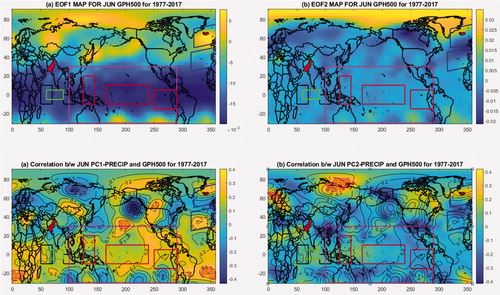
Table 12. Correlation matrix of p-value between PCs of GPH (G1, G2, G3) and PCs of Region1 precipitation (PC1, PC2 and PC3).

GPH-principal components	R1JUNP-PC1		R1JUNP-PC2		R1JUNP-PC3
	Corrl. coeff.	p-value	Corrl. coeff.	p-value	Corrl. coeff.	p-value
G1	0.0106	0.9476	−0.3545	0.0230	0.2023	0.2047
G2	0.2456	0.1217	−0.3343	0.0327	0.0941	0.5585
G3	−0.1356	0.3979	0.1822	0.2543	−0.1103	0.4925

Bold figures indicate significant correlation at 10% confidence.

Table 13. Correlation between PCs of GPH (G1, G2, G3) and climate indices.

Indices	G1		G2
	Corrl. coeff.	p-value	Corrl. coeff.	p-value
NAO	0.0926	0.5648	0.0165	0.9184
AO	0.0586	0.7160	0.0282	0.8612
AMO	−0.2212	0.1646	−0.0865	0.5908
DMI	−0.0652	0.6857	−0.0676	0.6745
EQWIN	0.2216	0.1638	0.2609	0.0995
ENSO-MEI	−0.0531	0.7416	−0.1762	0.2704
EMI-MODOKI	−0.2356	0.1382	0.0055	0.9725
PDO	0.1245	0.4379	−0.0262	0.8706

Bold figures indicate significant correlation at 20% confidence.

3.5.6. Relationship of Region1 precipitation with surface wind anomalies for June

Figure 23 below shows the distribution of correlation coefficient between PCs (1, 2 and 3) and standardized Zonal Winds at Surface (ZW-Surface) for the month of June. As mentioned above, EQWIN being highly correlated to EQUINOO, correlations of PCs with OLR is calculated to identify the influence of EQWIN index easily (Fig. 24). In tropical Indian Ocean at WEIO and EEIO regions, OLR anomalies are significantly correlated with the PC1, PC3 of Region1 precipitation which is indicative of correlation with surface zonal winds whereas association with PC-2 remains insignificant and weak. This surface zonal wind anomaly is indicative of EQWIN significant positive correlation with R1JUNP. (For EQWIN index the negative anomaly is to be multiplied with −1).

Fig. 23. EOFs of standardized ZW-surface for June over 1977–2017. (a) EOF1 shows strong patterns of EQWIN. (b) EOF2 shows weak pattern of EQWIN whereas (c) EOF3 shows strong pattern of EQWIN. Blue box shows WEIO region and red box shows EEIO region. Black boxes show WEIO and EEIO region whereas green box shows CEIO region in Indian Ocean. Red boxes show ENSO-MODOKI regions whereas magenta box shows ENSO-MEI region in Pacific Ocean. Blue boxes show NAO region in Atlantic Ocean. Red ‘+’ and Black ‘.’ stipples show significant negative and positive correlation at 5% confidence respectively.

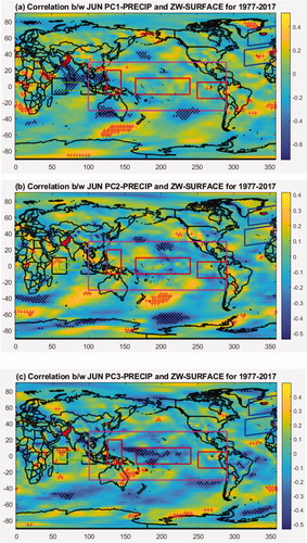
Fig. 24. EOFs of standardized ZW-surface for June over 1977–2017. (a) EOF1 shows moderate patterns of EQUINOO. (b) EOF2 shows weak pattern of EQUINOO whereas (c) EOF3 shows moderate pattern of EQUINOO. Blue box shows WEIO region and red box shows EEIO region. Black boxes show WEIO and EEIO region whereas green box shows CEIO region in Indian Ocean. Red boxes show ENSO-MODOKI regions whereas magenta box shows ENSO-MEI region in Pacific Ocean. Blue boxes show NAO region in Atlantic Ocean. Red ‘+’ and Black ‘.’ stipples show significant negative and positive correlation at 5% confidence respectively.

3.5.7. Time-lag relationship of PCs with climate indices for June

Figure 25 shows the time-lag relationship of correlation coefficient of PCs with the climate indices. As mentioned earlier, three PCs of Region1 precipitation are considered. Time-lag relationship of only those PC-Climate Index relationship is considered which is most significant. Time-lag relationship indicates the climate indices NAO, AO, EQWIN and PDO are at their maximum significance level with the respective principal mode (PC) preceding to the month of June. AMO attains its maximum negative significance in January of the year preceding the month of June whereas DMI, ENSO-MEI and ENSO-MODOKI attains their maximum significance in preceding month of May. Time-lag relationship also shows that AMO, DMI, EQWIN and ENSO-MODOKI are positively correlated whereas NAO, AO, ENSO-MEI and PDO are negatively correlated with their respective principal modes of precipitation.

Fig. 25. Time-lag correlation coefficient between most significant PCs and Climate Indices. June is considered as the pivot month with a value “0” represented by a vertical line whereas negative/positive values along x-axis (Months) indicates preceding/following months from June. Upper and lower limit represents the significance level of 5%.

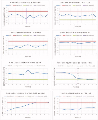
Fig. C1. (a) Spatial distribution – average Region1 precipitation January. (b) Spatial distribution – average Region1 precipitation June.

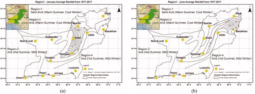
Fig. C2. (a) Spatial dsistribution of EOF1 of January. (b) Temporal variation of PC-1 of January.

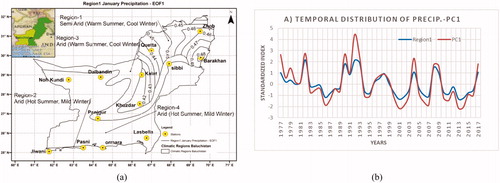
Fig. C3. (a) Spatial distribution of EOF-2 of January. (b) Temporal variation of PC-2 of January.

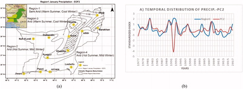
Fig. C4. (a) Spatial distribution of EOF-3 of January. (b) Temporal variation of PC-3 of January.

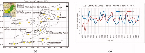
Fig. C5. (a) Spatial distribution of EOF-1 of June. (b) Temporal variation of PC-1 of June.

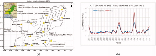
Fig. C6. (a) Spatial distribution of EOF-2 of June. (b) Temporal variation of PC-2 of June.

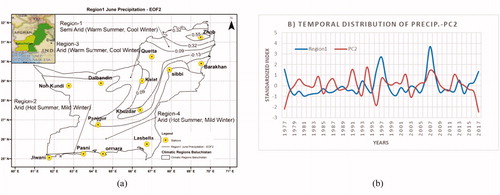
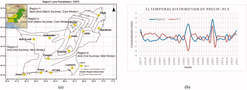
Fig. C7. (a) Spatial distribution of EOF-3 of June. (b) Temporal variation of PC-3 of June. Refer to Fig. C2b the precipitation index is −0.18 in the year 1983. The EMI-Modoki and NAO index are unusually at −2.98 and +4.824 respectively in January 1983 which may be attributed to the post volcanic eruption of Mount El Chichon-Mexico in March 1982. Similarly, refer to Fig. C5b, the negative precipitation anomaly as is observed in the year June 1982 and June 1991 following the volcanic eruption of Mount El Chichon-Mexico in March 1982 and Mount Pinatubo-Phillipines in June 1991 may be because of variation in climate patterns unfavorable to precipitation due to post volcanic eruption changes in EMI-Modoki and EQWIN indices (Dogar et al., 2017; Dogar, 2018; Dogar and Sato, 2019).

3.5.8. Results of analyses for June

The results obtained from all the above analyses are summarized in the Table 14 below along with the comparison with the previously obtained results of correlation and Partial Mann-Kendall analyses. Thus, from the analyses, it can be concluded that influence of AO, DMI and EMI-MODOKI on Region1 precipitation is insignificant (weak). The influence of NAO, AMO and ENSO-MEI may be considered as moderate. Lastly the influence of EQWIN and PDO are significant up to 5% confidence (may be considered as strong). It is found that the Indian Summer Monsoon Rainfall (ISMR) is influenced by IOD (Ashok et al., 2001; Vishnu et al., 2019). As explained in para 2.2.2, DMI and EQWIN are the oceanic and atmospheric circulation indices that describes Indian Ocean Dipole (IOD). In this study, EQWIN is found to be more correlated than DMI having moderate to strong influence on June precipitation.

Table 14. Summary of analysis results for Region1 precipitation and climate indices for June.

Indices/ Teleconnection	Partial Mann-Kendall	Correlation b/w PC1 and climate indices	EOF analysis	Correlation b/w PCs and anomalies of
				SST	atmospheric circulation	Zonal winds and OLR
NAO	Weak	Significant at 11.05%	Weak	Weak	Moderate	–
AO	Weak	Insignificant	Weak	–	–	–
AMO	Weak	Insignificant	moderate	Moderate	–	–
DMI	Weak	Insignificant	Weak	Weak	Weak	–
EQWIN	Strong	Significant at 0.4 %	Strong	Moderate	–	Moderate to Strong
ENSO-MEI	Weak	Insignificant	Strong	Weak	–	–
EMI-MODOKI	Strong	Insignificant	Weak	Weak	Weak	–
PDO	Weak	Significant at 4.57 %	Strong	Strong	–	–

Where ‘–’ means not applicable.

4. Conclusion

Baluchistan receives its greater portion of the rainfall in winter and spring months. Decreasing Trends in precipitation are observed in the months of January in Region1, when the time series data are analyzed from 1977 to 2017 through Mann- Kendall Test, which confirms that the Baluchistan is receiving lesser rainfall since the past few decades. The change in trends under the influence of climatic Indices is determined through PMK for the month of January and June in Region1. EQWIN, ENSO-MEI and EMI-MODOKI shows moderate to strong influence on precipitation.

It is determined through correlation of time series of Region1 Precipitation (PCCs) and climate indices that NAO, AMO, EQWIN, EMI-MODOKI and PDO are influencing the precipitation in January and explain the maximum variability of the precipitation in January. EQWIN, EMI-MODOKI and AMO are positively correlated with principle modes of January precipitation up to 8% significance whereas PDO and NAO are negatively correlated with the January precipitation but are insignificant (their significance is in between 20% to 35%) and thus can be ignored. NAO was found out to be favorable for winter and spring precipitation over Pakistan as per previous studies, but its effect is determined as insignificant for January precipitation in the Region1 of Baluchistan. AMO is in its warmer phase since 1997 and it is observed from the time series that the strength of NAO and AO is weakened during this time period of warm AMO phase. The decreasing trend may be due to the weakening of NAO strength during past few decades which is negatively affecting the January precipitation.

Slightly increasing trends are found in June precipitation, when the time series data are analyzed from 1977 to 2017 through Mann-Kendall Test. NAO, AMO, EQWIN, ENSO-MEI and PDO are found to be influencing the June precipitation as determined through correlation analysis between PCs and climate indices. AMO may be considered as positively correlated whereas NAO and ENSO-MEI may be considered as negatively correlated, but their strengths are insignificant to weak. PDO is negatively correlated to the principle modes of region1 precipitation at 5% significance which means that the negative phase of PDO is favorable for June precipitation; whereas EQWIN is positively correlated with June precipitation at 1% significance which means that positive phase is favorable for June precipitation. It is observed that the average precipitation in June 2007 was high (86.4 mm). During this year PDO (0.09) and AMO (−0.08) were neutral, NAO (−3.339), ENSO-MEI (−0.215) were negative whereas EQWIN (0.66) was positive which confirms the correlation findings as above and accounts for the slight increasing trend in the June precipitation. The influencing climatic indices for the months of January and June over the Region1 of Baluchistan as identified through EOF maps, PCA and correlation analyses can be used as the possible predictors of precipitation for further studies.

Acknowledgements

The authors would like to thank the editor anonymous reviewers for their valuable comments and suggestions to improve the quality of the manuscript. The authors would also like to thank PMD for providing the station data, ESRL and NCEP of NOAA (USA) for providing the circulation indices’ data.

Disclosure statement

The authors declare no conflict of interest.

Appendix A

Table A2. Influence of NAO on precipitation trends.

Months	Stations	Mann-Kendall			Partial Mann-Kendall with NAO as covariate			Change in MK-statistics due to NAO as Covariate	Influence type
		p-value	MK-statistic	Trend type	p-value	PMK-statistic	Trend type
January	Barakhan	0.0462	−177	Decreasing	0.048	−174.1	Decreasing	1.64%	Weak
	Quetta	0.0119	−224	Decreasing	0.0121	−223.4	Decreasing	0.27%	Weak
	Zhob	0.0239	−201	Decreasing	0.0245	−196.8	Decreasing	2.09%	Weak
June	Barakhan	0.0493	175	Increasing	0.0576	168.8	Increasing	3.54%	Weak

Table A3. Influence of AO on precipitation trends.

Months	Stations	Mann-Kendall			Partial Mann-Kendall with AO as Covariate			Change in MK-statistics due to AO as covariate	Influence type
		p-value	MK-statistic	Trend type	p-value	PMK-statistic	Trend type
January	Barakhan	0.0462	−177	Decreasing	0.0397	−179	Decreasing	1.13%	Weak
	Quetta	0.0119	−224	Decreasing	0.0113	−225.4	Decreasing	0.63%	Weak
	Zhob	0.0239	−201	Decreasing	0.0268	−196.1	Decreasing	2.44%	Weak
June	Barakhan	0.0493	175	Increasing	0.0457	176.5	Increasing	0.86%	Weak

Table A4. Influence of AMO on precipitation trends.

Months	Stations	Mann-Kendall			Partial Mann-Kendall with AO as Covariate			Change in MK-statistics due to AO as covariate	Influence Type
		p-value	MK-statistic	Trend type	p-value	PMK-statistic	Trend Type
January	Barakhan	0.0462	−177	Decreasing	0.0397	−179	Decreasing	1.13%	Weak
	Quetta	0.0119	−224	Decreasing	0.0113	−225.4	Decreasing	0.63%	Weak
	Zhob	0.0239	−201	Decreasing	0.0268	−196.1	Decreasing	2.44%	Weak
June	Barakhan	0.0493	175	Increasing	0.0457	176.5	Increasing	0.86%	Weak

Table A5. Influence of IOD-DMI on precipitation trends.

Months	Stations	Mann-Kendall			Partial Mann-Kendall with IOD as Covariate			Change in MK-statistics due to IOD as covariate	Influence type
		p-value	MK-statistic	Trend type	p-value	PMK-statistic	Trend type
January	Barakhan	0.0462	−177	Decreasing	0.0338	−188	Decreasing	6.21%	Weak
	Quetta	0.0119	−224	Decreasing	0.0086	−233.4	Decreasing	4.20%	Weak
	Zhob	0.0239	−201	Decreasing	0.0124	−221	Decreasing	9.95%	Moderate
June	Barakhan	0.0493	175	Increasing	0.0485	175.6	Increasing	0.34%	Weak

Table A6. Influence of IOD-EQWIN on precipitation trends.

Months	Stations	Mann-Kendall			Partial Mann-Kendall with PDO as covariate			Change in MK-statistics due to PDO as covariate	Influence type
		p-value	MK-statistic	Trend type	p-value	PMK-statistic	Trend type
January	Barakhan	0.0462	−177	Decreasing	0.0325	−153	Decreasing	13.56%	Strong
	Quetta	0.0119	−224	Decreasing	0.021	−202.6	Decreasing	9.55%	Moderate
	Zhob	0.0239	−201	Decreasing	0.0521	−166.9	Decreasing	16.97%	Strong
June	Barakhan	0.0493	175	Increasing	0.008	210.9	Increasing	20.51%	Strong

Table A7. Influence of ENSO-MEI on precipitation trends.

Months	Stations	Mann-Kendall			Partial Mann-Kendall with ENSO-MEI as covariate			Change in MK-statistics due to ENSO-MEI as covariate	Influence type
		p-value	MK-statistic	Trend type	p-value	PMK-statistic	Trend type
January	Barakhan	0.0462	−177	Decreasing	0.0437	−182.5	Decreasing	3.11%	Weak
	Quetta	0.0119	−224	Decreasing	0.0161	−213	Decreasing	4.91%	Weak
	Zhob	0.0239	−201	Decreasing	0.0362	−183.7	Decreasing	8.61%	Moderate
June	Barakhan	0.0493	175	Increasing	0.041	181	Increasing	3.43%	Weak

Table A8. Influence of MODOKI on precipitation trends.

Months	Stations	Mann-Kendall			Partial Mann-Kendall with ENSO-MEI as Covariate			Change in MK-statistics due to ENSO-MEI as covariate	Influence type
		p-value	MK-statistic	Trend type	p-value	PMK-statistic	Trend type
January	Barakhan	0.0462	−177	Decreasing	0.1227	−135.3	Decreasing	23.56%	Strong
	Quetta	0.0119	−224	Decreasing	0.1036	−136.8	Decreasing	38.93%	Strong
	Zhob	0.0239	−201	Decreasing	0.1798	−112.4	Decreasing	44.08%	Strong
June	Barakhan	0.0493	175	Increasing	0.1076	140.9	Increasing	19.49%	Strong

Table A9. Influence of PDO on precipitation trends.

Months	Stations	Mann-Kendall			Partial Mann-Kendall with PDO as covariate			Change in MK-statistics due to PDO as covariate	Influence type
		p-value	MK-statistic	Trend type	p-value	PMK-statistic	Trend type
January	Barakhan	0.0462	−177	Decreasing	0.0325	−185.9	Decreasing	5.03%	Weak
	Quetta	0.0119	−224	Decreasing	0.0097	−228.8	Decreasing	2.14%	Weak
	Zhob	0.0239	−201	Decreasing	0.0219	−203.5	Decreasing	1.24%	Weak
June	Barakhan	0.0493	175	Increasing	0.0357	183.4	Increasing	4.80%	Weak

 

Appendix B

The relationship between the original time series A(x,y,t) in terms of B(x,y) and Principal Component P(t) is given by $$A\left(x,y,t\right)=\sum _{k=1}^N\left(\mathrm{P}\left(\mathrm{t}\right)+\mathrm{B}(\mathrm{x}.\mathrm{y})\right)$$ where,

A(x,y,t) is the original time series as a function of time (t) and space (x,y). B(x,y) show the spatial structures (x,y) of the major factors that can account for the temporal variation of A. P(t) is the Principal Component that tells how the amplitude of each EOF varies with time.

Appendix C

References

- Aamir, E. and Hassan, I. 2018. Trend analysis in precipitation at individual and regional levels in Baluchistan. IOP Conf. Ser. Mater. Sci. Eng. 414, 012042. doi:10.1088/1757-899X/414/1/012042
- Abraham, A., Sajith, N. and Joseph, B. 2001. Will We Have a Wet Summer? Long-Term Rain Forecasting Using Soft Computing Models: Modeling and Simulation. Publication of the Society for Computer Simulation International, Prague, Czech Republic, pp. 1044–1048.
- Adnan, M., Khan, F., Rehman, N., Ali, S., Hassan, S. S. and co-authors. 2020. Variability and predictability of summer monsoon rainfall over Pakistan. Asia-Pac. J. Atmos. Sci. 1–9.
- Afzal, M., Haroon, M. A., Rana, A. S. and Imran, A. 2013. Influence of North Atlantic oscillations and Southern oscillations on winter precipitation of Northern Pakistan, Pakistan. Journal of Meteorology 9, 1–8.
- Ahmad, I., Ambreen, R., Sun, Z. and Deng, W. 2015. Winter-spring precipitation variability in Pakistan. AJCC 04, 115–139. doi:10.4236/ajcc.2015.41010
- Ahmad, I., Tang, D., Wang, T. F., Wang, M. and Wagan, B. 2015. Precipitation trends over time using Mann-Kendall and Spearman’s rho tests in Swat river basin, Pakistan. Adv. Meteorol. 2015, 1–15. doi:10.1155/2015/431860
- Ali, S., Khalid, B., Kiani, R. S., Babar, R., Nasir, S. and co-authors. 2020. Spatio-temporal variability of summer monsoon onset over Pakistan. Asia-Pacific J. Atmos. Sci. 56, 147–172. doi:10.1007/s13143-019-00130-z
- Arif, M., Tariq, M. A. and Nadem, F. 2004. Correlation between multivariate ENSO Index (MEI) and Pakistan’s summer rainfall. Pak. J. Meteorol. 1, 53–63.
- Ashok, K., Guan, Z. and Yamagata, T. 2001. Impact of the Indian Ocean dipole on the relationship between the Indian monsoon rainfall and ENSO. Geophys. Res. Lett. 28, 4499–4502. doi:10.1029/2001GL013294
- Ashraf, M. and Ashfaq A. S. 2017. Sustainable Groundwater Management in Balochistan. Pakistan Council of Research in Water Resources (PCRWR), Islamabad, Pakistan, p. 34.
- Ashraf, M. and Routray, J. K. 2015. Spatio-temporal characteristics of precipitation and drought in Balochistan Province. Nat. Hazards 77, 229–254. doi:10.1007/s11069-015-1593-1
- Ashraf, M., Routray, J. K. and Saeed, M. 2014. Determinants of farmers’ choice of coping and adaptation measures to the drought hazard in northwest Balochistan, Pakistan. Nat. Hazards 73, 1451–1473. doi:10.1007/s11069-014-1149-9
- Athar, H. 2015. Teleconnections and variability in observed rainfall over Saudi Arabia during 1978–2010. Atmos. Sci. Lett. 16, 373–379. doi:10.1002/asl2.570
- Available at: https://germanwatch.org/sites/germanwatch.org/files/20-2-01e%20Global, 20
- Bastiaanssen, W. G. M. and Ali, S. 2003. A new crop yield forecasting model based on satellite measurements applied across the Indus Basin, Pakistan. Agric. Ecosyst. Environ. 94, 321–340. doi:10.1016/S0167-8809(02)00034-8
- Burn, D. H. and Elnur, M. A. H. 2002. Detection of hydrologic trends and variability. J. Hydrol. 255, 107–122. doi:10.1016/S0022-1694(01)00514-5
- Butt, M. J. and Iqbal, M. F. 2009. Impact of climate variability on snow cover: a case study of northern Pakistan. Pak. J. Meteorol. 5, 53–63.
- Chaouche, K., Neppel, L., Dieulin, C., Pujol, N., Ladouche, B. and co-authors. 2010. Analyses of precipitation, temperature and evapotranspiration in a French Mediterranean region in the context of climate change. C. R. Geosci. 342, 234–243. doi:10.1016/j.crte.2010.02.001
- Chervenkov, H. and Slavov, K. 2019. Theil–Sen estimator vs. ordinary least squares—trend analysis for selected ETCCDI climate indices. C. R. Acad. Bulg. Sci. 72, 47–54.
- Dogar, M. M. 2018. Impact of tropical volcanic eruptions on Hadley circulation using a high-resolution AGCM. Current Science 114-1284. Available: http://dx.doi.org/10.18520/cs/v114/i06/1284-1294.
- Dogar, M. M., Kucharski, F. and Azharuddin, S. 2017. Study of the global and regional climatic impacts of ENSO magnitude using SPEEDY AGCM. J. Earth Syst. Sci. 126, 30. doi:10.1007/s12040-017-0804-4
- Dogar, M. M., Kucharski, F., Sato, T., Mehmood, S., Ali, S. and co-authors. 2019. Towards understanding the global and regional climatic impacts of Modoki magnitude. Global Planet. Change 172, 223–241. doi:10.1016/j.gloplacha.2018.10.004
- Dogar, M. M. and Sato, T. 2018. Analysis of climate trends and leading modes of climate variability for MENA region. J. Geophys. Res. Atmos. 123, 13,074–13,091. doi:10.1029/2018JD029003.
- Dogar, M. M. and Sato, T. 2019. Regional climate response of Middle Eastern, African, and South Asian monsoon regions to explosive volcanism and ENSO forcing. J. Geophys. Res. Atmos. 124, 7580–7598. doi:10.1029/2019JD030358
- Dogar, M. M., Stenchikov, G., Osipov, S., Wyman, B. and Zhao, M. 2017. Sensitivity of the regional climate in the Middle East and North Africa to volcanic perturbations. J. Geophys. Res. Atmos. 122, 7922–7948. doi:10.1002/2017JD026783
- Eckstein, D., Künzel, V., Schäfer, L. and Winges, M. 2019. Global Climate Risk Index 2020. Germanwatch. Available at: https://germanwatch.org/sites/germanwatch.org/files/20-2-01e%20Global,20,Bonn,Germany.
- Feldstein, S. B. and Franzke, C. L. 2017. Atmospheric teleconnection patterns. In Nonlinear and Stochastic Climate Dynamics, pp. 54–104, edited by Christen L. E. Franzke, Cambridge University press, CSIRO, Australia.
- Gadiwala, M. S. and Burke, F. 2019. Climate change and precipitation in Pakistan-a meteorological prospect. Int. J. Econ. Environ. Geol. 10–15.
- Global, C. 2020. China-Pakistan economic corridor: CPEC - CPIC. CPIC Global. Online at: https://www.cpicglobal.com/pakistan-overview/cpec/
- Gujarati, D. N. 2009. Basic Econometrics. Tata McGraw-Hill Education
- Hajani, E., Rahman, A. and Ishak, E. 2017. Trends in extreme rainfall in the state of New South Wales, Australia. Hydrol. Sci. J. 62, 2160–2174. doi:10.1080/02626667.2017.1368520
- Hanif, M., Khan, A. H. and Adnan, S. 2013. Latitudinal precipitation characteristics and trends in Pakistan. J. Hydrol. 492, 266–272. doi:10.1016/j.jhydrol.2013.03.040
- Hannachi, A., Jolliffe, I. T. and Stephenson, D. B. 2007. Empirical orthogonal functions and related techniques in atmospheric science: a review. Int. J. Climatol. 27, 1119–1152. doi:10.1002/joc.1499
- Haroon, M. A. and Rasul, G. 2009. Principal component analysis of summer rainfall and outgoing long-wave radiation over Pakistan. Pak. J. Meteorol. 5, 109–114.
- Hussain, M. S. and Lee, S. 2014. Long-term variability and changes of the precipitation regime in Pakistan. Asia-Pacific J. Atmos. Sci. 50, 271–282. doi:10.1007/s13143-014-0015-8
- IPCC. 2014. Climate change 2014: synthesis report. In Contribution of Working Groups I, II and III to the Fifth Assessment Report of the Intergovernmental Panel on Climate Change (eds. Core Writing Team, R. K. Pachauri and L. A. Meyer]. IPCC, Geneva, Switzerland, 151 pp.
- Iqbal, M. F. and Athar, H. 2018. Variability, trends, and teleconnections of observed precipitation over Pakistan. Theor. Appl. Climatol. 134, 613–632. doi:10.1007/s00704-017-2296-1
- Islamic Relief Pakistan. 2018. Drought Assessment Report. Islamic Relief Pakistan in Collaboration with PDMA Balochistan, p. 15. Available on: https://www.humanitarianresponse.info/en/operations/pakistan/document/islamic-relief-balochistan-drought-study-report-2018.
- Jamro, S., Dars, G. H., Ansari, K. and Krakauer, N. Y. 2019. Spatio-temporal variability of drought in Pakistan using standardized precipitation evapotranspiration index. Appl. Sci. 9, 4588. doi:10.3390/app9214588
- Kreft, S. and Eckstein, D. 2013. Global Climate Risk Index 2014. Who Suffers Most from Extreme Weather Events? Weather-Related Loss Events in 2012 and 1993 to 2012. German Watch Nord-Süd Initiative, Bonn, Germany.
- Krichak, S. O., Breitgand, J. S., Gualdi, S. and Feldstein, S. B. 2014. Teleconnection–extreme precipitation relationships over the Mediterranean region. Theor. Appl. Climatol. 117, 679–692. doi:10.1007/s00704-013-1036-4
- Latif, M. and Syed, F. S. 2016. Determination of summer monsoon onset and its related large-scale circulation characteristics over Pakistan. Theor. Appl. Climatol. 125, 509–520. doi:10.1007/s00704-015-1530-y
- Latif, M., Syed, F. S. and Hannachi, A. 2017. Rainfall trends in the South Asian summer monsoon and its related large-scale dynamics with focus over Pakistan. Clim. Dyn. 48, 3565–3581. doi:10.1007/s00382-016-3284-3
- Libiseller, C. 2004. Comparison of methods for normalization and trend testing of water quality data. In Proceedings of the Joint Meeting of the 6th International Symposium on Spatial Accuracy Assessment in Natural Resources and Environmental Sciences and The 15th Annual Conference of the International Environmetrics Society in Portland, Maine, USA.
- Libiseller, C. and Grimvall, A. 2002. Performance of partial Mann–Kendall tests for trend detection in the presence of covariates. Environmetrics: The Official Journal of the International Environmetrics Society 13, 71–84.
- Liu, D., Guo, S., Chen, X. and Shao, Q. 2012. Analysis of trends of annual and seasonal precipitation from 1956 to 2000 in Guangdong Province, China. Hydrol. Sci. J. 57, 358–369. doi:10.1080/02626667.2011.636748
- Lucas-Picher, P., Christensen, J. H., Saeed, F., Kumar, P., Asharaf, S. and co-authors. 2011. Can regional climate models represent the Indian Monsoon? J. Hydrometeorol. 12, 849–868. doi:10.1175/2011JHM1327.1
- Machiwal, D. and Jha, M. K. 2009. Time series analysis of hydrologic data for water resources planning and management. A review. J. Hydrol. Hydromech. 54, 237–257.
- Maida, Z. and Ghulam, R. 2011. Frequency of extreme temperature and precipitation events in Pakistan 1965–2009. Sci. Int. 23, 313–319.
- Myoung, B., Yeh, S. W., Kim, J. and Kafatos, M. C. 2018. Impacts of Pacific SSTs on atmospheric circulations leading to California winter precipitation variability: a diagnostic modeling. Atmosphere 9, 455. doi:10.3390/atmos9110455
- Naz, F., Dars, G. H., Ansari, K., Jamro, S. and Krakauer, N. Y. 2020. Drought trends in Balochistan. Water 12, 470. doi:10.3390/w12020470
- North, G. R., Bell, T. L., Cahalan, R. F. and Moeng, F. J. 1982. Sampling errors in the estimation of empirical orthogonal functions. Mon. Wea. Rev. 110, 699–670. doi:10.1175/1520-0493(1982)110<0699:SEITEO>2.0.CO;2
- Pakistan Climate Map, 2013, Available on: https://maps-Pakistan.com/pakistan-climate-map
- Salma, S., Rehman, S. and Shah, M. A. 2012. Rainfall trends in different climate zones of Pakistan. Pak. J. Meteorol. 9, 37–47.
- Scarpati, O. E., Spescha, L. B., Lay, J. A. F. and Capriolo, A. D. 2011. Soil water surplus in Salado river basin and its variability during the last forty years (buenos aires province, argentina). Water 3, 132–145. doi:10.3390/w3010132
- Shahid, A., Zahid, H., Qureshi, A. S., Rashida, M. and Mohammad, S. 2004. Drought mitigation in Pakistan: current status and options for future strategies. IWMI Work. Paper 85, 1–56. Online at: http://www.iwmi.cgiar.org/Publications/WorkingPapers/working/WOR85.pdf
- Tomingas, O. 2002. Relationship between atmospheric circulation indices and climate variability in Estonia. Boreal Environ. Res. 7, 463–470.
- Vermeer, M. and Rahmstorf, S. 2009. Global sea level linked to global temperature. Proc. Natl. Acad. Sci. USA. 106, 21527–21532. doi:10.1073/pnas.0907765106
- Verworn, H., Krämer, S., Becker, M. and Pfister, A. 2008. The impact of climate change on rainfall runoff statistics in the Emscher-Lippe region. In Proceedings of the 11th International Conference on Urban Drainage, Edinburgh, UK, pp. 1–10.
- Vishnu, S., Francis, P. A., Ramakrishna, S. S. V. S. and Shenoi, S. S. C. 2019. On the relationship between the Indian summer monsoon rainfall and the EQUINOO in the CFSv2. Clim. Dyn. 52, 1263–1281. doi:10.1007/s00382-018-4190-7
- Wallace, J. M. and Gutzler, D. S. 1981. Teleconnections in the geo-potential height field during the Northern Hemisphere winter. Mon. Wea. Rev. 109, 784–812. doi:10.1175/1520-0493(1981)109<0784:TITGHF>2.0.CO;2
- Webster, P. J., Toma, V. E. and Kim, H. M. 2011. Were the 2010 Pakistan floods predictable? Geophys. Res. Lett. 38, 1–5.
- Yadav, R. K., Rupa Kumar, K. and Rajeevan, M. 2009. Increasing influence of ENSO and decreasing influence of AO/NAO in the recent decades over northwest India winter precipitation. J. Geophys. Res. 114, 1–12.
- Yang, X., Xu, L., Liu, K., Li, C., Hu, J. and co-authors. 2012. Trends in temperature and precipitation in the zhangweinan river basin during the last 53 years. Procedia Environ. Sci. 13, 1966–1974. doi:10.1016/j.proenv.2012.01.190
- Yue, S., Pilon, P. and Cavadias, G. 2002. Power of the Mann–Kendall and Spearman's rho test for detecting monotonic trends in hydrological series. J. Hydrol. 259, 254–271. doi:10.1016/S0022-1694(01)00594-7
- Zhang, Y., Liu, T., Li, K. and Zhang, J. 2017. Improved visual correlation analysis for multidimensional data. J. Vis. Lang. Comput. 41, 121–132. doi:10.1016/j.jvlc.2017.03.005