A CO-based method to determine the regional biospheric signal in atmospheric CO₂

Abstract

Regional-scale inverse modeling of atmospheric carbon dioxide (CO₂) holds promise to determine the net CO₂ fluxes between the land biosphere and the atmosphere. This approach requires not only high fidelity of atmospheric transport and mixing, but also an accurate estimation of the contribution of the anthropogenic and background CO₂ signals to isolate the biospheric CO₂ signal from the atmospheric CO₂ variations. Thus, uncertainties in any of these three components directly impact the quality of the biospheric flux inversion. Here, we present and evaluate a carbon monoxide (CO)-based method to reduce these uncertainties solely on the basis of co-located observations. To this end, we use simultaneous observations of CO₂ and CO from a background observation site to determine the background mole fractions for both gases, and the regional anthropogenic component of CO together with an estimate of the anthropogenic CO/CO₂ mole fraction ratio to determine the anthropogenic CO₂ component. We apply this method to two sites of the CarboCount CH observation network on the Swiss Plateau, Beromünster and Lägern-Hochwacht, and use the high-altitude site Jungfraujoch as background for the year 2013. Since such a background site is not always available, we also explore the possibility to use observations from the sites themselves to derive the background. We contrast the method with the standard approach of isolating the biospheric CO₂ component by subtracting the anthropogenic and background components simulated by an atmospheric transport model. These tests reveal superior results from the observation-based method with retrieved wintertime biospheric signals being small and having little variance. Both observation- and model-based methods have difficulty to explain observations from late-winter and springtime pollution events in 2013, when anomalously cold temperatures and northeasterly winds tended to bring highly CO-enriched air masses to Switzerland. The uncertainty of anthropogenic CO/CO₂ emission ratios is currently the most important factor limiting the method. Further, our results highlight that care needs to be taken when the background component is determined from the site’s observations. Nonetheless, we find that future atmospheric carbon monitoring efforts would profit greatly from at least measuring CO alongside CO₂.

Keywords:

• limited-area atmospheric modeling
• inverse modeling
• measurement
• atmospheric carbon
• climate change
• terrestrial biosphere
• anthropogenic emissions
• model-data fusion

1. Introduction

The accurate determination of the net fluxes of carbon dioxide (CO₂) between the atmosphere and the land biosphere is a key objective for global carbon research, as it represents currently the least well-known component of the global carbon budget Le Quéré et al. (2015). The reasons for this limited quantitative understanding of the land biosphere fluxes are manifold, but include their high spatiotemporal variability and the complexity of the underlying processes governing these fluxes. Due to the time- and space-integrative nature of atmospheric transport and mixing, the inversion of atmospheric CO₂ observations has played a very important role in overcoming some of these challenges (Ciais et al., 2010b). However, this approach hinges on the ability of atmospheric transport models to

accurately connect surface fluxes with the variability of atmospheric CO₂ at the observing sites (Gurney et al., 2003; Lin and Gerbig, 2005; Baker et al., 2006; Gerbig et al., 2008). The method also requires the accurate determination of other contributions to the observed CO₂ variability, namely anthropogenic emissions, air-sea CO₂fluxes, and CO₂ fluxes from other systems, such as lakes and rivers (Regnier et al., 2013). In the most commonly chosen atmospheric CO₂ inversion approach, the contribution of these processes to the CO₂ variability at the observing sites is quantified by estimating these surface fluxes based on independent constraints, and then by using these as boundary conditions in the atmospheric transport model (Gurney et al., 2004; Gurney et al., 2008; Peylin et al., 2013). The biospheric signal to be inverted is then estimated after subtraction of these other components from the observed atmospheric CO₂, which may introduce significant uncertainties (Ballantyne et al., 2015). Thus any bias in the estimates of the surface fluxes in these components and any error in atmospheric transport acting on these surface fluxes will cause a bias in the estimated biospheric signal, and hence a bias in the inversely estimated net biospheric flux (Goeckede et al., 2010b).

This problem tends to become worse in regional inversions, i.e., in inversions where the optimization of the fluxes is conducted over a limited domain only (e.g. Gerbig et al., 2003; Peylin et al., 2005). Here, one needs to consider an additional contribution to the observed atmospheric CO₂ variations, namely the ‘background’ CO₂ mole fraction that originates from outside the regional domain of interest and is then transported to the observing sites within the domain (Goeckede et al., 2010b). In most regional inversions that focus on terrestrial systems, the air-sea CO₂ fluxes are negligible, so that in the context of these inversions, the observed atmospheric CO₂ is assumed to be driven only by anthropogenic and biospheric CO₂ fluxes originating from sources and sinks within the domain, and the background CO₂ stemming from outside the domain. In the case of regional-scale inversions, the anthropogenic and background components are usually estimated from simulations with regional and global atmospheric transport models, respectively, and the regional biospheric component is then isolated by subtracting these components from the observations (e.g. Goeckede et al., 2010; Broquet et al., 2011; Meesters et al., 2012). This biospheric component can then be used to estimate the biospheric CO₂ fluxes by means of inverse modeling (Gerbig et al., 2003).

The main concerns with using regional-scale atmospheric transport models to estimate the anthropogenic and background components are the combined uncertainties from the transport model, the anthropogenic emission inventory used to compute the regional anthropogenic contribution, and the background mole fraction field typically taken from a global or continental-scale CO₂ assimilation model. The relative contribution to the overall uncertainty likely varies from study to study depending on the size of the domain, the magnitude of fossil fuel emissions, and the complexity of the atmospheric transport. Also, the CO₂ mole fraction fields used as boundary conditions for the nested model (e.g. Goeckede et al., 2010; Broquet et al., 2011; Pillai et al., 2011; Pillai et al., 2012; Meesters et al., 2012) may contain biases, which can have a large effect on the resulting inverted biospheric CO₂ fluxes (Peylin et al., 2005; Goeckede et al., 2010b). A further complication in the context of regional inverse modeling is the risk to assimilate the same observations that have already been assimilated in the global model (Roedenbeck et al., 2009; Rigby and Manning, 2011).

Deriving background mole fractions directly from the observations at a given site or a nearby background site is a common method in inverse modeling studies of halocarbons (Manning et al., 2003; Brunner et al., 2012; Hu, et al., 2015), but to our knowledge, this has not yet been used in the formal inverse modeling of atmospheric CO₂. In order to avoid some of the pitfalls associated with the model-based estimation of the background and anthropogenic components of the measured CO₂ mole fractions, observation-based estimates of these two components can be used, as will be demonstrated in this study.

The applicability of CO as a tracer for anthropogenic CO₂ relies on both species being tightly linked in combustion processes (Zondervan and Meijer, 1996; Potosnak et al., 1999; Gerbig et al., 2003). Anthropogenic CO is a product of incomplete combustion of carbon-based fuels and therefore the molar ratio of CO : CO₂ is a direct measure of the efficiency of the combustion. But CO has also other important sources such as wildfires and the atmospheric oxidation of methane and non-methane volatile organic compounds (VOC). Oxidation of methane is thought to provide a mostly uniform global background of CO of about 25 ppb (Holloway et al., 2000) and can therefore be neglected in regional-scale inversions. Duncan et al. (2007) estimate that oxidation of anthropogenic and biospheric VOCs contributes about 7 % and 15 % of the global CO source, respectively, the former taking place mostly in northern mid-latitudes and the latter in the tropics. Depending on season and region, the contribution by VOC oxidation can vary greatly. Hudman et al. (2008), for example, estimated that more than 50 % of the total source of CO over the Eastern US during summer was due to oxidation of biospheric VOCs, mainly isoprene. This contrasts with the study of Griffin et al. (2007), which for two domains in the US estimated that the short-timescale photochemical generation of CO by VOC oxidation contributed less than 10 %. Similarly, in a regional study covering large parts of Asia including India and China but restricted to the months February - April, Suntharalingam et al. (2004) estimated an almost negligible contribution from the oxidation of biospheric VOCs and also the contribution from anthropogenic VOCs was rated as being small. There is thus no coherent picture of the importance of this process. Over Europe, emissions of biospheric VOCs are much smaller than over the US (Acosta Navarro et al., 2014) and the CO emission flux density is much higher. Thus, the contribution of secondary CO can be expected to be relatively small, but a more quantitative estimate of the contribution of secondary CO would require dedicated chemistry-transport simulations that are outside of the scope of this study. CO is removed from the atmosphere by hydroxyl oxidation to CO₂, and has a highly variable atmospheric lifetime (22 days in July (Miller et al., 2012) versus 254 days in January in the northern hemisphere at mid-latitudes (Sander et al., 2006.)). Recognizing these challenges and keeping the abovementioned possible pitfalls in mind, CO observations provide the basis for a potentially accurate and cost-efficient method to estimate the anthropogenic contribution to the observed CO₂ mole fractions. CO is measured not only at many air quality monitoring sites, but also increasingly at greenhouse gas observation sites (Zellweger et al., 2012).

An alternative tracer for the anthropogenic component of atmospheric CO₂ is its isotopic composition, namely its content. This is a well-suited and well-studied proxy of CO₂ produced from the burning of fossil fuel and the production of clinker (CO₂, FF) (Levin et al., 2003) due to the absence of from fossil fuel and limestone (Suess, 1955). Relative to the comparatively inexpensive and simple nature of continuous CO observations, observations are expensive and labor-intensive, currently preventing routine, continuous observations. The observations can be further combined with continuous CO observations to fill the gaps between subsequent samples by assuming that the ratios of CO to fossil fuel CO₂ are approximately constant or vary slowly with time (Levin and Karstens, 2007; Vogel et al., 2010; van der Laan et al., 2010; Vogel et al., 2013). An important limitation of the method is the potential interference with emissions from nuclear power plants (Graven and Gruber, 2011). Furthermore, since anthropogenic CO₂ emissions from non-fossil fuel sources are not accounted for, the residual CO₂ signal will include these emissions in addition to biospheric fluxes. The relative importance of these non-fossil sources is likely to increase in the future given the general need to replace fossil fuels by renewable fuels, such as wood, biogas, and ethanol.

Despite these uncertainties, CO and observation-based estimates of the fossil fuel component provide a powerful alternative to the model-based estimates. But there is one downside that applies to both CO and , and that is the need to subtract the background signal, which may be obtained from simultaneously measured CO or at a remote background site (Levin et al., 2003).

The determination of the background signal in atmospheric CO₂ from background stations has issues as well. Background observations need to be representative of the boundary of the region of interest. Even for less locally influenced sites or background sites, one needs to filter the observations for pollution and depletion events (Thoning et al., 1989). As an alternative, some studies used GLOBALVIEW¹ as a source of background information (e.g. Gerbig et al., 2003). GLOBALVIEW is a gap-filled, meridionally-averaged, and temporally-smoothed data product generated from the observations of the global network of background observation sites filtered for local effects (Masarie and Tans, 1995). GLOBALVIEW provides a useful global reference but is not necessarily a well suited estimate for a continental background needed in regional-scale modeling.

This study aims to develop and evaluate several CO-based approaches to estimate the anthropogenic and background components in atmospheric CO₂, from which the biospheric signal and its uncertainty can be derived. Our goal is to quantify these signals without introducing model transport and/or anthropogenic emission uncertainties. To this end, we will be using co-located continuous CO and CO₂ observations from two of the four sites of the CarboCount CH observation network in Switzerland (Oney et al., 2015) for the year 2013. The footprints of these two sites cover the Swiss Plateau, the most densely populated and cultivated region in Switzerland between the Alps in the south and the Jura mountains in the north. The Swiss plateau extends about 300 km in southwest-northeast direction and has an area of about . Owing to their setting, they are relatively little affected by local surface fluxes. To demonstrate the benefits of the observation-based method, it is compared with model simulations of the individual CO₂ components employing state-of-the-art CO₂ inventories of anthropogenic emissions and biosphere fluxes combined with a high-resolution Lagrangian transport model.

2. CO₂ data analysis framework

Following the conceptual framework for regional inversions presented by Gerbig et al. (2003), we consider atmospheric CO₂ as being composed of three components, i.e. background (CO₂,  BG), and regional anthropogenic (CO₂,  A) and biospheric (CO₂,  B) signals (Equation (1(1) )). Given observations of CO₂ and estimates of CO₂,  BG and CO₂,  A,   CO₂,  B can be determined as the residual(1)

Similarly, we consider atmospheric CO to be composed of background and regional signals, but in contrast to CO₂, the regional signal is assumed to be solely anthropogenic, i.e. stemming from the burning of fuels. This simplification seems justified given that oxidation of natural NMHC’s is a source of only about 5 Tg yr of CO over Europe as compared to direct emissions of 42 Tg yr and oxidation of anthropogenic NMHC of 15 Tg yr as estimated for the year 2000 by Mészáros et al. (2005). Oxidation of methane is expected to contribute to the CO background but not to regional enhancements. Furthermore, emissions from biomass burning can be neglected, since wildfires are rare in Switzerland and Central Europe and no major events were reported for the year 2013. Accepting this simplification, the regional anthropogenic signal CO_A is given by(2)

Assuming that CO₂ and CO are co-emitted by anthropogenic sources at a given apparent ratio , the anthropogenic CO₂ signal, CO₂,  A, can be derived from CO_A as:(3)

Combining Equations 1(1) –3(3) we obtain the regional biospheric signal(4)

There are several different options for estimating the background and regional components, and the ratio . In particular in this study, we derived them either directly from observations (observation-based) or from model simulations (model-based).

In the model-based approach, we simulate the two components with a regional Lagrangian transport model nested in a global Eulerian transport model as described by Rigby and Manning (2011). In this case, ‘regional’ refers to the component estimated by the Lagrangian backward transport simulation, and ‘background’ to the component deduced from the global model, which is contributed by fluxes outside the regional domain or before the time period covered by the Lagrangian backward simulation.

In the case of the observation-based approach, the background and regional components are derived directly from the measurements by decomposing the signal into a slowly varying ‘background’ component and short-term ‘regional’ deviations from this background. In this case the two components no longer represent a well-defined spatiotemporal domain but are only loosely related to a given region. Furthermore, the background may be derived from a representative remote measurement site and the regional signal from the differences between the observations at a local site and this remote background derivation. These fundamental differences need to be kept in mind when comparing the two approaches.

Similarly, the ratio may be derived from the observations as a slope between regional enhancements in CO and CO₂ using samples dominated by anthropogenic emissions, or from regional model simulations of CO and CO₂, where the ratio depends on the underlying emission inventories. Further details are given in Section 3.2. The influence of the different choices on the results are discussed in Section 4.

3. Data and methods

3.1. Observations

CO₂ and CO observations for the year 2013 were taken from two sites of the CarboCount CH network (Oney et al., 2015), i.e. Beromünster (BRM) and Lägern-Hochwacht (LHW), and from the high Alpine site Jungfraujoch (JFJ) (Schibig et al., 2015). Of the four sites of the CarboCount CH network, the two sites BRM and LHW were identified to be sensitive to surface fluxes from large parts of the Swiss Plateau (Oney et al., 2015). BRM is a 217 m tall decommissioned radio transmission tower situated on a moderate hill at 797 m a.s.l. (above sea level) at the southern border of the central Swiss Plateau. A detailed description of the observation system at BRM is presented in Berhanu et al. (2015). LHW is a mountain top site at 840 m a.s.l. on a steeply sloping east-west oriented crest in the northeastern part of the Swiss Plateau. JFJ is located at 3650 m a.s.l. and is mostly sampling free tropospheric air (Zellweger et al., 2003; Henne et al., 2010). It is therefore often used to characterize background conditions over continental Europe (e.g. Levin et al., 2003; Gamnitzer et al., 2006). All sites were equipped with PICARRO (Santa Clara, California, USA) G2401 cavity ring-down spectrometers (Crosson, 2008; Rella et al., 2013) that measure CO₂, methane (), water vapor () and CO at approximately 0.5 Hz. Beromünster observations used in this study were taken from the highest of five sampling heights at 212 m, sampled four times per hour for three minutes. Lägern-Hochwacht observations were made from the tower at a height of 32 m.

CO₂ and CO measurements were calibrated against the corresponding international reference scales, WMO X2007 for CO₂ (Zhao and Tans, 2006), and WMO X2014a for CO. The calibration of target gas measurements, which are not used for the calculation of calibration coefficients, indicates an accuracy of the CO₂ and CO measurements of 0.07 ppm and 4 ppb, respectively, computed as the 10-day averaging window root mean square error (RMSE) of individual target measurements. We take this quantity as the respective uncertainty of both gases. For this study, all observations were aggregated to 3-hourly averages during the one-year period of 2013-01-01 to 2013-12-31.

3.2. Observation-based CO₂ components

3.2.1. Background signals

In order to generate the background signals for CO and CO₂, i.e. CO₂,  BG and CO₂,  BG, respectively, at the two observation sites Beromünster and Lägern-Hochwacht, we took the CO₂ and CO data from Jungfraujoch and applied the ‘robust estimation of baseline signal’ method (Ruckstuhl et al., 2012, REBS) with a 45-day local regression window (bandwidth). The REBS method aims to preserve seasonal variability while removing short-term plume events and synoptic scale variability. Deviations from a smooth background mole fraction are iteratively given less weight until a robust baseline is achieved. The application of the method must account for the sources of atmospheric variability. For example, applying the REBS method to CO₂ must account for the possibility of both negative and positive deviations from the background mole fraction. For the case of CO, on the other hand, we can safely assume that regional signals will be positive.

The baseline signal for CO was obtained from the three-hourly CO observations by employing a tuning factor (b) of 3.5, a local regression window width (local neighborhood or bandwidth) of 45 days, and a maximum of 10 iterations to derive asymmetric robustness weights. The scale parameters within the respective local regression window were calculated from the below-baseline fit residuals (Ruckstuhl et al., 2012). For CO₂, we used exactly the same parameters, but applied symmetric instead of asymmetric robustness weights to account for the fact that short-term deviations from the background can be either positive or negative. Also, the scale parameters within the local regression window were calculated from all fit residuals.

In order to test whether the background mole fractions could also be estimated in the absence of a nearby background site such as Jungfraujoch, we also derived background mole fractions directly from the observations at the target sites (BRM, LHW). The same REBS settings were applied as described above for Jungfraujoch. The smoothness of the REBS background depends on the width of the regression window and since this choice is somewhat arbitrary, we tested the sensitivity of the results to shorter (30-day) and longer (60-day) windows in addition to the preferred 45-day window.

3.2.2. Anthropogenic CO₂ signal

The anthropogenic CO₂ signal, CO₂,  A, was estimated by scaling the anthropogenic CO signal, CO_A, with the scaling factor (ppm CO₂/ppb CO; see Equation (3(3) )), which we derived using two different methods.

A first method was based on the observed relationship between the regional signals of CO₂ and CO at our CarboCount CH sites (obs1, Table 1). We assumed that the biospheric influence on the regional signal was negligible during wintertime (January, February, and December) and that therefore any variations in the regional signal stemmed from anthropogenic sources only, i.e. CO₂,  A CO₂,  B. We then estimated from observed wintertime regional signals (CO₂-CO₂,  BG and CO A) as the slope of a total weighted least squares regression (Krystek and Anton, 2008) forced through the origin. The regression takes into account uncertainties of both regional CO₂ and CO signals, and yields a single scaling factor (Equation (5(5) )).(5)

where is the error term assumed to be normally distributed around zero. This assumption holds during winter when variations in both gases mainly result from anthropogenic emissions. In other seasons the correlation is much lower due to biospheric fluxes that affect CO₂ but not CO (Satar et al., 2016). Since we can only derive a meaningful from wintertime data, we assumed that is valid for the whole study period and used it to scale all CO_A   to  CO₂,  A.

Table 1. An overview of the model and observation based CO₂ component estimates. All observation-based estimates (obs*) calculate the CO₂ background with a 45-day REBS, and translate CO above a similar CO background estimate with the designated . All modeled estimates were calculated with FLEXPART-COSMO and the data product listed.

Case	Background	Biospheric	Anthropogenic
obs1	JFJ	Residual
obs2	JFJ	Residual
obs3	JFJ	Residual
obs4	JFJ	Residual
obs5	site	Residual
obs6	site	Residual
obs7	site	Residual
obs8	site	Residual
mod1	MACC	VPRM	CarboCount
mob1	MACC	Residual	CarboCount

A second method relies on model simulated CO₂ and CO signals at the two observation sites (see Section 3.3). In this case, the total weighted least squares regression is applied to modeled regional anthropogenic CO₂,   A and CO_A signals. The corresponding annual mean apparent ratio is denoted and can be interpreted as an average molar ratio between CO₂ and CO emissions from corresponding emission inventories weighted by each site’s field of view or ‘footprint’ (see Section 3.3). However, these CO₂/CO emission ratios may vary in time and space. Therefore, we also determined weekly () and three-hourly () ratios to account for variability of the ratio expected from the combined effect of the variability represented in emission inventories and the influence of variations in air mass provenance and mixing.

3.2.3. Biospheric CO₂ signal and its uncertainty

The biospheric signal is determined by difference following Equation (4(4) ). Its uncertainty () therefore accumulates the uncertainty of the individual observation-based components as well as the uncertainty of the CO₂ observations. Assuming independence of the individual components, we can determine by quadratically summing the uncertainty of each component of Equation (1(1) ), i.e. the uncertainty of the background signal (), of the anthropogenic signal (), and of the CO₂ observations () :(6)

where the uncertainty of the anthropogenic CO₂ signal is(7)

A constant (for the year of 2013) estimate of was provided by the REBS algorithm. The uncertainty of the scaling factor, i.e., was obtained directly as the uncertainty of the slope of the weighted total least squares regression. Finally, was the uncertainty of the CO observations.

3.3. Model simulated CO₂ components

In order to evaluate our observation-based method, the state-of-the-art Lagrangian transport model FLEXPART (Stohl et al., 2005) was employed to directly estimate each of the components of Equation (1(1) ), with regional-scale anthropogenic and biospheric surface flux inventories, and a global model providing background CO₂ mole fractions. Furthermore, in order to investigate , we also simulated CO_A.

3.3.1. Atmospheric tracer transport model

The Lagrangian particle dispersion model FLEXPART (Stohl et al., 2005) that simulates the transport and dispersion of air parcels (particles) via turbulent, advective, and convective processes, was driven offline by hourly COSMO analysis fields from the operational analysis archive of MeteoSwiss. The model was run over a European domain ranging from E to W and N to N with a horizontal resolution of -pagination (Fig. 1).

Figure 1. Simulation domains of this study. The COSMO-7 represents the driving meteorology. The west European and Switzerland domains comprise the areas where surface sensitivity and flux influence is calculated for the past 4 days to simulate regional signals. Outside these temporal and spatial domains the initial mole fraction is taken as the background signal.

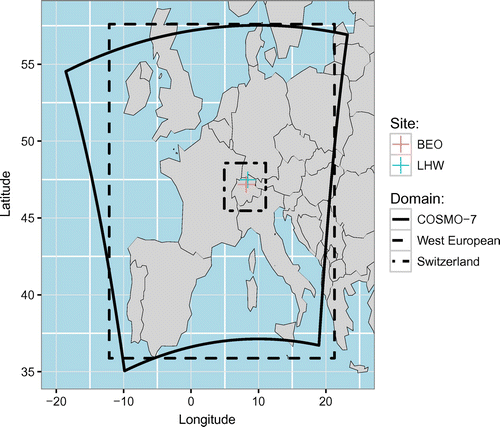
FLEXPART-COSMO was run in backward mode (receptor-oriented, i.e., simulating upwind surface influence of sites) every 3 hours to simulate the movement and provenance of observed air parcels. In each simulation, 50,000 particles were released from the site’s position at site-dependent heights above ground and traced backward in time 4 days or until they left the simulation domain.

After being scaled with the dry air density , residence times (s m kg) were recorded for a high-resolution output domain over Switzerland (E to E and N to N) at resolution, and a European output domain (E to E and N to N) at resolution. Residence times were then folded with regional surface flux inventories to arrive at dry air mole fractions (Seibert and Frank, 2004), which are estimates of respective regional signals. FLEXPART particle trajectory end points are defined by their time and position at the end of the simulation or when leaving the simulation domain. These endpoints are used to calculate initial and boundary conditions (Section 3.3.2). Further description of FLEXPART-COSMO can be found in Oney et al. (2015). The particle release heights at the observation sites were chosen based on a meteorological evaluation of COSMO in Oney et al. (2015) and are listed in Table 2.

Table 2. Simulation characteristics for two observation sites of the CarboCount CH network. Listed from left to right are observation heights (m above ground level), FLEXPART-COSMO particle release heights (m above model ground level), the ‘true’ site altitudes (m above sea level), smoothed COSMO numerical weather prediction model’s (4 km) site altitude, and the geographic site locations.

Site	Meas. Height	Rel. Heights	Alt.	Alt. COSMO	Lat., Lon.
Beromünster	212	212	797	723	47.1896, 8.1755
Lägern-Hochwacht	32	100–200	840	566	47.4822, 8.3973

3.3.2. Lateral boundary conditions for CO₂

The lateral boundary conditions for atmospheric CO₂ for the European domain were deduced from a global CO₂ atmospheric transport model by interpolating the 3-D CO₂ mole fractions from the temporally closest field to the 50,000 particle trajectory end points of each FLEXPART simulation and computing the average of the interpolated values. Global CO₂ fields were provided by the data assimilation system of the Monitoring Atmospheric Composition and Climate (MACC) project of the European Centre for Medium Range Weather Forecast (ECMWF) (Chevallier et al., 2010; Chevallier, 2013). We used the simulation version MACC-II/v13r1 (Chevallier, 2015) in which global surface observations including those at Jungfraujoch were assimilated, but those of the CarboCount CH sites were not assimilated.

3.3.3. Anthropogenic CO₂ and CO signals

The anthropogenic emission inventories of CO₂ and CO were generated by merging relatively coarse global and European inventories with high-resolution inventories available for Switzerland. For CO₂, the global EDGAR v4.2 FT2010 ‘Fast Track’ inventory (Olivier et al., 2011) available at resolution was merged with a new high-resolution (500 m 500 m) inventory for Switzerland developed by Meteotest LLC (Berne, Switzerland), on behalf of the project CarboCount CH, hereafter referred to as ‘CarboCount’ inventory. The latest year available in both inventories was 2010, but the Swiss inventory was scaled to match the total for 2012 as officially reported to the United Nations Framework Convention on Climate Change (FOEN, 2014). Both emission inventories include the emissions from the burning of fossil fuels, the burning of biomass (wood), and the production of cement.

For CO, the European TNO-MACC II emission inventory (Kuenen et al., 2014) available at approximately 7 km 7 km resolution for the year 2009 was merged with a high-resolution (200 m 200 m) CO inventory of Switzerland from 2005. Due to the large, mostly negative trends in European CO emissions, both inventories were scaled by nation to match officially reported values of the year 2012 (latest year available), while preserving the emission’s spatial distribution. Country totals reported to the Convention on Long-range Transboundary Air Pollution (LRTAP) were obtained from the EMEP/CEIP web database (http://www.ceip.at/). As is the case for CO₂, the emission inventory for CO includes the burning of both fossil and modern fuels, while cement manufacturing does not lead to an emission of CO.

For both CO₂ and CO emissions, temporal profiles describing diurnal, day-of-week and monthly variations were prescribed based on sector-specific profiles developed in the project EURODELTA-II (Thunis et al., 2008), similar to Peylin et al. (2011). These profiles have been developed for a source classification according to SNAP (Standardized Nomenclature for Air Pollutants) codes. However, both EDGAR and the two Swiss inventories are based on different nomenclatures, e.g., the IPCC nomenclature in case of EDGAR. Specific conversion tables were therefore developed mapping the different emission categories onto the most closely matching SNAP codes (Kuenen et al., 2014). In addition, a country mask was applied to the EDGAR inventory, a gridded inventory without national borders, in order to apply country-specific day-of-week and monthly profiles. Diurnal profiles were identical in all countries but were adjusted to the local time in each country. Monthly scaling factors were temporally interpolated between the centers (day 15) of each month. Finally, hourly fields of total (sum over all categories) emissions of CO₂ and CO were reprojected to the two simulation domains, and averaged to three-hourly resolution as used by FLEXPART-COSMO. The anthropogenic CO₂ and CO signals were then simulated with FLEXPART-COSMO.

3.3.4. Biospheric CO₂ signal

In order to evaluate the residual regional biospheric signals inferred from the observations, we also computed this signal directly by using the net ecosystem exchange (NEE) fluxes from the Vegetation Photosynthesis and Respiration Model (VPRM) model as a boundary condition (Mahadevan et al., 2008). NEE represents the net exchange of CO₂ between the atmosphere and the terrestrial biosphere and in the model is equal to photosynthesis minus ecosystem respiration, since this model does not include any perturbation fluxes arising from, e.g., fires or insect outbreak. The fluxes computed by VPRM are driven by satellite and meteorology data. Parameters in VPRM controlling these fluxes had been optimized using CarboEurope-IP eddy covariance flux observations at various sites as described in Pillai et al. (2012). After converting to a surface mass flux and reprojecting to the simulation domain, the hourly NEE fields were averaged to three-hourly resolution, and the biospheric influence on each site was then simulated with FLEXPART-COSMO.

4. Results & discussion

The atmospheric CO₂ mole fractions observed at the two sites Beromünster and Lägern-Hochwacht exhibit the expected annual cycle for the northern hemisphere, with a summertime trough and a wintertime crest (Figs. 2 and 3, panel A). During the warmer months at Lägern-Hochwacht, the daily variation of CO₂ is due to a combination of biospheric activity and atmospheric boundary layer (ABL) dynamics (Oney et al., 2015). Beromünster’s observations show these effects as well, but less strongly, due to a combination of high inlet height and relatively high elevation above the Swiss Plateau owing to its location on top of a hill. Wintertime observations at Beromünster and Lägern-Hochwacht show relatively little diurnal variation, but contain samples of polluted air stretching for periods of days to weeks (Oney et al., 2015; Satar et al., 2016). Being 40.5 km apart, the two sites usually sample related air masses, resulting in similar time series. This also suggests that local influences at the two sites are small.

Figure 2. Observed CO₂ mole fractions (A), observation-based (obs1) and FLEXPART-COSMO-modeled (mod1) CO₂ background (B), anthropogenic (C) and biospheric (D) components at Beromünster during 2013. Also shown in (A) is the sum of all simulated components. For an overview of the settings for obs1 and mod1 see Table 1.

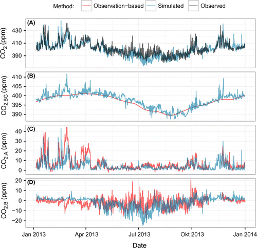
Figure 3. Same as Fig. 2 but at the Lägern-Hochwacht site.

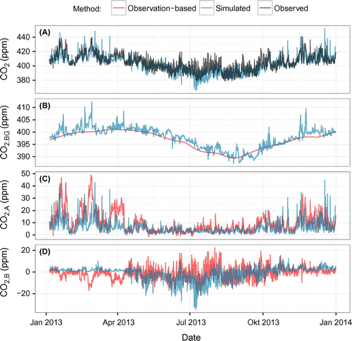
The modeled atmospheric CO₂ mole fractions represent the observations well (Figs. 2 and 3, panel A), but a closer inspection reveals considerable differences in summertime and during a few individual events in winter at both sites. These differences can come from any of the three modeled components, i.e. the background, the anthropogenic, and the biospheric signals. The biospheric signal is presumably the most uncertain component, since uncertainties in background concentrations simulated by global CO₂ data assimilation systems are typically below 1 ppm (Babenhauserheide et al., 2015) and uncertainties in anthropogenic CO₂ emissions are comparatively small, e.g. only 2 % for annual mean emissions from Switzerland (FOEN, 2014).

4.1. Background signals of CO₂ & CO

Background sites such as Jungfraujoch are defined by their lack of local influence owing to them being far away from any anthropogenic emissions. Consequently, the mole fraction of CO is considerably lower at Jungfraujoch relative to Beromünster or Lägern-Hochwacht, where the proximity to CO sources is apparent (Fig. 4). Therefore, background CO signals estimated directly from Beromünster or Lägern-Hochwacht observations are typically greater than when Jungfraujoch is used as a background. Wintertime CO₂ background signals from Beromünster and Lägern-Hochwacht are also greater than those from Jungfraujoch owing to frequent sampling of polluted air with elevated mole fractions of anthropogenic CO₂ at Beromünster and Lägern-Hochwacht and reduced vertical mixing in this season. On the other hand, even though the air sampled at the high Alpine site Jungfraujoch exhibits little influence from Switzerland (Henne et al., 2010), summertime Jungfraujoch CO₂ background signals differ little from the observations at Beromünster or Lägern-Hochwacht. This may partly be due to a balancing of anthropogenic emissions and biospheric uptake, but is mainly due to enhanced vertical mixing.

Figure 4. CO₂ (panels A–B) & CO (panels C–D) measured mole fractions (black and gray) and ‘robust estimate of baseline signal’ (REBS) estimates (red and orange) at Beromünster, Lägern-Hochwacht, and Jungfraujoch (JFJ) during 2013. The REBS background estimates are calculated with a 45-day local regression window.

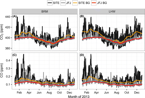
The Jungfraujoch CO₂ background signal overall behaves similarly to the modeled background mole fraction at Beromünster or Lägern-Hochwacht, although the Jungfraujoch-based background varies much less than the modeled background (Figs. 2 and 3, panel B). However, as indicated in Section 2, the two background signals are not strictly compatible, because they are defined differently, i.e. with regard to different spatial and temporal domains. In the case of the model-based estimate, the size and structure of the signal depends directly on the size of the model domain (Central Europe) and the backward simulation time period (four days). The large amount of variation in the model-based background (variance ranging from 2–5 ppm during winter and spring to 10–16 ppm during summer and fall; for a discussion of the different components of total observed variance see section 4.4.1) suggests that the domain was too small or the simulation period too short for signatures from remote fluxes to fully dilute into the large-scale background. The correlation of the background signal CO_{2,  BG} with several peaks in the anthropogenic signal CO_{2,  A} suggests that during stagnant weather conditions with strong air pollutant accumulation the air parcels remained in the European ABL longer than only four days.

In contrast, the observation-based background signal from Jungfraujoch attempts to remove all recent influence even if it originated outside the model domain. The fact that this background is much smoother (variance ranging from 0.7–0.9 ppm during winter and spring to 5–7 ppm during summer and fall) suggests that it is representative for a large-scale, well-mixed background that is little affected by fluxes over Europe.

4.2. Anthropogenic CO₂ to CO ratio

The estimation of the apparent anthropogenic CO_{2,  A} to CO_A mole fraction ratio, , is one of the main challenges in the application of the CO-based method. Our standard approach was to use the slope of the wintertime relationship between the regional CO₂ and CO_A signals estimated by using Jungfraujoch as a background site. Figs. 5B,E reveals that these two signals are indeed highly correlated. To be consistent with previous studies, which reported the apparent ratios of CO to CO₂, we report the ratios here as their inverse . In wintertime, a ratio of 7.750.17 ppb CO/ppm CO₂  for Beromünster and 7.000.27 for Lägern-Hochwacht was observed (see Table 3).

Figure 5. Modeled and measured CO₂ and CO regional signals at Beromünster and Lägern-Hochwacht, colored according to season. Panel A: modeled CO_2,A and CO_A at Beromünster. The slope of the regression line corresponds to of method mod1. Panel B: CO_{2,  R} and CO_A regional signals above a background signal from Jungfraujoch. The slope of the regression line is calculated using only wintertime regional signals and corresponds to of method obs1. Panel C: the same is shown as in panel B except using background estimates from the target site Beromünster (method obs5). Panels D-F: the same as panels A–C shown with regional signals from Lägern-Hochwacht.

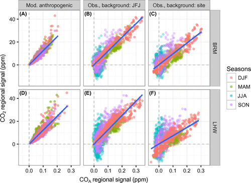
Table 3. Sensitivity of the inverse ratios ( ppb CO/ppm CO₂) to the choice of background signal, and to the choice of local regression window width. The uncertainty of is reported as the confidence interval of the slope from the total weighted least squares regression, forced through the origin. is the coefficient of determination estimated by Pearson’s correlation. The obsN cases included observations from the large-scale pollution event at the end of February, whereas the obsN cases used only the observations during this and a similar event in March/April (see Fig. 6 and Section 4.3).

Site	Case	Window width
		(days)	(ppb/ppm)	(ppb/ppm)
BRM	obs1	30	7.73	0.17	0.97
	obs1	45	7.75	0.17	0.97
	obs1	60	7.75	0.17	0.97
	obs1	45	8.39	0.27	0.96
	obs1	45	9.54	0.43	0.92
	obs5	30	8.95	0.40	0.88
	obs5	45	8.55	0.41	0.87
	obs5	60	8.49	0.41	0.87
	obs5	45	10.00	0.61	0.86
	obs5	45	13.29	1.48	0.65
	obs2,obs6		9.53	0.29	0.80
LHW	obs1	30	6.97	0.27	0.92
	obs1	45	7.00	0.27	0.92
	obs1	60	7.02	0.27	0.92
	obs1	45	7.70	0.39	0.89
	obs1	45	9.70	0.49	0.90
	obs5	30	8.50	0.70	0.69
	obs5	45	8.34	0.73	0.67
	obs5	60	8.45	0.78	0.65
	obs5	45	10.19	1.07	0.64
	obs5	45	14.57	2.24	0.45
	obs2,obs6		8.98	0.33	0.80

Note that two large pollution episodes in late winter (February 19 to 28) and spring (March 20 to April 12) were excluded in the computation of these ratios. As discussed in Subsection 4.3, these pollution events were rather exceptional. Excluding the events results in ratios more consistent with those reported by Satar et al. (2016) (Table 4), which are based on the same observations at Beromünster but are representative for a longer analysis period including the year 2014. Including these events would result in about 20 % higher ratios ( and in Table 3), suggesting a significant sensitivity to the choice of analysis period.

For Beromünster, Satar et al. (2016) showed that in contrast to the high CO : CO₂ correlation in wintertime the correlations are substantially weaker during the other seasons. Springtime ratios are marked by decreasing regional CO₂ likely related to initial plant growth, and high CO_A signals are likely related to domestic heating (Fig. 5B,E). In summer, the correlation weakens further due to the large and highly variable contribution of the net biospheric signal combined with weak CO_A signals. Observed autumn ratios reflect the weakening biopheric signals owing to smaller production and possibly increased litter decomposition combined with increasingly strong CO_A; i.e. they portray the gradual change from summer to winter. During winter, the correlation is strong suggesting that the biospheric influence is small and that regional CO₂ is driven mainly by human-induced combustion.

As expected, the correlations between the simulated CO_{2,  A} and CO_A remain strong throughout the year, as these simulated signals are purely driven by the anthropogenic emissions of CO₂ and CO (Fig. 5A,D). The variability in the modeled relationship reflects variations in air mass origin and the corresponding influence of the spatially variable CO₂ to CO emission ratios across Europe, as well as differences in the temporal variations of CO₂ and CO emissions. Nonetheless, these varying processes do not lead to substantial seasonal variations in the slope between the modeled CO_{2,  A} and CO_A. This supports the idea that observed wintertime estimates may be representative for the entire year (Table 3). However, the studies of van der Laan et al. (2010) and Vogel et al. (2010) based on the radiocarbon-CO method reported a non-negligible seasonal variation of the ratios of CO to fossil fuel CO₂.Based on seven years of observations in the city of Heidelberg, for example, Vogel et al. (2010) found approximately 10% lower ratios in winter than in summer.

Beromünster is located in a rural area where wood is frequently used for domestic heating and farm vehicle emission regulations are less strict than those for road traffic. Lägern-Hochwacht, on the other hand, is located in a relatively more densely populated and industrialized area, where combustion tends to be more efficient. The simulated apparent ratios reflect the expectation that air parcels observed at Beromünster ( of 9.53 0.29) are more CO-enriched than those at Lägern-Hochwacht (8.98 0.33). Correspondingly, the observed air parcels at Beromünster tend to be more CO-enriched than those at Lägern-Hochwacht. These ratios are slightly higher than the annual mean emission ratio of 8.3 of the underlying CO and CO₂ inventories for the domain of Switzerland. Modeled ratios derived from weekly instead of annual relationships range from 7.55 to 12.60 (median of 9.35)  ppb CO/ppm CO₂  at Beromünster, and from 6.93 to 11.20 (median of 8.79)  ppb CO/ppm CO₂  at Lägern-Hochwacht, respectively (see Subsection 4.3).

The observation-based ratios are relatively insensitive to the choice of the smoothing window required to determine the background signals in CO and CO₂, but react sensitively to the choice of the background site (Table 3). If the site’s observations are used to determine the background signals, then the ratios increase, largely owing to the regional signal in CO₂ during wintertime being smaller relative to that for CO (Fig. 4). In other words, this is caused by the site baseline for CO₂ being considerably larger than the JFJ baseline for CO₂, whereas the CO baseline estimates remain closer together.

Taking the baseline from Jungfraujoch implicitly assumes that the air masses at the sites BRM and LHW have the same origin as those at Jungfraujoch. However, even if this is not always the case, using the same background observation site for both CO₂ and CO has the potential to compensate for issues arising from different air mass origins. If, for example, the true CO background at Beromünster during a given period was larger than the one at Jungfraujoch, the same would likely hold for CO₂, and if the CO:CO₂ ratio between these differences in background was the same as the ratio of the regional enhancements, this would be compensated in the computation of the biospheric CO₂ component using Equation (4).

When comparing our results of with previously reported fossil fuel based CO_A/CO_{2,  FF} ratios (Table 4), our results are mostly smaller with the exception of two sites in coastal and remote environments. However, it needs to be emphasized that these results are not always directly comparable, as they refer to different periods, regions, and methodologies. Our anthropogenic components (CO_{2, A} and CO_A) include also the contribution of the combustion of non-fossil, carbonaceous materials, resulting in lower ratios as compared to -based methods which do not include these emissions. Due to wood-burning, the use of biofuels, and waste incineration (Mohn et al., 2008), non-fossil combustion in Switzerland constitutes 14 % of CO₂ emissions according to the Swiss national emission inventory (FOEN, 2014). Additionally, owing to many technological advances since the time of the outlined studies, the combustion efficiency has increased resulting in proportionally less CO being emitted, which further reduces the ratio.

Table 4. Summary of observed ’s found in previous studies. The upper portion of the table displays long-term observation results, and the lower half of the table displays observation campaign results. CO_A/CO_2,R refers to ratios calculated from continuous CO₂ and CO observations above background, analogous to this study. CO_A/CO_{2, FF} indicates fossil fuel CO₂ (CO_{2, FF}) calculated from (see Levin et al. 2003). The information used for the method is presented as the apparent ratio calculation, background, and the metric shown. The units of are  ppb CO/ppm CO₂.

	Location	Period	Method	Study
12.40.5	Harvard forest, USA	1996 Wintertime	COA/CO2,A, monthly percentile, mean and standard deviation of three months	Potosnak et al. (1999)
12.20.4	Heidelberg urban site, Germany	2001-09–2004-04	COA/CO2,FF, Jungfraujoch & GLOBALVIEW-CO, mean and standard deviation	Gamnitzer et al. (2006)
15.55.6  & 14.65.5	Heidelberg urban site, Germany	2002–2009	COA/CO2,FF, Jungfraujoch, weighted mean and standard deviation & median and interquartile range	Vogel et al. (2010)
95	Lutjewad coastal site, Netherlands	2006–2009	COA/CO2,FF, Jungfraujoch, mean standard deviation	van der Laan et al. (2010)
11.29  & 12.211  & 11.98	Coastal northeast USA	2004–2010; annual, summer, and winter	COA/CO2,FF; Free troposphere observations, median and uncertainty (average of uncertainty range)	Miller et al. (2012)
	Beromünster tall tower, Switzerland	2012–2014	COA/CO2,R (above seasonal harmonics estimates), standard major axis regression	Satar et al. (2016)
6.82.2  & 11.75.5	Niwot Ridge mountain site, USA	2004-01-20 & 2004-03-02	COA/CO2,FF, average from 2003-11–2004-04 with western winds, mean and standard deviation	Turnbull et al. (2006)
11.22  & 142	Sacramento metropolitan area, USA	2009-02-27 & 2009-03-06	COA/CO2,FF, Free troposphere observations, linear regression slope	Turnbull et al. (2011)
56 (33)  & 22 (20)	Downwind of China and Japan, respectively (outliers removed)	2001-02-24 to 2001-04-10	COA/CO2,A, none, reduced axis regression	Suntharalingam et al. (2004)

4.3. Anthropogenic CO₂

The anthropogenic component CO_{2,  A} is a considerable component of total CO₂ at the two observing sites of the CarboCount CH network (Figs. 2 and 3, panels B). In the ‘obs1’ base case during winter, CO_{2,  A} variability dominates the atmospheric CO₂, constituting 94–124 % (85–91 ppm) of the total observed variance in wintertime (see Section 4.4.1; values larger 100 % can occur due to negative covariance of the contributing signal components). In summertime, the signals are substantially weaker at around 9 % (3–5 ppm) of total summertime variance, not because of weaker emissions but largely because of increased vertical mixing in the lower troposphere.

The observation-based estimate of the anthropogenic CO₂ component looks plausible when compared to the simulated anthropogenic signal (mod1) for the whole year of 2013 (Figs. 2 and 3, panel C). In fact, the directly modeled anthropogenic signals (mod1) agree remarkably well with the estimates derived from the CO observations (obs1). The largest differences occur during wintertime and early spring, arising from any combination of errors in transport and mixing, and in the emission inventories of CO and CO₂ (Fig. 6).

Figure 6. Spatially disaggregated modeled and observed regional CO : CO₂ ratios for late winter- and springtime pollution events during which neither observation-based nor modeled estimates explain the observed CO₂ at Beromünster and Lägern-Hochwacht. The disaggregation followed the method by Stohl (1996) (see Section 4.3). It was only applied to surface sensitivities above a threshold which denotes an isoline enclosing 90 % of the cumulative sum of surface sensitivities (see Oney et al. 2015) from the respective time periods.

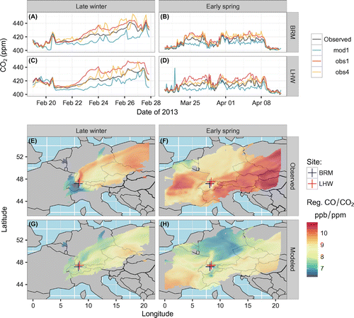
To investigate the potential contribution of errors in the emissions of CO and CO₂ to the largest mismatches, we analyzed the possible dependence of the CO : CO₂ ratios on the air mass origin during two of the large pollution events mentioned earlier, the first one being referrred to as ‘late winter’ (February 19–28, 2013) and the second one as ‘early spring’ (March 20 to April 12, 2013). To this end, a regional CO : CO₂ ratio map during these two anomalous periods was calculated by distributing the observed regional CO₂ and CO signals over the concurrent simulated surface sensitivities applying the trajectory statistics method of Stohl (1996), as in:(8)

where is the measured mole fraction above background at time l and are the scaled residence times computed with FLEXPART-COSMO for each grid cell (i, j) and the summation runs over all observations during a given period. For each time period, this was performed by combining the average mole fraction fields of CO and CO₂ produced by the trajectory statistics method for both sites separately and dividing the resulting and fields by each other. The same was done with the modeled regional anthropogenic signals (Fig. 6, panels E–H).

During these pollution events, cold, northeasterly winds brought highly CO-enriched air from Eastern Europe resulting in anomalously high CO : CO₂ ratios, which differ substantially from the ratios observed during the rest of the winter. As a result, applying the mean wintertime ratio (obs1) results in an overestimation of CO₂ during these events (Figs. 6, panels A–D). Applying the three-hourly simulated ratios (obs4) to convert observed regional CO_Ato CO_{2,  A} results in a similar overestimation of CO₂ since these ratios are on average close to . Comparing the spatial pattern of observation- and model-based ratios (Fig. 6) suggests that the CO to CO2 emission ratios over Eastern Europe are significantly underestimated by the inventories. Note that this finding would not change when replacing the CO inventory from TNO/MACC for 2009 by the EDGAR v4.2 inventory available for 2008, since the latter is only 7 % higher on average over Eastern Europe.

A general underrepresentation of CO emissions over Europe during winter was recently also reported by Stein et al. (2014) and Giordano et al. (2015). A large share of coal and wood for domestic heating is likely responsible for large CO : CO₂ emission ratios in the eastern portions of Europe, specifically during the cold seasons.

In contrast to the CO₂ signals estimated from the CO-observations, the directly simulated CO₂ mole fractions (mod1) during these events are lower than those observed (Fig. 6, panels A–D). This suggests that either the emissions were generally underestimated or that the air pollutant accumulation in the ABL was not properly represented by the simulations during these events.

4.4. Biospheric signal

4.4.1. Evaluation

In this section, we evaluate the observation-based (especially obs1) and model-based (mob1) residual biospheric signals by comparing statistical distributions and variances with the directly simulated values (mod1) as a measure of plausibility. We focus on afternoon (1200–1500 UTC) values when the daytime ABL is fully established, since these conditions can be better represented by atmospheric transport models than the stable nocturnal boundary layer (e.g. Goeckede et al., 2010; Tolk et al., 2011; Meesters et al., 2012).

The VPRM-based modeled signals (mod1) follow the expected seasonal trend with slightly positive values in winter and pronounced negative values in summer (Fig. 7). During wintertime, the biospheric signal is expected to be small and positive, due to photosynthesis being negligible and both plant and soil respiration being weak. The time-series during winter (Fig. 8) and the distribution of VPRM-based biospheric signals (Fig. 9A,E) fulfill these expectations. During the growing season, the simulated biospheric signal becomes mostly negative due to net photosynthetic uptake of CO₂ (9C,G).

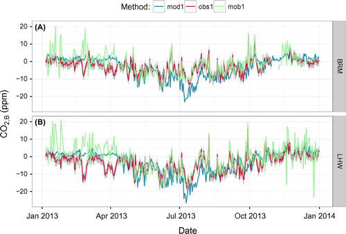
Figure 7. Afternoon (1200–1500 UTC) biospheric CO₂ signals at Beromünster and Lägern-Hochwacht during 2013. The modeled (mod1) and observation-based (obs1) biospheric signals (CO_2,B) are also shown in panel D of Figs. 2 & 3. The model-based residual biospheric signal (mob1) is the residual of measured CO₂ after subtracting the modeled background and anthropogenic signals. The uncertainty (gray) enveloping the residual biospheric signal (obs1) accounts for the uncertainty introduced by the observation based background and anthropogenic CO₂ signals.

In order to assess the contribution of the different components to the overall variability of CO₂ in the different seasons, we computed the variances and covariances of the afternoon (1200–1500 UTC) CO₂ components (Fig. 10). To compare the model- and observation-based approaches, this was done separately for cases obs1 and mob1. Note that in case mob1 the biospheric signal is represented by the residual (observed CO₂ minus simulated background and anthropogenic CO₂) rather than the directly simulated biospheric signal from VPRM. The use of afternoon values removes the variance contribution from diurnal variability. The contributions of the individual components are similar in obs1 and mob1 in summer and autumn but differ strongly in the other seasons.

The observation-based estimate of the biospheric signal (obs1) is consistent with the expected weak release of CO₂ during winter and uptake during the spring to fall period (Fig. 7), reflecting the seasonal cycle of the balance between photosynthesis and ecosystem respiration, i.e., NEE. During summertime, the biospheric signal CO_{2,  B} dominates the variability in atmospheric CO₂, constituting 84–91  (31–55 ppm) of the total summertime variance (Fig. 10). In wintertime, the signals are substantially weaker and constitute only 4–11 % (4–11 ppm) of total variance.

Comparing the wintertime model-based residual biospheric signal (mob1) with the simulated signals shows unrealistically large differences (bias-corrected RMSE [BRMSE] of mob1 vs. mod1; BRM: 28.2 ppm & LHW 50.4 ppm), which results from the inability to correctly represent CO_{2,  BG} and CO_{2,  A} mole fractions. The observation-based biospheric signals (obs1-obs4) are considerably closer to the expected biospheric signal with much less scatter (BRMSE of obs1 vs. mod1; BRM: 4.8 ppm & LHW: 11.2 ppm). Furthermore, the variances of the mob1 biospheric signal are almost as large in winter as in summer (Fig. 10), which again seems implausible.

During the late winter and spring pollution events, when CO-enriched air masses were advected from Eastern Europe (see subsection 4.3 and Fig. 6), both observation- and model-based methods failed to yield realistic residual biospheric signals (February 18–28 in Fig. 8). Better representing the enhanced CO: CO₂ ratios during these events would likely improve both estimates of the residual biospheric signal.

Figure 8. Comparison of biospheric CO₂ signals (CO_2,B) at Beromünster (panel A) and Lägern-Hochwacht (panel B) during the period of 2013-01 – 2013-03.

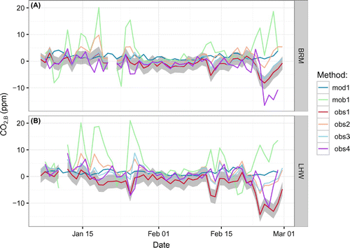
Figure 9. Comparison of the statistical distributions (box and violin [kernel density] plots) of afternoon (1200–1500 UTC) CO₂ biospheric signals at Beromünster (panels A–D) and Lägern-Hochwacht (panels E–H) during 2013, summarized by season for each method (Table 1). JFJ-bg and site-bg denote the distributions of all biospheric signals resulting from the site’s or Jungfraujoch REBS (JFJ-bg includes obs1), respectively. The mean of each distribution is marked by a diamond. The model-based residual biospheric signal (mob1) is the residual of measured CO₂ after subtracting the modeled background and anthropogenic signals.

Figure 10. Afternoon (1200–1500 UTC) CO₂ signal variances at Beromünster and Lägern-Hochwacht during 2013. The model-based CO₂ signal variances (mod1/mob1) are calculated from the respective anthropogenic, biospheric, and background components. The covariance contribution included in the figure gives the sum of the three covariances between the three components. The model-based residual biospheric signal (mob1) is used instead of the modeled biospheric signal (mod1) to be comparable with the observation-based residual biospheric signal (obs1).

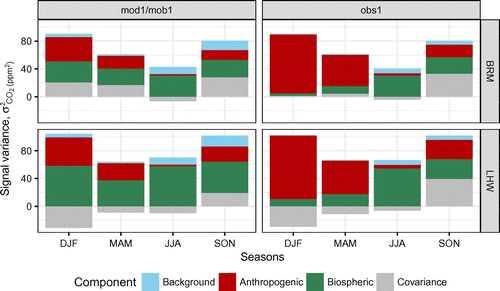
Figure 11. Observed afternoon (1200–1500 UTC) biospheric CO₂ signals (obs1) along with temperature (average of past 24 hours), photosynthetically active radiation (PAR) accumulated over the past 24 hours, as well as precipitation accumulated over the previous 21 days (as a proxy of soil moisture), during the main growing season (01 May–01 September) of 2013 interpolated from COSMO-2 analysis fields to the observation site positions, Beromünster and Lägern-Hochwacht at 250 m above model ground level. Shaded areas demarcate periods during which the average temperature of the preceding 24 hours was C.

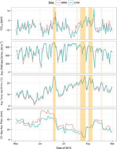
Figure 12. Response of observed afternoon (1200–1500 UTC) biospheric CO₂ signals (obs1) to modeled (described in Fig. 11) PAR, accumulated precipitation, and average temperature at both Beromünster and Lägern-Hochwacht during the growing season (01 May–01 September) of 2013. We narrowed our investigation to convective meteorological situations according to the categorization by Weusthoff (2011). The blue line corresponds to a generalized additive model binned by the 95 % confidence interval.

During summertime, the model- (mob1) and observation-based (obs1) residuals are remarkably similar both in terms of temporal structure (Fig. 7) and statistical distributions (Fig. 9C,G). Similarly, the allocation of variation is very similar (obs1 vs. mob1) at both BRM (30.8 vs. 30.7 ppm or 47 %) and LHW (54.8 vs. 57.7 ppm or 82 % of total). The main reason for this similarity is that the anthropogenic signal is small during summer as it is diluted within the well-mixed, deep ABL. For both residual data sets, the summertime mean and median values are clearly negative but the distributions are rather broad and include significant positive excursions Fig. 9C,G.

Compared to mob1 and obs1, the VPRM-based simulated values during summer are much more negative, especially in July (Fig. 7), and show no positive excursions (Fig. 9C,G). During this season, the total model simulated mole fractions (Fig. 2 and 3, panel A) are frequently well below the observations, suggesting that VPRM overestimates the biospheric sink and is, therefore, no reliable reference for the residual biospheric signals.

The observation-based estimates depend on choices made when determining background and anthropogenic CO₂ signals. The choice of observation site used for the background signal was found to have the largest effect on determining both the CO_A and the accompanying and by extension the resulting residual biospheric signals (compare JFJ-bg to site-bg in Fig. 9). The method employing the target site observations for determination of the background and anthropogenic signals (obs5) fails to capture the background CO signal (see Fig. 4). Using the Jungfraujoch observations for determination of the background appears to produce a more reliable estimate of the regional CO₂ component and hence of the residual biospheric signal.

Accounting for weekly or three-hourly time-dependence of the anthropogenic CO₂:CO ratio (obs3, obs4) surprisingly did not significantly improve the wintertime biospheric signals in terms of the expected positive definiteness and generally small variability (Fig. 8). Furthermore, the statistical characteristics are similar within the grouping of the used background (Fig. 9). Ideally, if the temporal and spatial variability of anthropogenic CO and CO₂ emissions were accurately represented in the model, the obs4 method should work best. Such variability, however, appears to be poorly represented in the emission inventories and/or temporal emission profiles. Currently, a fixed annual (obs1 or obs2) appears to be the most robust approach.

Note that by converting CO into anthropogenic CO₂ as done in this study, we implicitly assume that the part of the wintertime CO₂ signal that is correlated with CO is entirely attributable to anthropogenic emissions. However, we know that also is rather strongly correlated with CO in winter (Satar et al., 2016) despite the fact that more than 80 % of its emissions in Switzerland are caused by agriculture (Henne et al., 2016) and not by combustion sources as in the case of CO. This indicates that the co-variation of tracers is not only the result of correlated emissions but also of the alternation between different weather conditions leading to more or less accumulation of tracers in the ABL irrespective of their origin. Therefore, it is possible that part of the correlated CO₂ signal originates from respiration fluxes rather than anthropogenic emissions. The weakly positive values of the simulated biospheric signal from VRPM in winter (mod1, Fig. 9A,E) indeed suggests nonzero respiration fluxes in this season. As a consequence, the anthropogenic CO₂ signal deduced from CO is likely too high and the residual biospheric signal too small. The fact that the observation-based residuals obs1 are close to zero rather than positive (Fig. 9A,E) is consistent with this assessment. The analysis of the biweekly radiocarbon samples collected at Beromünster will likely shade more light on these questions (Berhanu et al., 2017).

The estimated uncertainty of the observation-based residual biospheric signal (obs1) as indicated by the grey areas in Figs. 7 and 8) consists mostly of the uncertainty of the background (constant estimate from REBS of  ppm) and the uncertainty of the anthropogenic CO₂ signals (on average  ppm). However, the simplifying assumptions of atmosphericCO chemistry and application of a fixed annual likely result in artificially low estimates of the biospheric signal’s uncertainty, which varies little around an average of 2.5 ppm at both sites.

4.4.2. Relation to environmental factors

Next, we address whether the variations in the observation-based biospheric residual (obs1) can be plausibly related to environmental drivers. In general, net photosynthesis has been found to be controlled by available photosynthetically active radiation (PAR), soil moisture, CO₂, nutrients, and leaf level temperature (Bonan, 2008). In contrast, heterotrophic respiration is mainly a function of soil temperature and soil moisture. Relationships between these environmental variables and net ecosystem exchange (NEE) were also established by eddy flux covariance measurements, which indicated that the local meteorological variables PAR, temperature, and soil moisture are the most important factors explaining the observed variability (Baldocchi et al., 2001; Baldocchi, 2008; Beer et al., 2010). Here, we analyze our residual biospheric signal during the growing season (May to August) with meteorological variables as extracted from the COSMO-2 model analysis and interpolated to the location of the two measurement sites. The analyzed variables are temperature (averaged over the preceding 24 hours), PAR (accumulated over the preceding 24 hours), as well as precipitation (accumulated over the preceding 21 days) as a proxy of soil moisture.

During the growing season the biospheric residual was mostly negative indicating biospheric uptake of CO₂ (Fig. 11) but also large variations on synoptic time-scales were observed including periods when the biospheric residuals became positive, indicating a net biospheric source of CO₂. Two periods in mid-June and late July/early August with positive biospheric residuals clearly corresponded to especially warm conditions with daily average temperatures between 20 and C and daytime maximum temperatures around C (Fig. 11). At these high temperatures, photosynthetic activity may largely cease since stomata tend to close to avoid excessive transpiration, which may be further assisted by diminished leaf-level water availability. Furthermore, these periods occurred towards the end of the agricultural growing season when a large fraction of crops (esp. cereals) were already harvested and additional hay harvesting may have further reduced photosynthetic uptake by grasslands. This idea concurs with the fact that both sites are mostly sensitive to crop- and grasslands and only partially to forests during summer (Oney et al., 2015). We also observe a lag (1 day) between increasing temperature and the biospheric response i.e. positive biospheric signals, which supports the notion that these environmental factors drive biospheric signal variation.

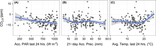
A closer examination of the relationship between the biospheric residuals (obs1) and the environmental variables was carried out by fitting a non-parametric generalized additive regression model (GAM Wood and Augustin, 2002) to the biospheric residuals using the meteorological variables as predictors. This analysis was limited to specific meteorological situations (convective weather and afternoon values 1200–1500 UTC) in order to limit the influence of atmospheric transport and mixing on the observed biospheric residuals. The data from both sites were jointly analyzed in a single GAM, since similar response functions were expected at both sites due to their proximity. We observed the expected relationship between biospheric residuals and PAR with increasingly negative biospheric CO₂ signals with increasing PAR (Fig. 12). For 21-day-accumulated precipitation as a proxy for soil moisture the relationship was less clear but a tendency towards reduced biospheric activity under dry conditions appeared. With temperature, a positive relationship was observed. The combination of the acclimation of plants (Kattge and Knorr, 2007; Groenendijk et al., 2011) to the cold spring, ensuing shock of a short but intense heatwave of June and a sunny rest of the summer (MeteoSwiss, 2014) may help to explain these large and positive biospheric signals during a year with average temperatures (relative to 1981–2010 MeteoSwiss, 2014). Furthermore, these observations may have also been influenced by co-occurrence of these high temperatures with agricultural harvests, particularly of hay.

5. Conclusions

We present a simple and effective method to derive the biospheric signal in atmospheric CO₂ mole fractions using co-located CO₂ and CO observations. Relative to many previous studies, where the biospheric signal was estimated by using model-based estimates of the background and the anthropogenic signals, this method circumvents the introduction of model transport error and inaccuracies of surface flux inventories (as large as 20 % (Peylin et al., 2011)) into the residual. The method combines observations at regionally influenced sites with measurements of the large-scale background at a remote site. The statistical estimate of the background mole fraction at this site does not necessarily have to agree with the boundary conditions of any applied regional-scale transport model, but this difference has to be kept in mind, when using the estimated biospheric signal in inverse modelling. Deviations from the background caused by regional fluxes are divided into their anthropogenic and natural components using concurrent CO observations, for which the regional contributions are assumed to be dominated by anthropogenic emissions. An apparent anthropogenic CO: CO₂ emission ratio can be deduced from wintertime observations when CO and CO₂ are most strongly correlated () and when biospheric fluxes of CO₂ are relatively weak. We found that estimating the anthropogenic CO₂ component using a single annual CO:CO₂ ratio resulted in realistic residual biospheric fluxes during most of the year except for a few pollution episodes in late winter/early spring 2013, when air masses with unusually high CO:CO₂ ratios were transported from Eastern Europe towards Switzerland. In particular, the results were more realistic than the biospheric residuals deduced by subtracting simulated background and anthropogenic CO₂ signals from the observations. We also tested the option of using model-based instead of observation-based CO:CO₂ ratios by simulating the anthropogenic CO and CO₂ mole fractions at the observation sites. Model-based ratios have the advantage of being available throughout the year potentially capturing seasonal variations, but their applicability strongly depends on the quality of the inventories. The model-based annual mean ratios were similar to the observed ones, but the enhanced ratios observed during the pollution events were not captured by the simulations. This suggests that the spatial or temporal variability in CO:CO₂ emission ratios over Europe is not properly represented by state-of-the-art inventories, which currently limits the applicability of model-based ratios.

This study highlights the advantages of co-located CO₂ and CO observations. Given both increasing and increasingly uncertain anthropogenic emissions (Ballantyne et al., 2015), this method might also provide an approach complementing the -based method of investigating CO_{2,  A} (Gamnitzer et al., 2006; Vardag et al., 2015). As also pointed out in our study, the approach has some caveats such as the uncertainty associated with the secondary production of CO from VOC oxidation, which should be investigated in more detail. Improvements to the existing CO emission inventories would also be desirable as mentioned above. Collocated satellite observations of column-integrated CO and CO₂ could help better constrain the emission ratios over different regions.

To further improve the attribution of CO to biospheric and combustion contributions, it would be useful to combine the information gained from the CO measurements with additional tracers such as carbonyl sulfide or stable isotopes of CO. Since CO:CO₂ emission ratios are generally larger for biomass burning than for fossil fuel sources and since the share of biofuels is likely to increase in the future, measurements of a biomass burning marker such as acetonitrile could also be beneficial. Ultimately these measurements will help in better isolating the biospheric signal, and in the end hopefully reduce the uncertainty of the inversely estimated sources and sinks of atmospheric CO₂ over terrestrial systems. Because anthropogenic CO₂ emissions constitute the largest net CO₂ flux of Europe (Ciais et al., 2010a), an emission verification system would bolster mitigation efforts. Co-located CO₂ and CO observations would contribute much to such a verification system.

Acknowledgements

We thank Christoph Gerbig for discussions, provision of the VPRM NEE flux data, and his very helpful comments on an earlier draft of this paper. We thank Frederic Chevallier for providing global CO₂ reanalysis fields (MACC-II, v13r1). The FLEXPART-COSMO simulations were conducted at the Swiss National Supercomputing Center CSCS under project s429. We also acknowledge MeteoSwiss for the provision of their operational COSMO analysis products.

Additional information

Funding

This study was funded by the Swiss National Funds (SNF) as part of the ‘CarboCount CH’ Sinergia Project (Grant Number: CRSII2_136273). We acknowledge the use of the trace gas observations carried out by Martin Steinbacher, Empa, at the High Altitude Research Station Jungfraujoch run by the International Foundation (HFSJG), in the framework of the Integrated Carbon Observation System in Switzerland (ICOS-CH), SNF Grant 20FI21_1489921.

Notes

No potential conflict of interest was reported by the authors.

1 http://www.esrl.noaa.gov/gmd/ccgg/globalview

References

- Acosta Navarro, J. C., Smolander, S., Struthers, H., Zorita, E., Ekman, A. M. L. and co-authors. 2014. Global emissions of terpenoid VOCs from terrestrial vegetation in the last millennium. J. Geophys. Res.: Atmos. 119(11), 6867–6885. DOI:10.1002/2013JD021238.
- Babenhauserheide, A., Basu, S., Houweling, S. and Peters, W. 2015. Comparing the carbontracker and tm5-4dvar data assimilation systems for co surface flux inversions. Atmos. Chem. Phys. 15(17), 9747–9763. DOI:10.5194/acp-15-9747-2015. Online at: http://www.atmos-chem-phys.net/15/9747/2015/
- Baker, D. F., Law, R. M., Gurney, K. R., Rayner, P., Peylin, P. and co-authors. 2006. TransCom 3 inversion intercomparison: Impact of transport model errors on the interannual variability of regional CO2 fluxes, 1988–2003. Global Biogeochem. Cycles. 20(GB1002), 1–17. ISSN 08866236. DOI:10.1029/2004GB002439. Online at: http://doi.wiley.com/10.1029/2004GB002439
- Baldocchi, D. 2008. TURNER REVIEW No. 15’.Breathing’of the terrestrial biosphere: Lessons learned from a global network of carbon dioxide flux measurement systems. Aust. J. Bot. 1–81. Online at: http://www.publish.csiro.au/?paper=BT07151
- Baldocchi, D., Falge, E., Gu, L., Olson, R., Hollinger, D. and co-authors. 2001. FLUXNET: A new tool to study the temporal and spatial variability of ecosystem-scale carbon dioxide, water vapor, and energy flux densities. Bull. Am. Meteorol. Soc. 2415–2434. Online at: http://journals.ametsoc.org/doi/abs/10.1175/1520-0477(2001)0822415:FANTTS2.3.CO;2
- Ballantyne, A. P., Andres, R., Houghton, R., Stocker, B. D., Wanninkhof, R. and co-authors. 2015. Audit of the global carbon budget: Estimate errors and their impact. Biogeosciences 12(8), 2565–2584. ISSN 1726–4189. DOI:10.5194/bg-12-2565-2015. Online at: http://www.biogeosciences.net/12/2565/2015/
- Beer, C., Reichstein, M., Tomelleri, E., Ciais, P. and co-authors 2010. Terrestrial gross carbon dioxide uptake: Global distribution and covariation with climate. Science, 329(5993), 834–838. ISSN 1095–9203. DOI:10.1126/science.1184984. Online at: http://www.ncbi.nlm.nih.gov/pubmed/20603496
- Berhanu, T. A., Satar, E., Schanda, R., Nyfeler, P., Moret, H. and co-authors. 2015. Measurements of greenhouse gases at Beromünster tall tower station in Switzerland. Atmos. Meas. Tech. Discuss. 8(10), 10793–10822. ISSN 1867-8610. DOI:10.5194/amtd-8-10793-2015. Online at: http://www.atmos-meas-tech-discuss.net/8/10793/2015/
- Berhanu, T. A., Szidat, S., Brunner, D., Satar, E., Nyfeler, P. and co-authors. 2017. Estimation of Fossil-fuel Component in Atmospheric CO2 Based on Radiocarbon Measurements at Beromünster Tall Tower. Switzerland: submitted
- Bonan, G. B. 2008. Ecological Climatology: Concepts and Applications, 2nd ed. Cambridge University Press, Cambridge, New York. ISBN 978-0-521-87221-8.
- Broquet, G., Chevallier, F., Rayner, P., Aulagnier, C., Pison, I. and co-authors. 2011. A European summertime CO2 biogenic flux inversion at mesoscale from continuous in situ mixing ratio measurements. J. Geophys. Res.: Atmos., 116(D23303), 1–22. ISSN 01480227. DOI:10.1029/2011JD016202. Online at: http://doi.wiley.com/10.1029/2011JD016202
- Brunner, D., Henne, S., Keller, C. A., Reimann, S., Vollmer, M. K. and co-authors. 2012. An extended Kalman-filter for regional scale inverse emission estimation. Atmos. Chem. Phys. 12(12), 3455–3478. ISSN 1680-7324. DOI:10.5194/acp-12-3455-2012. Online at: http://www.atmos-chem-phys.net/12/3455/2012/%0020, http://atmos-chem-phys-discuss.net/11/29195/2011/acpd-11-29195-2011.pdf
- Chevallier, F. 2013. On the parallelization of atmospheric inversions of CO2 surface fluxes within a variational framework. Geosci. Model Dev. 6(3), 783–790. ISSN 1991-9603. DOI:10.5194/gmd-6-783-2013. Online at: http://www.geosci-model-dev.net/6/783/2013/
- Chevallier, F. 2015. On the statistical optimality of CO2 atmospheric inversions assimilating CO2 column retrievals. Atmos. Chem. Phys. Discus. 15, 11889–11923. DOI:10.5194/acpd-15-11889-2015.
- Chevallier, F., Ciais, P., Conway, T. J., Aalto, T., Anderson, B. E. and co-authors. 2010. CO2 surface fluxes at grid point scale estimated from a global 21 year reanalysis of atmospheric measurements. J. Geophys. Res., 115(D21307), 1–17. ISSN 0148–0227. DOI:10.1029/2010JD013887. Online at: http://doi.wiley.com/10.1029/2010JD013887
- Ciais, P., Paris, J. D., Marland, G., Peylin, P., Piao, S. L. and co-authors. 2010a. The European carbon balance. Part 1: Fossil fuel emissions. Global Change Biology 16(5), 1395–1408. ISSN 13541013. DOI:10.1111/j.1365-2486.2009.02098.x. Online at: http://doi.wiley.com/10.1111/j.1365-2486.2009.02098.x
- Ciais, P., Rayner, P., Chevallier, F., Bousquet, P., Logan, M. and co-authors. 2010b. Atmospheric inversions for estimating CO2 fluxes: Methods and perspectives. Clim. Change 103, 69–92. DOI:10.1007/s10584-010-9909-3. Online at: http://link.springer.com/chapter/10.1007/978-94-007-1670-4\_6
- Crosson, E. R. 2008. A cavity ring-down analyzer for measuring atmospheric levels of methane, carbon dioxide, and water vapor. Appl. Phys. B, 92(3), 403–408. ISSN 0946–2171. DOI:10.1007/s00340-008-3135-y. Online at: http://www.springerlink.com/index/10.1007/s00340-008-3135-y
- Duncan, B. N., Logan, J. A., Bey, I., Megretskaia, I. A., Yantosca, R. M. and co-authors 2007. Global budget of CO, 1988–1997: Source estimates and validation with a global model. J. Geophys. Res.: Atmos. 112(D22301), 1–29. ISSN 01480227. DOI:10.1029/2007JD008459.
- FOEN. 2014. Switzerland’s Greenhouse Gas Inventory 1990–2012. Technical report, Federal Office of the Environment, Bern, Switzerland. Online at: http://www.bafu.admin.ch/klima/13879/13880/14577/15535/index.html?lang=en
- Gamnitzer, U., Karstens, U., Kromer, B., Neubert, R. E. M., Meijer,H. A. J. and co-authors. 2006. Carbon monoxide: A quantitative tracer for fossil fuel CO2? J. Geophys. Res. 111(D22), 1–19. . ISSN 0148-0227. DOI:10.1029/2005JD006966. Online at: http://www.agu.org/pubs/crossref/2006/2005JD006966.shtml
- Gerbig, C., Körner, S. and Lin, J. C. 2008. Vertical mixing in atmospheric tracer transport models: Error characterization and propagation. Atmos. Chem. Phys. 8(3), 591–602. ISSN 1680-7324. DOI:10.5194/acp-8-591-2008. Online at: http://www.atmos-chem-phys.net/8/591/2008/acp-8-591-2008.html
- Gerbig, C., Lin, J. C., Wofsy, S. C., Daube, B. C., Andrews, A. E. and co-authors. 2003. Toward constraining regional-scale fluxes of CO2 with atmospheric observations over a continent: 2. Analysis of COBRA data using a receptor-oriented framework. J. Geophys. Res.: Atmos., 108(D24), 1–14.
- Giordano, L., Brunner, D., Flemming, J., Hogrefe, C., Im, U. and co-authors. 2015. Assessment of the MACC reanalysis and its influence as chemical boundary conditions for regional air quality modeling in AQMEII-2. Atmos. Environ. 371–388. ISSN 13522310. DOI:10.1016/j.atmosenv.2015.02.034. Online at: http://www.sciencedirect.com/science/article/pii/S1352231015001533
- Goeckede, M., Michalak, A. M., Vickers, D., Turner, D. P. and Law, B. E. 2010. Atmospheric inverse modeling to constrain regional-scale CO2 budgets at high spatial and temporal resolution. J. Geophys. Res. 115(D15), 1–23. ISSN 0148-0227. DOI:10.1029/2009JD012257. Online at: http://www.agu.org/pubs/crossref/2010/2009JD012257.shtm
- Goeckede, M., Turner, D. P. and Michalak, A. M. (2010b). Sensitivity of a subregional scale atmospheric inverse CO2 modeling framework to boundary conditions. J. Geophys. Res.: Atmos. 115(24), 1–15. ISSN 01480227. DOI:10.1029/2010JD014443
- Graven, H.D. and Gruber, N. 2011. Continental-scale enrichment of atmospheric 14CO2 from the nuclear power industry: Potential impact on the estimation of fossil fuel-derived CO2. Atmos. Chem. Phys., 11(23), 12339–12349. ISSN 1680-7324. DOI:10.5194/acp-11-12339-2011. Online at: http://www.atmos-chem-phys.net/11/12339/2011/
- Griffin, R. J., Chen, J., Carmody, K. and Vutukuru, S. 2007. Contribution of gas phase oxidation of volatile organic compounds to atmospheric carbon monoxide levels in two areas of the United States. J. Geophys. Res.: Atmos., 112(D10), D10S17. DOI:10.1029/2006JD007602.
- Groenendijk, M., Dolman, a.J., van der Molen, M. and Leuning, R. 2011. Assessing parameter variability in a photosynthesis model within and between plant functional types using global Fluxnet eddy covariance data. Agric. For. Meteorol. 151(1), 22–38. ISSN 01681923. DOI:10.1016/j.agrformet.2010.08.013. Online at: http://linkinghub.elsevier.com/retrieve/pii/S0168192310002273
- Gurney, K. R., Baker, D., Rayner, P. and Denning, S. 2008. Interannual variations in continental-scale net carbon exchange and sensitivity to observing networks estimated from atmospheric CO2 inversions for the period 1980 to 2005. Global Biogeochem. Cycles 22(GB3025),1–17. ISSN 08866236. DOI:10.1029/2007GB003082. Online at: http://doi.wiley.com/10.1029/2007GB003082
- Gurney, K. R., Law, R. M., Denning, A. S., Rayner, P. J., Baker, D. and co-authors. 2003. TransCom 3 CO2 inversion intercomparison: 1. Annual mean control results and sensitivity to transport and prior flux information. Tellus, 55B(2), 555–579. ISSN 0280-6509. DOI:10.1034/j.1600-0889.2003.00049.x. Online at: http://www.tellusb.net/index.php/tellusb/article/view/1672
- Gurney, K. R., Law, R.M., Denning, A.S., Rayner, P. J., Pak, B. C. and co-authors. 2004. Transcom 3 inversion intercomparison: Model mean results for the estimation of seasonal carbon sources and sinks. Global Biogeochem. Cycles, 18(GB1010), 1–18. ISSN 0886623. DOI:10.1029/2003GB002111. http://doi.wiley.com/10.1029/2003GB002111
- Henne, S., Brunner, D., Folini, D., Solberg, S., Klausen, J. and co-authors. 2010. Assessment of parameters describing representativeness of air quality. Atmos. Chem. Phys. 10(8), 3561–3581. ftp://ftp.atmos.washington.edu/pub/ftp/pub/disk/home/sarahd/forbeth/Dec2010Newsletter/GEOmon/Henne\_acp-10-3561-2010.pdf
- Henne, S., Brunner, D., Oney, B., Leuenberger, M., Eugster, W. and co-authors. 2016. Validation of the Swiss methane emission inventory by atmospheric observations and inverse modelling. Atmos. Chem. Phys. 16(6), 3683–3710. DOI:10.5194/acp-16-3683-2016.
- Holloway, T., Levy, H. and Kasibhatla, P. 2000. Global distribution of carbon monoxide. J. Geophys. Res. 105(D10), 12123–12147.
- Hu,, L., Montzka, S. A., Miller, J. B., Andrews, A. E., Lehman, S. J. and co-authors. 2015. U.S. emissions of HFC-134a derived for 2008–2012 from an extensive flask-air sampling network. J. Geophys. Res.: Atmos. 120, 801–825. doi:10.1002/2014JD022617 ISSN 2169-8996
- Hudman, R. C., Murray, L. T., Jacob, D. J., Millet, D. B. and Turquety, S. 2008. Biogenic versus anthropogenic sources of CO in the United States. Geophys. Res. Lett. 35(4), doi:10.1029/2007GL032393http://doi.wiley.com/10.1029/2007GL032393 ISSN 0094–8276
- Kattge, J. and Knorr, W. 2007. Temperature acclimation in a biochemical model of photosynthesis: A reanalysis of data from 36 species. Plant, Cell Environ. 30(9), 1176–1190. ISSN 01407791, 13653040. DOI:10.1111/j.1365-3040.2007.01690.x. Online at: http://doi.wiley.com/10.1111/j.1365-3040.2007.01690.x
- Krystek, M. and Anton, M. 2008. A weighted total least-squares algorithm for fitting a straight line. Meas. Sci. Technol. 19(7), 79801. Online at: http://stacks.iop.org/0957-0233/19/i=7/a=079801
- Kuenen, J. J. P., Visschedijk, A. J. H., Jozwicka, M. and Denier van der Gon, H. A. C. 2014. TNO-MACCII emission inventory; a multi-year (2003–2009) consistent high-resolution European emission inventory for air quality modelling. Atmos. Chem. Phys. 14(20), 10963–10976. ISSN 1680-7324. DOI:10.5194/acp-14-10963-2014. Online at: http://www.atmos-chem-phys.net/14/10963/2014/
- Le Quéré, C., Moriarty, R., Andrew, R. M., Moriarty, R., Peters, G. P. and co-authors. 2015. Global carbon budget 2014. Earth Syst. Sci. Data 7(1), 47–85. DOI:10.5194/essd-7-47-2015http://www.earth-syst-sci-data.net/7/47/2015/ ISSN 1866-3516
- Levin, I. and Karstens, U. 2007. Inferring high-resolution fossil fuel CO2 records at continental sites from combined 14CO2 and CO observations. Tellus B 59B(2), 245–250. ISSN 0280-6509. DOI:10.1111/j.1600-0889.2006.00244.x. Online at: http://www.tellusb.net/index.php/tellusb/article/view/16985%0020, http://onlinelibrary.wiley.com/doi/10.1111/j.1600-0889.2006.00244.x/full
- Levin, I., Kromer, B., Schmidt, M. and Sartorius, H. 2003. A novel approach for independent budgeting of fossil fuel CO2 over Europe by 14CO2 observations. Geophys. Res. Lett. 30(23), 1–5. ISSN 0094-8276. DOI:10.1029/2003GL018477. Online at: http://doi.wiley.com/10.1029/2003GL018477%0020, http://onlinelibrary.wiley.com/doi/10.1029/2003GL018477/full
- Lin, J. C. and Gerbig, C. 2005. Accounting for the effect of transport errors on tracer inversions. Geophysical Research Letters 32(1), 1–5. ISSN 00948276. DOI:10.1029/2004GL021127.
- Mahadevan, P., Wofsy, S., Matross, D. M., Xiao, X., Dunn, A. L. and co-authors. 2008. A satellite-based biosphere parameterization for net ecosystem CO2 exchange: Vegetation Photosynthesis and Respiration Model (VPRM). Global Biogeochemical Cycles 22(GB2005), 1–17.
- Manning, A. J., Ryall, D. B., Derwent, R. G., Simmonds, P. G. and O’Doherty, S. 2003. Estimating European emissions of ozone-depleting and greenhouse gases using observations and a modeling back-attribution technique. J. Geophys. Res. 108(D14), 4405. ISSN 08866236. DOI:10.1029/2006GB002735. Online at: http://doi.wiley.com/10.1029/2006GB002735%0020, http://onlinelibrary.wiley.com/doi/10.1029/2006GB002735/pdf
- Masarie, K. A. and Tans, P. P. 1995. Extension and integration of atmospheric carbon dioxide data into a globally consistent measurement record. J. Geophys. Res. 100(D6), 11593–11610. ISSN 0148-0227. DOI:10.1029/2002JD002312. Online at: http://doi.wiley.com/10.1029/2002JD002312
- Meesters, A. G. C. A., Tolk, L. F., Peters, W., Hutjes, R. W. A., Vellinga, O. S. and co-authors. 2012. Inverse carbon dioxide flux estimates for the Netherlands. J. Geophys. Res.: Atmos. 117(D2030), 1–13. ISSN 0148-0227. DOI:10.1029/95JD00859.
- Mészáros, T., Haszpra, L. and Gelencsér, A. 2005. Tracking changes in carbon monoxide budget over Europe between 1995 and 2000. Atmos. Environ. 39(38), 7297–7306. ISSN 1352-2310. DOI:10.1016/j.atmosenv.2005.09.021.
- MeteoSwiss. 2014. Klimabulletin Jahr 2013. Technical report, Bundesamt für Meteorologie und Klimatologie MeteoSchweiz, Zurich, Switzerland. Online at: http://www.meteoschweiz.admin.ch/home/service-und-publikationen/publikationen.subpage.html/de/data/publications/2014/1/klimabulletin-jahr-2013.html
- Miller, J. B., Lehman, S. J., Montzka, S. a., Sweeney, C., Miller, B. R. and co-authors. 2012. Linking emissions of fossil fuel CO2 and other anthropogenic trace gases using atmospheric 14CO2. J. Geophys. Res.: Atmos. 117(8). ISSN 01480227. DOI:10.1029/2011JD017048.
- Mohn, J., Szidat, S., Fellner, J., Rechberger, H., Quartier, R. and co-authors. 2008. Determination of biogenic and fossil CO2 emitted by waste incineration based on 14CO2 and mass balances. Bioresource Technology 99(14), 6471–6479. ISSN 0960-8524. DOI:10.1016/j.biortech.2007.11.042. Online at: http://www.ncbi.nlm.nih.gov/pubmed/18164616
- Olivier, J., Janssens-Maenhout, G., Peters, J. and Wilson, J. 2011. Long Term Trend in Global CO2 Emissions. Technical report, PBL Netherlands Environmental Assessment Agency and European Commission Publications Office, The Hague (Netherlands).
- Oney, B., Henne, S., Gruber, N., Leuenberger, M., Bamberger, I. and co-authors. 2015. The CarboCount CH sites: Characterization of a dense greenhouse gas observation network. Atmos. Chem. Phys. 15(19), 11147–11164. ISSN 1680-7324. DOI:10.5194/acp-15-11147-2015. Online at: http://www.atmos-chem-phys.net/15/11147/2015/
- Peylin, P., Houweling, S., Krol, M. C., Karstens, U., Rödenbeck, C. co-authors. 2011. Importance of fossil fuel emission uncertainties over Europe for CO2 modeling: Model intercomparison. Atmos. Chem. Phys. 11(13), 6607–6622. ISSN 1680-7324. DOI:10.5194/acp-11-6607-2011. Online at: http://www.atmos-chem-phys.net/11/6607/2011/
- Peylin, P., Law, R. M., Gurney, K. R., Chevallier, F., Jacobson, a. R. and co-authors. 2013. Global atmospheric carbon budget: Results from an ensemble of atmospheric CO2 inversions. Biogeosciences 10(10), 6699–6720. ISSN 1680-7324. DOI:10.5194/acp-11-6607-2011. Online at: http://www.atmos-chem-phys.net/11/6607/2011/
- Peylin, P., Rayner, P.J., Bousquet, P., Carouge, C., Hourdin, F. and co-authors. 2005. Daily CO2 flux estimates over Europe from continuous atmospheric measurements: 1, inverse methodology. Atmos. Chem. Phys. 5(12), 3173–3186. ISSN 1726-4189. DOI:10.5194/bg-10-6699-2013. Online at: http://www.biogeosciences.net/10/6699/2013/
- Pillai, D., Gerbig, C., Ahmadov, R., Rödenbeck, C., Kretschmer, R. and co-authors. 2011. High-resolution simulations of atmospheric CO2 over complex terrain – representing the Ochsenkopf mountain tall tower. Atmos. Chem. Phys. 11(15), 7445–7464. ISSN 1680-7324. DOI:10.5194/acp-11-7445-2011. Online at: http://www.atmos-chem-phys.net/11/7445/2011/
- Pillai, D., Gerbig, C., Kretschmer, R., Beck, V., Karstens, U. and co-authors. 2012. Comparing Lagrangian and Eulerian models for CO2 transport – a step towards Bayesian inverse modeling using WRF/STILT-VPRM. Atmos. Chem. Phys. 12(19), 8979–8991. ISSN 1680-7324. DOI:10.5194/acp-12-8979-2012. Online at: http://www.atmos-chem-phys.net/12/8979/2012/
- Potosnak, M. J., Wofsy, S., Denning, A. S., Munger, J. W. and Barnes, D. H. 1999. Influence of biotic exchange and combustion sources on atmospheric CO2 concentrations in New England from observations at a forest flux tower. J. Geophys. Res. 104, 9561–9569. Online at: http://onlinelibrary.wiley.com/doi/10.1029/1999JD900102/full
- Regnier, P., Friedlingstein, P., Ciais, P., Mackenzie, F. T. and Gruber, N. 2013. Anthropogenic perturbation of the carbon fluxes from land to ocean. Nat. Geosci. 6(8), 597–607. ISSN 1752-0894. DOI:10.1038/ngeo1830. Online at: http://www.nature.com/doifinder/10.1038/ngeo1830
- Rella, C. W., Chen, H., Andrews, A. E., Filges, A., Gerbig, C. and co-authors. 2013. High accuracy measurements of dry mole fractions of carbon dioxide and methane in humid air. Atmos. Meas. Tech. 6(3), 837–860. ISSN 1867-8548. DOI:10.5194/amt-6-837-2013. Online at: http://www.atmos-meas-tech.net/6/837/2013/
- Rigby, M. and Manning, A. J. 2011. Inversion of long-lived trace gas emissions using combined Eulerian and Lagrangian chemical transport models. Atmos. Chem. Phys. 11(18), 9887–9898. . ISSN 1680-7324. DOI:10.5194/acp-11-9887-2011. Online at: http://www.atmos-chem-phys.net/11/9887/2011/
- Roedenbeck, C., Gerbig, C., Trusilova, K. and Heimann, M. 2009. A two-step scheme for high-resolution regional atmospheric trace gas inversions based on independent models. Atmos. Chem. Phys. 9(1), 1727–1756. ISSN 1680-7316. DOI:10.5194/acpd-9-1727-2009
- Ruckstuhl, A. F., Henne, S., Reimann, S., Steinbacher, M., Vollmer, M. K. and co-authors. 2012. Robust extraction of baseline signal of atmospheric trace species using local regression. Atmos. Meas. Tech. 5(11), 2613–2624. . ISSN 1867-8548. DOI:10.5194/amt-5-2613-2012. Online at: http://www.atmos-meas-tech.net/5/2613/2012/
- Sander, S. P., Friedl, R. R., Golden, D. M., Kurylo, M. J., Moortgat,G. K. and co-authors. 2006.. Chemical Kinetics and Photochemical Data for Use in Atmospheric Studies. Technical Report Evaluation Number 15, National Aeronautics and Space Administration, Pasadena, CA,. Online at: http://jpldataeval.jpl.nasa.gov/
- Satar, E., Berhanu, T.A., Brunner, D., Henne, S. and Leuenberger, M. 2016. Continuous CO2/CH4/CO measurements (2012–2014) at Beromünster tall tower station in Switzerland. Biogeosciences 13(9), 2623–2635. ISSN 1726–4189. ISSN 1726-4189. DOI:10.5194/bg-13-2623-2016. Online at: http://www.biogeosciences.net/13/2623/2016/
- Schibig, M. F., Steinbacher, M., Buchmann, B., van der Laan-Luijkx, I. T., van der Laan, S. and co-authors. 2015. Comparison of continuous in situ CO2 observations at Jungfraujoch using two different measurement techniques. Atmos. Meas. Tech. 8(1), 57–68. ISSN 1867-8548. DOI:10.5194/amt-8-57-2015. Online at: http://www.atmos-meas-tech-discuss.net/7/7053/2014/%0020, http://www.atmos-meas-tech.net/8/57/2015/
- Seibert, P. and Frank, A. 2004. Source-receptor matrix calculation with a Lagrangian particle dispersion model in backward mode. Atmos. Chem. Phys. 4(1), 51–63. ISSN 1680-7324. DOI:10.5194/acp-4-51-2004. Online at: http://www.atmos-chem-phys.net/4/51/2004/
- Stein, O., Schultz, M. G., Bouarar, I., Clark, H., Huijnen, V. and co-authors. 2014. On the wintertime low bias of Northern Hemisphere carbon monoxide found in global model simulations. Atmos. Chem. Phys. 14(17), 9295–9316. ISSN 1680-7324. DOI:10.5194/acp-14-9295-2014. Online at: http://www.atmos-chem-phys.net/14/9295/2014/
- Stohl, A. 1996. Trajectory statistics - A new method to establish source-receptor relationships of air pollutants and its application to the transport of particulate sulfate in Europe. Atmos. Environ. 30(4), 579–587. ISSN 13522310. DOI:10.1016/1352-2310(95)00314-2.
- Stohl, A., Forster, C., Frank, A., Seibert, P. and Wotawa, G. 2005. Technical note: The Lagrangian particle dispersion model FLEXPART version 6.2. Atmos. Chem. Phys. 5, 2461–2474.
- Suess, H. 1955. Radiocarbon concentration in modern wood. Science 122(3166), 415–417. DOI:10.1126/science.122.3166.415-a. Online at: http://adsabs.harvard.edu/abs/1955Sci...122..415S
- Suntharalingam, P., Jacob, D. J., Palmer, P. I., Logan, J. A., Yantosca, R. M. and co-authors. 2004. Improved quantification of Chinese carbon fluxes using CO2/CO correlations in Asian outflow. J. Geophys. Res.: Atmos., 109(D18), n/a--n/a. ISSN 2156-2202. DOI:10.1029/2003JD004362. Online at: http://dx.doi.org/10.1029/2003JD004362
- Thoning, K. W., Tans, P. P. and Komhyr, W. D. 1989. Atmospheric carbon dioxide at Mauna Loa Observatory: 2. Analysis of the NOAA GMCC data, 1974–1985. J. Geophys. Res. 94(D6), 8549–8565. ISSN 0148-0227. DOI:10.1029/JD094iD06p08549.
- Thunis, P., Cuvelier, C., Roberts, P., White, L., Post, L. and co-authors. 2008. Evaluation of a Sectoral Approach to Integrated Assessment Modelling including the Mediterranean Sea. Technical report, Joint Research Center, Ispra, Italy. Online at: http://bookshop.europa.eu/de/eurodelta-ii-pbLBNA23444/
- Tolk, L. F., Dolman, A. J., Meesters, A. G. C. A. and Peters, W. 2011. A comparison of different inverse carbon flux estimation approaches for application on a regional domain. Atmos. Chem. Phys. 11(20), 10349–10365. ISSN 1680-7324. DOI:10.5194/acp-11-10349-2011. Online at: http://www.atmos-chem-phys.net/11/10349/2011/
- Turnbull, J. C., Karion, a., Fischer, M. L., Faloona, I., Guilderson, T. and co-authors. 2011. Assessment of fossil fuel carbon dioxide and other anthropogenic trace gas emissions from airborne measurements over Sacramento, California in spring 2009. Atmos. Chem. Phys. 11(2), 705–721. . ISSN 1680-7324. DOI:10.5194/acp-11-705-2011. Online at: http://www.atmos-chem-phys.net/11/705/2011/
- Turnbull, J. C., Miller, J. B., Lehman, S. J., Tans, P. P., Sparks, R. J. and co-authors. 2006. Comparison of 14CO2, CO, and SF6 as tracers for recently added fossil fuel CO2 in the atmosphere and implications for biological CO2 exchange. Geophys. Res. Lett. 33(1), 2–6. ISSN 0094-8276. DOI:10.1029/2005GL024213. Online at: http://www.agu.org/pubs/crossref/2006/2005GL024213.shtml
- van der Laan, S., Karstens, U., Neubert, R., van der Laan-Luijkx, I. T. and Meijer, H. 2010. Observation-based estimates of fossil fuel-derived CO2 emissions in the Netherlands using D14C, CO and 222Radon. Tellus B 62(5), 389–402. ISSN 02806509. DOI:10.1111/j.1600-0889.2010.00493.x. Online at: http://www.tellusb.net/index.php/tellusb/article/view/16582
- Vardag, S. N., Gerbig, C., Janssens-Maenhout, G. and Levin, I. 2015. Estimation of continuous anthropogenic CO2: Model-based evaluation of CO2, CO, d13C(CO2) and D14C(CO2) tracer methods. Atmos. Chem. Phys. 15(22), 12705–12729. ISSN 1680-7324. DOI:10.5194/acp-15-12705-2015. Online at: http://www.atmos-chem-phys.net/15/12705/2015/
- Vogel, F., Tiruchittampalam, B., Theloke, J., Kretschmer, R., Gerbig, C. and co-authors. 2013. Can we evaluate a fine-grained emission model using high-resolution atmospheric transport modelling and regional fossil fuel CO2 observations? Tellus B 1, 1–16. Online at: http://www.tellusb.net/index.php/tellusb/article/view/18681
- Vogel, F. R., Hammer, S., Steinhof, A., Kromer, B. and Levin, I. 2010. Implication of weekly and diurnal 14C calibration on hourly estimates of CO-based fossil fuel CO2 at a moderately polluted site in southwestern Germany. Tellus B 62(5), 512–520. . ISSN 02806509. DOI:10.1111/j.1600-0889.2010.00477.x. Online at: http://www.tellusb.net/index.php/tellusb/article/view/16600
- Weusthoff, T. 2011. Weather Type Classification at MeteoSwiss - Introduction of New Automatic Classification Schemes. Technical Report 235, MeteoSchweiz, Zurich, Switzerlandhttp://www.meteoschweiz.admin.ch/content/dam/meteoswiss/en/Ungebundene-Seiten/Publikationen/Fachberichte/doc/ab235.pdf
- Wood, S. N. and Augustin, N. H. 2002. GAMs with integrated model selection using penalized regression splines and applications to environmental modelling. Ecological Modelling 157(2–3), 157–177. ISSN 03043800. DOI:10.1016/S0304-3800(02)00193-X. Online at: http://linkinghub.elsevier.com/retrieve/pii/S030438000200193X
- Zellweger, C., Forrer, J., Hofer, P., Nyeki, S., Schwarzenbach, B. and co-authors. 2003. Partitioning of reactive nitrogen (NOy) and dependence on meteorological conditions in the lower free troposphere. Atmos. Chem. Phys. 3, 779–796. Online at: http://hal.archives-ouvertes.fr/hal-00295279
- Zellweger, C., Steinbacher, M. and Buchmann, B. 2012. Evaluation of new laser spectrometer techniques for in-situ carbon monoxide measurements. Atmos. Meas. Tech. 5(10), 2555–2567.. ISSN 1867-8548. DOI:10.5194/amt-5-2555-2012. Online at: http://www.atmos-meas-tech.net/5/2555/2012/
- Zhao, C. L. and Tans, P. P. 2006. Estimating uncertainty of the WMO mole fraction scale for carbon dioxide in air. J. Geophys. Res. 111(D08S09), 1–10. . ISSN 0148-0227. DOI:10.1029/2005JD006003. http://doi.wiley.com/10.1029/2005JD006003
- Zondervan, A. and Meijer, H. A. J. 1996. Isotopic characterisation of CO2 sources during regional pollution events using isotopic and radiocarbon analysis. Tellus B 48(4), 601–612. ISSN 0280-6509, 1600-0889. DOI:10.1034/j.1600-0889.1996.00013.x. http://www.tellusb.net/index.php/tellusb/article/view/15934