The particle dry deposition component of total deposition from air quality models: right, wrong or uncertain?

Abstract

Dry deposition is an important loss process for atmospheric particles and can be a significant part of total deposition estimates calculated for critical loads analyses. However, algorithms used in large-scale air quality and atmospheric chemistry models to predict particle deposition velocity as a function of particle size are highly uncertain. Many of these algorithms, although derived from a common heritage, predict vastly different particle deposition velocities for a given particle diameter even under identical environmental conditions for major land use classes. Even more problematic, for vegetated landscapes (forests, in particular) the algorithms do not agree very well with available measurements. In this work, we perform a sensitivity study to estimate how significant the uncertainties in particle deposition algorithms may be in an air quality model’s predictions of ground-level fine particle concentrations, particle deposition and overall total deposition of nitrogen and sulfur. Our results suggest that fine particle concentration predictions at the surface may vary by 5–15% depending on the choice of particle deposition velocity algorithm, while particle dry deposition is affected to a much greater extent with differences among algorithms >200%. Moreover, if accumulation mode particle dry deposition measurements over forests are correct, then dry particle deposition and total elemental deposition to these landscapes may be much larger than is typically simulated by current air quality and atmospheric chemistry models, calling into question commonly available estimates of total deposition and their use in critical loads analyses. Since accurate predictions of atmospheric particle concentrations and deposition are critically important for future air quality, weather and climate models and management of pollutant deposition to sensitive ecosystems, an investment in new dry deposition measurements in conjunction with integrated modelling efforts seems not only justified but vitally necessary to advance and improve the treatment of particle dry deposition processes in atmospheric models.

Keywords:

• dry deposition
• aerosols
• particulate matter
• air quality model
• critical loads

1. Introduction

Accurate predictions of spatial and temporal distributions of atmospheric fine particles are important for air quality research and forecasting (Gong et al., 2015; Lee et al., 2017), climate simulations (IPCC, 2014), and weather forecasting (Grell and Baklanov, 2011; Saide et al., 2015; 2016). Dry deposition to the earth’s surface, including deposition to vegetative canopies, litter-covered surfaces, bare soils, aquatic ecosystems and human-built structures, is an important sink for particles in these modelling systems, especially during periods or in locations with limited precipitation. Moreover, dry deposition of particles is often a substantial component of total deposition (Schwede and Lear, 2014), which is important for assessing the impact of chemical deposition on potentially sensitive ecosystems (Driscoll et al., 2001; Galloway et al., 2003; Pardo et al., 2011; Ellis et al., 2013). In particular, total deposition estimates are required for the calculation of critical load exceedances. A ‘critical load’ is defined as the rate of deposition of a specified pollutant below which harmful effects do not occur for a particular component of an ecosystem. An exceedance occurs if the total deposition rate of the pollutant exceeds the critical load for the ecosystem component of interest. Europe has used the concept of critical loads to manage emissions of selected pollutants for many years (Hettelingh et al., 1995). Although critical loads and exceedance calculations are not required under U. S. law as part of the Clean Air Act, the U. S. Environmental Protection Agency (USEPA) and other federal agencies (e.g. National Park Service, U. S. Forest Service, and U. S. Fish and Wildlife Service) use critical load exceedance calculations as part of larger efforts to understand and manage exposure of sensitive ecosystems across the U. S. to harmful pollutant deposition (U. S. Forest Service, 2011).

Even though the wet deposition component of total deposition is relatively easy to measure and interpolate over broad regions, dry deposition of gases and particles is notoriously difficult to measure (Hicks, 1986), leading to the routine use of inferential methods (i.e. derived from a combination of measured and modelled elements) for the estimation of dry deposition rates (Brook et al., 1997). And, because dry deposition is not spatially ergodic (Hicks, 1995), interpolation of inferentially estimated deposition measurements (i.e. the Clean Air Status and Trends Network – Baumgardner et al., 2002) can be problematic. As a result, three-dimensional air quality or atmospheric chemistry models are typically used to estimate the dry deposition component of total deposition (Ellis et al., 2013; Schwede and Lear, 2014; Lee et al., 2017). For example, the USEPA, in collaboration with the National Atmospheric Deposition Program (NADP) Total Deposition (TDEP) Steering Committee, has created and published spatial maps of total deposition estimates based on a combination of measured and modelled deposition (Schwede and Lear, 2014). The dry deposition portion is computed using modelled deposition velocities from the Community Multiscale Air Quality (CMAQ) model combined with measured concentrations from a variety of surface networks. These total deposition estimates are used for critical loads analyses within the USEPA and are made publicly available for general use and evaluation (https://www.epa.gov/castnet). However, as we attempt to demonstrate in this article, there is considerable uncertainty in model-derived estimates of total deposition, in particular because there is large uncertainty in modelled dry deposition of atmospheric particles. As a result, we argue that current estimates of total deposition are highly uncertain, potentially contain significant underestimates of the deposition of some species to some land use types, and should only be used with caution. Moreover, we further argue that the state of scientific understanding of atmospheric particle deposition is significantly lacking and should be the focus of new, focussed field measurement and integrated modelling studies.

In the sections that follow, we first examine differences in several algorithms commonly used in current air quality and atmospheric chemistry models to predict particle deposition and show how well (or not) these predictions compare with available measurements. Then, as a sensitivity test we implement these algorithms into a common air quality modelling system to see how differences in the particle deposition algorithms affect the model’s overall predictions of surface fine particle concentrations and deposition (dry, wet and total). Further, we implement and test an empirically based particle deposition algorithm that better matches deposition velocity measurements made over forests to gauge how significant known model-measurement discrepancies may be to current model-derived estimates of total deposition. Finally, we discuss the potential importance of our results, especially in light of additional uncertainties in modelling dry deposition processes that have been recognised over the years but which have not been adequately accounted for in air quality and atmospheric chemistry models to date.

2. Models of atmospheric particle deposition

In recent rigorous comparisons of numerous state-of-the-science air quality/atmospheric chemistry models (Solazzo et al., 2012; Im et al., 2015), dry deposition of particles and precursor species was identified as one of the causes of differences in particle concentration and deposition predictions between the models. Of course, in those studies it was difficult to pinpoint the reasons for the observed differences among models, since numerous differences in model components and inputs could have contributed to the variation in results. One possible reason for the differences could be the algorithms that are used in the models to predict particle deposition velocity (since particle removal is the product of both surface concentration and deposition velocity). The algorithms describing particle deposition velocity as a function of particle size in almost all current state-of-the-science air quality modelling systems are descended from the seminal theoretical work of Slinn (1982), Slinn and Slinn (1980) and Slinn (1977). For particle deposition to vegetative canopies, Slinn (1982) formulated the deposition velocity as (1) $$V_d=V_s+\frac{1}{R_a+R_s}$$(1) where, $V_S$ is the gravitational settling velocity of the particle; $R_a$ is the aerodynamic resistance above the surface or vegetative canopy; and, $R_s$ is the surface (or canopy) resistance. The gravitational settling velocity is calculated according to Stokes’ Law via (2) $$V_s=\frac{{\rho }_p{D}_p^{2}g{C}_c}{18\eta }$$(2) where, ${\rho }_p$ is the density of the particle; $D_p^{}$ is the diameter of the particle; $g$ is gravitational acceleration; $C_c$ is the Cunningham correction factor for small particles; and, $\eta$ is the dynamic viscosity of air.

The above-canopy aerodynamic resistance, $R_a$, can be determined via a variety of parameterisations (Liu et al., 2007) but typically is calculated as a function of the canopy roughness length and local atmospheric stability. In Slinn (1982), the surface (or canopy) resistance is calculated as a function of the mean wind speed at the top of the vegetative canopy, $u_h$, the friction velocity, $u_{*}$, an overall canopy collection efficiency, $\epsilon$, and a parameter, $\gamma$, which characterises the shape of the mean wind profile within the canopy (3) $$R_s=\frac{u_h}{u_{*}^2}\frac{1}{\sqrt{\epsilon }}\left\{\frac{1+\sqrt{\epsilon }\tanh \gamma \sqrt{\epsilon }}{\sqrt{\epsilon +\tanh \gamma \sqrt{\epsilon }}}\right\}$$(3)

Slinn (1982) further assumed that the overall canopy collection efficiency was an additive function of separate collection efficiencies resulting from the individual physical processes of Brownian diffusion ($E_B$), interception ($E_{IN}$), and impaction ($E_{IM}$), all modulated by a reduction in collection (R) due to ‘rebound’ of particles back into the atmosphere (4) $$\epsilon =\left(E_B+E_{IN}+E_{IM}\right)R$$(4)

Table 1 presents the functions recommended by Slinn (1982) for calculation of the collection efficiencies and particle rebound. Over the years, other researchers have borrowed the general framework of Slinn (1982), but introduced various modifications and alternative forms for the formulation of $R_s$ and how the individual collection efficiencies are determined.

Table 1. Comparison of Particle Collection Efficiencies for Vegetation Canopies from Selected Algorithms.

Reference	EB	EIN	EIM	R	Other
Slinn (1982)	$\frac{c_v}{c_d}S{c}^{-2/3}$	$\frac{c_v}{c_d}\left[\breve{F}\left\{\frac{D_p}{D_p+\breve{A}}\right\}+\left(1-\breve{F}\right)\left\{\frac{D_p}{D_p+\stackrel{⌢}{A}}\right\}\right]$	$\frac{S{t}^2}{1+S{t}^2}$	$e^{-b\sqrt{St}}$
Zhang et al. (2001)	$S{c}^{-\gamma }$	$\frac{1}{2}{\left(\frac{D_p}{A}\right)}^2$	${\left(\frac{St}{\alpha +St}\right)}^2$	$e^{-\sqrt{St}}$
Pleim and Ran (2011)	$S{c}^{-2/3}$	0	$\frac{{\left({\tau }^{+}\right)}^2}{400+{\left({\tau }^{+}\right)}^2}$	1
Petroff and Zhang (2010)	$c_{B}S{c}^{-2/3}{\mathrm{Re}}_h^{-1/2}$	$\begin{array}{cc}{c}_{IN}\frac{D_p}{L}& \mathit{\text{evergreen}}\\ c_{IN}\frac{D_p}{L}\left[2+\hspace{0.17em}\text{ln}\frac{4L}{D_p}\right]& \mathit{\text{broadleaf}}\end{array}$	$c_{IM}{\left(\frac{St}{{\beta }_{IM}+St}\right)}^2$	1	$\begin{array}{l}{E}_{IT}=\\ \begin{array}{cc}0.0025c_{IT}{\tau }^{+}& {\tau }^{+}<20\\ c_{IT}& {\tau }^{+}\ge 20\end{array}\end{array}$

$A$ = a characteristic length scale for canopy element interception in Zhang et al. (2001) (m).

$\breve{A},\stackrel{⌢}{A}$ = a characteristic width of the “small” and “large” interception collectors, respectively in Slinn (1982) (m).

$b$ = numerical constant in rebound expression – Slinn (1982) recommended = 2.

$c_B$ = LUC-specific coefficient in Brownian collection efficiency expression of Petroff and Zhang (2010).

$c_{IM}$ = LUC-specific coefficient in impaction collection efficiency expression of Petroff and Zhang (2010).

$c_{IN}$ = LUC-specific coefficient in interception collection efficiency expression of Petroff and Zhang (2010).

$c_{IT}$ = LUC-specific coefficient in turbulent impaction collection efficiency expression of Petroff and Zhang (2010).

$\frac{c_v}{c_d}$ = the ratio of the viscous drag coefficient to the total drag coefficient in Slinn (1982).

$D_B$ = the Brownian diffusivity of the particle (m² s⁻¹).

$D_p$ = particle diameter (m).

$E_B$ = particle collection efficiency for Brownian diffusion.

$E_{IN}$ = particle collection efficiency for interception by canopy elements.

$E_{IM}$ = particle collection efficiency for impaction onto canopy elements.

$E_{IT}$ = particle collection efficiency for turbulent impaction.

$\breve{F}$ = the fraction of total interception collection occurring on ‘small’ collectors (i.e. vegetation hairs) in the canopy in Slinn (1982).

$L$ = LUC-specific characteristic length in Petroff and Zhang (2010) (m).

$R$ = reduction in collection caused by particle rebound.

$R{e}_h$ = the Reynolds number at the top of the canopy = $u_{h}L/\nu$.

$Sc$ = the Schmidt number = $v/D_B$.

$St$ = the Stokes number = $V_s{u}_{*}/gl$, where $l$ = $\breve{A}$, $\stackrel{⌢}{A}$, $A$ or $L$, depending on the particular algorithm being used.

$\alpha$ = LUC-specific parameter used in the impaction collection efficiency expression of Zhang et al. (2001).

${\beta }_{IM}$ = LUC-specific parameter used in the impaction collection efficiency expression of Petroff and Zhang (2010).

$\gamma$ = LUC-specific exponent used in the Brownian collection efficiency expression of Zhang et al. (2001).

$v$ = the kinematic viscosity of air (m² s⁻¹).

${\tau }^{+}$ = non-dimensional particle relaxation time used in Pleim and Ran (2011) and Petroff and Zhang (2010); = $StR{e}_{*}$, where $R{e}_{*}$= $u_{*}l/\nu$.

The algorithm described by Zhang et al. (2001) is used in GEM-MACH, Environment and Climate Change Canada’s operational air quality forecast model (Gong et al., 2015), as one of the default options in the Comprehensive Air Quality Model with Extensions (CAMx; Environ International Corporation, 2012), and also in the GEOS-Chem global model (Pye et al., 2009). The Zhang et al. (2001) algorithm, by neglecting within canopy variation of the wind profile (i.e. $\gamma =0$), arrives at a surface resistance of the form (5) $$R_s=\frac{1}{{\alpha }_0{u}_{*}\left(E_B+E_{IN}+E_{IM}\right)R}$$(5) which is equivalent to Equation (3)(3) $$R_s=\frac{u_h}{u_{*}^2}\frac{1}{\sqrt{\epsilon }}\left\{\frac{1+\sqrt{\epsilon }\tanh \gamma \sqrt{\epsilon }}{\sqrt{\epsilon +\tanh \gamma \sqrt{\epsilon }}}\right\}$$(3) and (4)(4) $$\epsilon =\left(E_B+E_{IN}+E_{IM}\right)R$$(4) with $\gamma =0$ and ${\alpha }_0=u_{*}/u_h$. Zhang et al. (2001) specifies a constant value of ${\alpha }_0=3$ for all land use types, although no explanation of this choice is provided. Zhang et al. (2001) also introduced alternative forms for the collection efficiency parameterisations as shown in Table 1, some of which produce efficiencies quite different from the Slinn (1982) choices.

In Pleim and Ran (2011), the authors describe the particle deposition algorithm used in the Community Multiscale Air Quality (CMAQ) model (Byun and Schere, 2006), which also uses the Slinn (1982) framework as a starting point. As in Zhang et al. (2001), Pleim and Ran (2011) neglect the effect of within canopy wind variation and define the surface resistance as (6) $$R_s=\frac{1}{F_f{u}_{*}(E_B+E_{IN}+E_{IM})}$$(6) with, (7) $$F_f=1+0.24\frac{w_{*}^2}{u_{*}^2}$$(7) in which $w_{*}$ is the convective velocity scale. The term $F_f$ is an empirical correction factor, first suggested by Wesely et al. (1985), to account for increased deposition in convective conditions. Pleim and Ran (2011) also employed alternative collection efficiency parameterisations (Table 1), with the notable choice of neglecting the interception collection efficiency (i.e. using $E_{IN}$ = 0), ostensibly because the determination of useful characteristic lengths for vegetation microstructures over a typical model grid cell is troublesome.

Petroff and Zhang (2010) developed an even more complex algorithm based on simplification of a comprehensive one-dimensional aerosol transport model (Petroff et al., 2008a, 2008b, 2009), yet still is loosely derivative from Slinn (1982). In their algorithm, the surface deposition velocity (i.e. $V_s=1/R_s$) is calculated via (8a) $$V_s=E_g{u}_{*}\frac{1+\left[\frac{Q}{Q_g}-\frac{\alpha }{2}\right]\frac{\tanh (\eta )}{\eta }}{1+\left[Q_g+\frac{\alpha }{2}\right]\frac{\tanh (\eta )}{\eta }}$$(8a) with, (8b) $$Q=\frac{LAI{E}_{T}h}{l_{mp}}$$(8b) (8c) $$Q_g=\frac{E_{g}h}{l_{mp}}$$(8c) (8d) $$\eta =\sqrt{{\alpha }^2/4+Q}$$(8d) (8e) $$E_T=\frac{u_h}{u_{*}}\left(E_B+E_{IN}+E_{IM}\right)+E_{IT}$$(8e) where, LAI is the two-sided leaf area index, h is the canopy height, $l_{mp}$ is particle mixing length, $\alpha$ is the aerodynamic extinction coefficient of the canopy, $u_h$ is the mean wind speed at canopy top, $E_g$ is a collection efficiency for deposition to the ground, and $E_{IT}$ is a collection efficiency for turbulent impaction. Table 1 presents the functions used by Petroff and Zhang (2010) to determine $E_B,E_{IN},E_{IM}$ and $E_{IT}$.

Figure 1 illustrates differences in the Slinn (1982), Zhang et al. (2001), Pleim and Ran (2011), and Petroff and Zhang (2010) predictions of particle deposition velocity as a function of particle size and land use category (LUC). All of the models predict a ‘well’ in deposition velocity in the accumulation mode (i.e. the 0.1–2 µm diameter size range) for all land use types, but the particle diameter at which the minimum occurs differs substantially between the models. The minimum in V_d occurs because none of the collection efficiencies are very efficient in this size range, but different expressions for the various efficiencies used by the algorithms result in differences in the diameter at which the minimum occurs (see Fig. S-1 in the Supplement). The Zhang et al. (2001) algorithm predicts a well minimum at a larger diameter (at 2–3 µm) than the other schemes, while the Petroff and Zhang (2010) algorithm predicts a well minimum at the smallest diameter, except for the urban land use type. Pleim and Ran (2011) directly predict little difference in deposition velocity between land use types because the particle interception efficiency, $E_{IN}$, is neglected. However, as seen in Fig. 1, the algorithm is very sensitive to the value of the convective velocity scale, $w_{*}$ (Deardorff 1970), which can vary significantly as a function of the surface roughness, z₀, defined for each land use type. The Petroff and Zhang (2010) algorithm produces the largest differences in predicted deposition velocities among land use types, with urban V_d’s much smaller than produced by the other schemes. For the forest land use types, both Zhang et al. (2001) and Petroff and Zhang (2010) produce higher deposition velocities in the 0.1–2 µm diameter range than Slinn (1982) and Pleim and Ran (2011).

Fig. 1. Comparison of particle dry deposition velocity, V_d (cm s⁻¹), as a function of particle diameter, D_p (µm), for various algorithms and land use types (u* = 60 cm/s for all algorithms and LUCs).

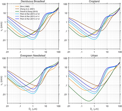
The most striking observation about Fig. 1, however, are the enormous differences in deposition velocities predicted by the various algorithms for a given particle diameter and land use type. For a 0.1 µm diameter particle depositing to a deciduous broadleaf canopy, the Zhang et al. (2001) algorithm predicts a V_d of 0.6 cm s⁻¹, whereas the Petroff and Zhang (2010) algorithm predicts a V_d of 0.023 cm s⁻¹. For a 1 µm diameter particle over a needleleaf evergreen canopy, Petroff and Zhang (2010) predicts V_d = 0.27 cm s⁻¹, while Pleim and Ran (2011) with a w* value of zero predicts V_d = 0.011 cm s⁻¹. Given the common heritage of these algorithms in the formulation of Slinn (1982), the large variation in results between specific formulations is somewhat surprising, but this wide range of behaviour likely helps to explain the results observed by Solazzo et al. (2012) and Im et al. (2015) in their comparisons of current modelling systems.

Several studies have noted over recent years that the algorithms describing the size-dependent dry deposition of atmospheric particles over vegetative canopies do not agree very well with measurements, especially in the accumulation mode, and particularly for canopies with high surface roughness (Zhang and Vet, 2006; Petroff et al., 2008a; Pryor et al., 2008a). Recently, a review by Hicks et al. (2016) surveyed the historical development of both the algorithms and measurements of this phenomenon, noting that measurements as far back as 1977 suggested a pronounced difference between measurements and model-derived expectations. Pryor et al. (2008a) provided a thorough summary of potential explanations for the discrepancies, ranging from observational errors, to chemical flux divergences, faulty model assumptions, or the neglect of important deposition processes (e.g. turbophoresis, thermophoresis, etc.); however, the model-measurement discrepancies remain and have not been definitively settled.

In Figs. 2–6, the algorithms described above are compared to available measurements for five distinct land use types. One immediate observation is that, except for evergreen needleleaf forests, there are only very limited measurements of particle deposition velocity as a function of particle diameter (V_d(D_p)). The large scatter in measurements across all land use types may simply be a reflection of the difficulty of making these kinds of measurements, but also may suggest that other unidentified processes or variables may be affecting particle deposition (e.g. leaf area density distribution as a function of canopy depth, see Katul et al., 2011). Also, the large scatter of data for forest and grassland surface types may possibly account for the wide divergence in model predictions of V_d(D_p), simply depending on which datasets were used in the formulation of a particular algorithm.

Fig. 2. Atmospheric particle deposition velocities (cm s⁻¹) predicted by the four algorithms compared with measurements as a function of particle diameter (µm) for a deciduous broadleaf forest. Error bars represent an estimate of uncertainty either as presented by the respective authors or as derived from the published data. (u* = 40 cm s⁻¹ for all algorithms.).

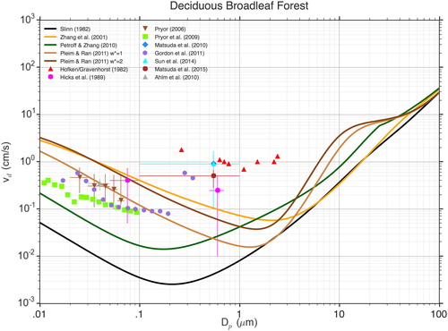
Fig. 3. Atmospheric particle deposition velocities (cm s⁻¹) predicted by the four algorithms compared with measurements as a function of particle diameter (µm) for a evergreen needleleaf forest. Error bars represent an estimate of uncertainty either as presented by the respective authors or as derived from the published data. (u* = 40 cm s⁻¹ for all algorithms.).

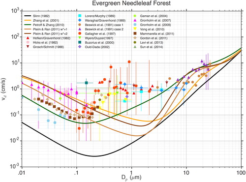
Fig. 4. Atmospheric particle deposition velocities (cm s⁻¹) predicted by the four algorithms compared with measurements as a function of particle diameter (µm) for a grass covered surface. Error bars represent an estimate of uncertainty either as presented by the respective authors or as derived from the published data. (u* = 40 cm s⁻¹ for all algorithms.).

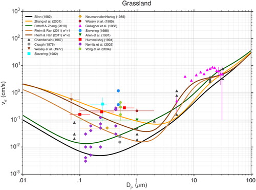
Fig. 5. Atmospheric particle deposition velocities (cm s⁻¹) predicted by the four algorithms compared with measurements as a function of particle diameter (µm) for a water surface. Error bars represent an estimate of uncertainty either as presented by the respective authors or as derived from the published data. (u* = 20 cm s⁻¹ for all algorithms.).

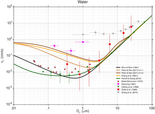
Fig. 6. Atmospheric particle deposition velocities (cm s⁻¹) predicted by the four algorithms compared with measurements as a function of particle diameter (µm) for a snow or ice covered surface. Error bars represent an estimate of uncertainty either as presented by the respective authors or as derived from the published data. (u* = 20 cm s⁻¹ for all algorithms.).

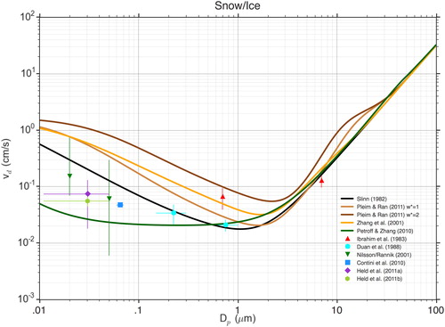
For smooth surfaces, such as water or snow/ice (Figs. 5 and 6), the measurements generally provide some credence to the idea of a minimum in deposition velocity for particles in the accumulation mode, as predicted by most Vd(Dp) algorithms. However, for vegetated surfaces the picture is quite different. For grassland surfaces (Fig. 4), it would be difficult to argue that the measurements provide any evidence for an accumulation mode minimum. The large scatter of measurements in this region also makes it difficult to favour one algorithm over another, although Zhang et al. (2001) and Pleim and Ran (2011) seem to better fit the data over a broader range of particle diameters.

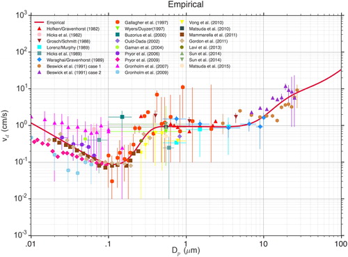
For forested surfaces (Figs. 2 and 3), the data clearly indicate that there is no deposition velocity minimum in the 0.2–2.0 µm particle diameter range. In fact, the data suggest that there may be a minimum somewhere in the 0.1–0.2 µm range, with a sharp rise in V_d between 0.2 and 0.3 µm, rather than the gradual decrease that is predicted by most of the V_d(D_p) algorithms. This is consistent across many of the measurement data sets (Gallagher et al., 1997; Gronholm et al., 2007; Vong et al., 2010; Gordon et al., 2011; Mammarella et al., 2011), but not all (e.g. Buzorius et al., 2000). In any case, none of the models reproduces the measurements in the 0.2–2.0 µm size range for forest surface types, underpredicting V_d by up to two orders of magnitude. This is potentially significant since much of the mass of fine particles is often contained in exactly this size range. As a result, air quality or atmospheric chemistry models that use a V_d(D_p) algorithm similar to the ones shown here will significantly underestimate particle deposition to forested land surface types. Results for grassland surface types suggest that it may be possible that a similar underestimate might occur for all vegetated canopies; however, the sparsity and scatter of the data makes such a statement only speculation.

Given that commonly used algorithms of V_d(D_p) exhibit such wide variation in V_d predictions across land use types and that none of the algorithms do a particularly good job of reproducing available measurements, especially for forest land use types in the accumulation mode, then reasonable questions arise: How important are these uncertainties for air quality model predictions of particle concentration distributions and particle deposition and how might these uncertainties impact total deposition estimates? A series of air quality model simulations, described and presented in the next section, were performed to begin to answer these questions.

3. Particle deposition sensitivity simulations

3.1. Air quality model and domain

Air quality model simulations were constructed to evaluate how the choice of algorithm for particle dry deposition may affect an air quality model’s predictions of PM_2.5 (mass concentration of particles with diameters less than 2.5 micrometers) concentrations and deposition. For these simulations, version 6.0 of the Comprehensive Air Quality Model with Extensions (CAMx; Environ International Corporation, 2012) was selected. CAMx was chosen for this study because its structure allows for easy modification of the particle dry deposition algorithm and because it has the option to simulate aerosols (and hence particle deposition) using a sectional approach. CAMx was configured to use the ACM2 (Pleim, 2007) diffusion scheme, the PPM advection solver and the EBI chemistry solver using the Carbon Bond Mechanism version 5 (Sarwar et al., 2008). The Carnegie Mellon University (CMU) sectional aerosol module was employed with eight size bins (with boundaries of 0.025, 0.054, 0.12, 0.25, 0.54, 1.2, 2.5, 5.4, 11.6 µm) to simulate aerosol processes. The CMU aerosol module as implemented in CAMx uses the Multi-component Aerosol Dynamics Model (MADM; Pilinis et al., 2000) to model condensation, evaporation, coagulation and nucleation processes. Inorganic aerosol thermodynamics are treated using ISORROPIA (Nenes et al., 1998, 1999) and secondary organic aerosol thermodynamics are modelled using the methodology of Koo et al. (2003) and Morris et al. (2005). Deposition velocities were calculated separately for each size bin using the mean bin diameter. Particle dry deposition for each of the algorithms tested was thus a function of particle size and allowed for better comparisons of the differences in the behaviour of the algorithms across the full range of modelled particle diameter.

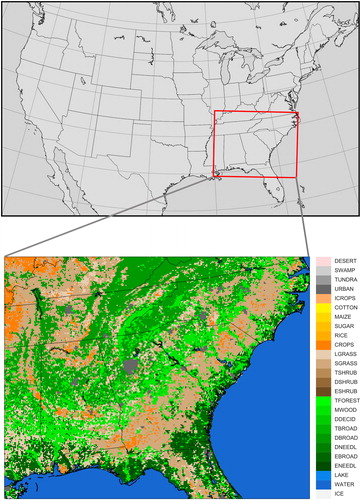
The Southeast U. S. domain shown in Fig. 7 was selected for the study primarily for two reasons: (i) the Southeast is extensively covered by forest (41% of grid cells in the domain are forest land use type, displayed as shades of green in the figure); and, (ii) the existence of a broad range of air quality measurement data sets in the region, including data from the Southern Atmosphere Study (https://www.eol.ucar.edu/field_projects/sas) which took place during the summer of 2013. Simulations were performed over the domain at 4-km horizontal resolution for the 18-day period of June 11–28, 2013, where the first 3 days were used as a spin-up period and results analysed for the 15-day period of June 14–28. Boundary conditions over the period were derived from 12-km CONUS-domain simulations of the NOAA National Weather Service National Air Quality Forecasting Capability (NAQFC; Lee et al., 2017). Meteorological data for both domains were generated using the Non-Hydrostatic Multiscale Model on the B-grid (NMMB), with the 4-km subdomain nested within the 12-km CONUS domain.

Fig. 7. Computational domain consisting of the Southeastern domain (4 km horizontal resolution) nested within the CONUS domain (12 km horizontal resolution) used in the NOAA NWS National Air Quality Forecast Capability.

Emission inputs for the simulations (for both the 12-km CONUS domain and the 4-km Southeast domain) were processed depending on the sensitivity of the sources to meteorology (Tong et al., 2015). For ‘static’ emission sources not strongly influenced by meteorological conditions, including mobile and area sources, the USEPA 2005 National Emission Inventories (NEIs) were used as the baseline emission data set. Mobile emissions and off-road engine emissions for nitrogen oxides (NO_x) were adjusted using the Cross-State Air Pollution Rule (CSAPR) projection factors (Pan et al., 2014), to reflect changes in emissions from the inventory year (2005) to the simulation period (Tong et al., 2015). For point source emission, the NEI05v1 data are used as the base year for Electricity Generation Units (EGUs) and non-EGU point sources. NO_x and sulfur dioxide (SO₂) emissions from EGU sources were upgraded with 2013 Continuous Emission Monitoring (CEM) data. The adjusted inventories were processed using the Sparse Matrix Operator Kernel Emissions (SMOKE) modelling system (Houyoux and Vukovich, 1999) to represent monthly, weekly, diurnal and holiday/non-holiday variations that are specific for each year. For wildfire smoke emissions, fire points and smoke plume locations were identified by the NOAA Hazard Mapping System (HMS) using satellite retrieval and human analysis (Ruminski et al., 2006). The HMS fire smoke products were processed through the U.S. Forest Service BlueSky (version 3.1) framework modelling system (Larkin et al., 2009; O’Neill et al., 2009) to produce near real-time wildfire smoke emissions for the simulations.

3.2. Simulation descriptions

In CAMx, the Zhang et al. (2001) algorithm is one of the selectable options for particle dry deposition. In this work, we implemented the Pleim and Ran (2011) and Petroff and Zhang (2010) algorithms as additional options for particle dry deposition within CAMx. An empirically based algorithm was also implemented in CAMx to explore how total deposition predictions of current air quality models may be affected if deposition velocity measurements over forests are correct. The empirical algorithm was created as a derivative of the Zhang et al. (2001) scheme by forcing the V_d curve as a function of particle diameter for all forest land use types occurring within the domain (evergreen needle, evergreen broadleaf, deciduous broadleaf, and mixed) to more closely represent the measurement data as shown in Fig. 8, in particular matching the data’s lack of a minimum in the accumulation mode above 0.2 µm. This was accomplished by including an additional collection efficiency, $E_{unk}$ for an unknown process into the expression for the surface resistance (9) $$R_s=\frac{1}{{\alpha }_0{u}_{*}\left(E_B+E_{IN}+E_{IM}+E_{unk}\right)}.$$(9)

Fig. 8. Example of the empirical representation of V_d (cm s⁻¹) as a function of particle diameter D_p (µm), using the algorithm of Zhang et al. (2001) but including an additional efficiency for an ‘unknown’ process, thereby forcing the V_d(D_p) function to more closely represent data obtained over forests (u* = 60 cm s⁻¹).

The unknown process collection efficiency was constructed as a logistic equation (see Fig. S-1 and the equation in the Supplement) with particle size as the independent variable so that the resulting V_d(D_p) more closely represented the data as shown in Fig. 8. Using this approach, variation of the other collection efficiencies with respect to input variables (e.g. friction velocity, see Fig. S-2 in the Supplement) remains similar to the original Zhang et al. (2001) algorithm. The unknown collection efficiency was only included in the V_d calculation for grid cells with forested land use types, leaving deposition velocities for grid cells of all other land use types calculated as in the original Zhang et al. (2001) algorithm.

Four simulations were performed in this study for the southeast domain of Fig. 7. The base simulation used the CAMx modelling system with the particle dry deposition scheme of Zhang et al. (2001) selected. Each of the three other simulations used alternate particle dry deposition algorithms: (i) Pleim and Ran (2011); (ii) Petroff and Zhang (2010); and, (iii) the empirical algorithm described above. All other model settings and inputs to the simulations were identical, including boundary conditions (from the CONUS 12 km simulation), emissions and meteorology.

3.3. Results

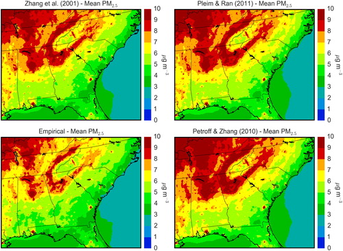
Mean surface concentrations of PM_2.5 over the last 15 days of the simulation (June 14–28, 2013) are shown in Fig. 9 for all four simulations (see also Fig. S-3 in Supplement). There are discernable differences in surface concentrations across the simulations, although in some cases the differences are relatively small. Surface concentration differences between the Pleim and Ran (2011) and base Zhang et al. (2001) simulations range from −2 to +6%, with a domain mean difference of +3.3%. Differences between Petroff and Zhang (2010) and the base run range from +1 to 6%, with a domain mean difference of +5.9%. For the empirical simulation, surface concentration differences between it and the base run range from 0 to −10%, with a domain mean difference of −6.9%. Differences in surface PM_2.5 concentrations between the Petroff and Zhang simulation and the empirical are opposite in sign with respect to the base run and lie in the range of 8–15%. Hourly modelled surface concentrations at individual grid cells over the length of the simulation (see Fig. S-3) have maximum differences from the base run on the order of 5–10%.

Fig. 9. PM_2.5 mean surface concentration (µg m⁻³) for June 14–28, 2013, with PM_2.5dry deposition algorithms of Zhang et al. (2001), Pleim and Ran (2011), Petroff and Zhang (2010), and the empirical algorithm of this work.

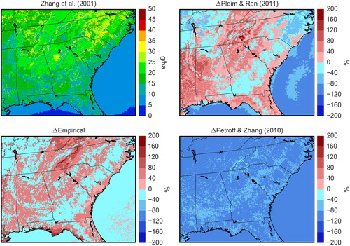
On the other hand, differences with respect to the base simulation in total PM_2.5 cumulative dry deposition over June 14–28 are much more substantial, as seen in Fig. 10 (see also Fig. S-4). The Pleim and Ran (2011) algorithm produced both increases and decreases in PM_2.5dry deposition as compared with the base Zhang et al. (2001) algorithm, ranging from an increase of over 200% to a decrease of nearly 90%, with increases primarily over forested grid cells. Because the Petroff and Zhang (2010) algorithm generally produces smaller particle dry deposition velocities in the accumulation mode, total PM_2.5dry deposition decreases across most of the domain for its simulation as compared to the base run. The empirical algorithm, which attempts to better represent actual deposition velocity measurements over forests, produces PM_2.5dry deposition increases of 120–230% to forest-dominated grid cells. In terms of cumulative PM_2.5dry deposition, Zhang et al. produces a domain mean of 81.6 g ha⁻¹, Pleim and Ran produces a nearly identical 80.6 g ha⁻¹ (−1.2%), Petroff and Zhang produces only 22.5 g ha⁻¹ (−72.4%), and the empirical algorithm produces 142.2 g ha⁻¹ (+74.3%). Averaged over only forested grid cells, the empirical algorithm produces more than 2.4 times the PM_2.5dry deposition (251.6 g ha⁻¹ versus 103.6 g ha⁻¹) than does the Zhang et al. scheme for those cells. Qualitatively similar results are obtained for the dry deposition of PM_2.5 species components sulfate (Fig. 11), nitrate (Fig. 12) and ammonium (Fig. 13).

Fig. 10. Cumulative PM_2.5dry deposition (g ha⁻¹) (June 14–28, 2013) for the base Zhang et al. (2001) simulation and percent differences from the base for each of the tested particle deposition algorithms.

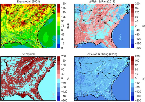
Fig. 11. Cumulative PM_2.5 SO₄²⁻ dry deposition (g ha⁻¹) (June 14–28, 2013) for the base Zhang et al. (2001) simulation and percent differences from the base for each of the tested particle deposition algorithms.

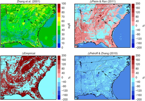
Fig. 12. Cumulative PM_2.5 NO₃⁻ dry deposition (g ha⁻¹) (June 14–28, 2013) for the base Zhang et al. (2001) simulation and percent differences from the base for each of the tested particle deposition algorithms.

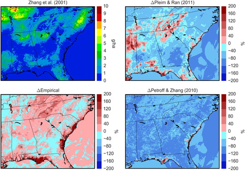
Fig. 13. Cumulative PM_2.5 NH₄⁺ dry deposition (g ha⁻¹) (June 14–28, 2013) for the base Zhang et al. (2001) simulation and percent differences from the base for each of the tested particle deposition algorithms.

During the simulation period over the southeast U. S., total (wet + dry) PM_2.5 deposition was dominated by wet deposition (see Tables 2 and 3). In the base Zhang et al. simulation, PM_2.5dry deposition accounted for only 14.6 % of total PM_2.5 deposition over the domain, with a similar fraction and overall total deposited in the Pleim and Ran simulation. In the Petroff and Zhang simulation, dry deposition accounted for only 4.4% of total PM_2.5 deposition, and total particle deposition decreased by 8.0% as compared to the base Zhang et al. simulation. For the empirical simulation, mean dry deposition over the domain increased to almost 24% of the total PM_2.5 deposition, and total particle deposition increased by 7.1%. If only forested grid cells are considered (Table 3), the results are qualitatively similar but with a larger overall impact. In particular, the empirical simulation produced a 20% increase in total PM_2.5 deposition to forested grid cells with one-third of the total deposited as dry deposition.

Table 2. Domain mean wet, dry and total PM_2.5 deposition (g ha⁻¹) for each simulation; for Wet and Dry depositions, values in parentheses are the fractions of each deposition type in the Total; for Total deposition, values in parentheses are the percentage differences in total PM_2.5 deposition with respect to the base Zhang et al. simulation.

Simulation	Wet (g/ha)	Dry (g/ha)	Total (g/ha)
Zhang et al. (2001)	477.7 (85.4%)	81.6 (14.6%)	559.3
Pleim and Ran (2011)	477.5 (85.6%)	80.6 (14.4%)	558.1 (−0.2%)
Petroff and Zhang (2010)	492.1 (95.6%)	22.5 (4.4%)	514.6 (−8.0%)
Empirical	459.8 (76.4%)	142.2 (23.6%)	602.0 (+7.1%)

Table 3. Mean wet, dry and total PM_2.5 deposition (g ha⁻¹) for forested grid cells only for each simulation; for Wet and Dry depositions, values in parentheses are the fractions of each deposition type in the Total; for Total deposition, values in parentheses are the percentage differences in total PM_2.5 deposition with respect to the base Zhang et al. simulation.

Simulation	Wet (g/ha)	Dry (g/ha)	Total (g/ha)
Zhang et al. (2001)	526.3 (83.6%)	103.6 (16.4%)	629.9
Pleim and Ran (2011)	524.1 (78.8%)	140.8 (21.2%)	664.9 (+5.6%)
Petroff and Zhang (2010)	541.9 (95.0%)	28.3 (5.0%)	570.2 (−9.5%)
Empirical	503.9 (66.7%)	251.6 (33.3%)	755.5 (+20%)

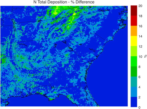
Figures 14 and 15 present the per cent increase in total deposition between the empirical simulation and the base Zhang et al. simulation for sulfur and nitrogen, respectively. As expected, the largest increases in total deposition occur over forested grid cells that received smaller wet deposition amounts. Because a larger fraction of sulfur deposition occurs in the particle phase than does nitrogen, larger increases are observed in total sulfur deposition (a maximum of 161% and domain mean of 7.5%) as compared to total nitrogen deposition (a maximum of 13% and domain mean of 1.3%). Since the southeast U. S. typically experiences frequent summer afternoon and evening rainfall, this result may underestimate the uncertainty in total deposition caused by the model-measurement discrepancy of particle deposition to forests. In particular, the western U. S. is normally far drier than the southeast and dry deposition of both sulfur and nitrogen accounts for a much larger fraction of total deposition there (NADP, 2016).

Fig. 14. Per cent increase in total sulfur deposition (all forms of sulfur in both dry and wet deposition) between the empirical simulation and the base Zhang et al. simulation. Maximum increase = 160.6%; Domain mean increase = 7.5%.

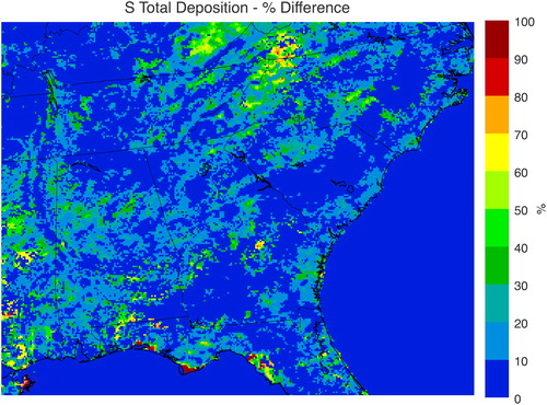
Fig. 15. Percent increase in total nitrogen deposition (all forms of nitrogen in both dry and wet deposition) between the empirical simulation and the base Zhang et al. simulation. Maximum increase = 13.0%; Domain mean increase = 1.3%.

Unfortunately, there are no model-independent measurements of particle deposition available with which to evaluate the results obtained here. Estimates of particle dry deposition from the USEPA’s Clean Air Status and Trends Network (CASTNET) are calculated using the method of Bowker et al. (2011) using deposition velocities calculated by the Multi-Layer Model of Meyers et al. (1998). The resulting inferential deposition estimates, which are combinations of model-generated deposition velocities and 7-day average PM_2.5 concentrations, are not ideal for comparison to 3D model predicted dry deposition. Nevertheless, Table 4 (and Figs. S-26 through S-28) presents mean biases and normalised mean biases for model predicted particle deposition (g ha⁻¹) vs. CASTNET estimated deposition for SO₄²⁻, NO₃⁻ and NH₄⁺, while Table 5 (and Figs. S-29 through S-31) presents similar statistics for PM_2.5 concentrations (µg m⁻³) of these species from CASTNET. Although the model vs. measurement comparisons of species surface concentrations suggest decreased biases when using the Empirical algorithm as compared to the Zhang et al. (2001) algorithm, a similar conclusion cannot be made for the model-dependent dry deposition comparisons.

Table 4. Mean bias (g ha⁻¹) and normalised mean bias (%) for model simulation vs CASTNet estimated PM_2.5 species dry deposition from filter samples obtained June 18–25, 2013 (N = 15). Model depositions accumulated to correspond to the CASTNet filter samples over the one-week time period (https://www.epa.gov/castnet).

Simulation	SO4^2=	NO3^−	NH4^+
Zhang et al. (2001)	+1.85 (+10.7%)	−0.75 (−42.3%)	+2.99 (+52.8%)
Pleim and Ran (2011)	+6.54 (+37.9%)	−1.13 (−63.6%)	+5.15 (+91.0%)
Petroff and Zhang (2010)	−10.1 (−58.3%)	−1.52 (−85.9%)	−3.70 (−65.5%)
Empirical	+26.1 (+ 151%)	−0.42 (−23.8%)	+7.61 (+135%)

Table 5. Mean bias (µg m⁻³) and normalised mean bias (%) for model simulation vs CASTNet PM_2.5 species concentrations from filter samples obtained June 18–25, 2013 (N = 15). Model concentrations averaged to correspond to the CASTNet filter samples over the 1-week time period (https://www.epa.gov/castnet).

Simulation	SO4^2=	NO3^−	NH4^+
Zhang et al. (2001)	+1.26 (+56.0%)	+0.06 (+27.7%)	+0.59 (+79.5%)
Pleim and Ran (2011)	+1.27 (+56.5%)	+0.08 (+33.6%)	+0.60 (+81.5%)
Petroff and Zhang (2010)	+1.45 (+64.5%)	+0.08 (+35.5%)	+0.67 (+91.3%)
Empirical	+0.94 (+41.8%)	+0.06 (+25.5%)	+0.48 (+65.5%)

4. Conclusions, implications and recommendations

Particle deposition algorithms used in most current air quality and atmospheric chemistry models have their origin in the work of Slinn (1982), Slinn and Slinn (1980) and Slinn (1977), which were based on measurements (a large fraction of which were wind-tunnel based) made in the 1970–80’s and earlier with technology available at that time. Nevertheless, as was shown, V_d(D_p) algorithms derived from the Slinn formulation can have substantial variation in predictions for identical environmental conditions and land use types. Moreover, comparisons of algorithm predictions of V_d generally do not agree very well with available measurements, especially for forested surface types, where the algorithms underpredict V_d by up to two orders of magnitude for particles in the diameter range 0.2–2.0 µm.

In this work, we have conducted a sensitivity study to estimate how uncertainties in particle deposition algorithms, as expressed by variations in V_d predictions among different commonly used algorithms and by model-measurement discrepancies, may impact surface PM_2.5 concentration distributions, total particle deposition and total (wet + dry) deposition. In this study, CAMx air quality model simulations were performed using three different but commonly used V_d(D_p) algorithms and an additional simulation was performed using an empirically based V_d(D_p) algorithm which better matches V_d measurements made over forested landscapes.

Surface PM_2.5 concentrations in the simulations were seen to differ by a few per cent between the algorithms, with the largest differences occurring between the Petroff and Zhang and empirical simulations. However, these results may be underestimated since boundary conditions for PM_2.5 for the SENEX domain did not change between the simulations and may be modulating a larger effect on surface concentrations that would be seen if the domain extended over a larger area. The largest effect of differences in V_d(D_p) algorithms in the simulations was on PM_2.5 deposition. Depending upon the choice of algorithm, estimated domain mean total PM_2.5 deposition differed by as much as 17% between simulations (Empirical vs. Petroff & Zhang), while PM_2.5dry deposition for individual forested grid cells differed by >200 %.

The empirically-based simulation over the heavily forested Southeast US predicted a domain mean increase in total PM_2.5 deposition of 7% and a 20% increase in total PM_2.5 deposition averaged over all forested grid cells. Further, total (wet + dry) sulfur deposition increased by a maximum of 161% and a domain mean value of 7.5%, while total nitrogen deposition increased by a maximum of 13% and a domain mean of 1.3%. These results suggest that if field measurements of particle deposition velocities over forests are correct, and current state-of-the-science models underestimate accumulation mode particle deposition, then model-based estimates of total deposition may be underestimated, especially over forested landscapes in the dry western US. This underestimation of particle deposition and total deposition to forested landscapes may be significant for regulations based on the critical loads concept.

In this study, we have focussed on uncertainties in particle deposition only as a function of differences in predictions from V_d(D_p) algorithms commonly used in air quality and atmospheric chemistry models and from differences between the algorithms and V_d measurements over various land use types. In fact, there are other uncertainties inherent in particle dry deposition modelling that are not accounted for in current state-of-the-science air quality and atmospheric chemistry models. One of these is the fact that most size-resolved field measurements of particle deposition velocity record not only downward fluxes of particles (i.e. deposition), but a large fraction of the time upward fluxes (resuspension or emission) are measured as well. This phenomenon was noted as far back as the 1980’s (Hicks et al., 1982; 1989) and is observed routinely with more modern instruments and technologies (e.g. Vong et al., 2010; Gordon et al., 2011) and has been examined theoretically by Pryor et al. (2008b). However, since in-canopy physical and chemical processes are largely ignored by current air quality and atmospheric chemistry models (Saylor and Hicks, 2016), there are no mechanisms included in these models that can produce upward particle fluxes. In these models, only particle deposition to vegetative canopies is allowed to occur, not in-canopy particle production and emission. Another uncertainty in modern air quality and atmospheric chemistry models relates to the fact that dry deposition is not a spatially ergodic process, meaning that a measurement made at one location under one set of conditions may not necessarily be representative of another (similar) location and set of conditions (Hicks, 1995). Since the nature of a surface on which a gas or particle is dry depositing is often such a controlling factor in the rate at which it deposits, simulating dry deposition over a single multi-kilometer wide grid cell, which may in reality be a complex patchwork of multiple land use categories, is fraught with uncertainty. How does one interpret a dry deposition flux calculated for such a grid cell as part of a total deposition estimate, when the actual deposition to a forest-covered sensitive ecosystem in that grid cell may be 10× or larger than a nearby plowed field? Additional uncertainties related to the heterogeneity of grid cell depositing surfaces are those of edge effects (Hicks, 1995) and complex terrain (Hicks, 2008), both of which are estimated to result in larger dry deposition rates than are simulated by current air quality and atmospheric chemistry models. In sum, the uncertainties in the current state of dry deposition science and its modelling clearly lead to uncertainties in the current application of large-scale models to derive estimates of total deposition.

The results from this exercise in model sensitivity and uncertainty cannot be definitively evaluated because of the lack of suitable particle deposition measurements during the simulation period, but the results strongly indicate that more attention needs to be paid to the uncertainties identified here. Any estimates of particle dry deposition derived from model simulations contain substantial uncertainties and potential underestimates that will affect calculations of total deposition for critical load assessments, and these uncertainties will vary across land use types and local micrometeorological conditions. New measurement technologies and the improved accuracy of older technologies now allow the potential for the deposition measurement and modelling communities to revisit old assumptions and fashion new (or improved versions of the old) theories and algorithms of the particle dry deposition process. Since accurate predictions of atmospheric particle concentrations and deposition are critically important for future air quality, weather and climate models and assessment and management of pollutant deposition to sensitive ecosystems, an investment in new dry deposition measurements in conjunction with integrated modelling efforts seems not only justified but vitally necessary to advance and improve the treatment of these processes in the models.

Supplemental data

Supplemental data for this article can be accessed here.

Acknowledgements

The research was supported in part by NOAA’s U. S. Weather Research Program (RDS). One author (BBB) was supported through a National Research Council Research Associate Fellowship. The authors gratefully acknowledge Dr. Alexandre Petroff for providing the code for his particle deposition algorithm and Dr. Mark Cohen (NOAA Air Resources Laboratory) for valuable feedback on the manuscript.

Disclosure statement

No potential conflict of interest was reported by the authors.

References

- Ahlm, L., Krejci, R., Nilsson, E. D., Martensson, E. M., Vogt, M. and co-authors. 2010. Emission and dry deposition of accumulation mode particles in the Amazon Basin. Atmos. Chem. Phys. 10, 10237–10253. doi:10.5194/acp-10-10237-2010.
- Allen, A. G., Harrison, R. M. and Nicholson, K. W. 1991. Dry deposition of fine aerosol to a short grass surface. Atmos. Environ. 25A, 2671–2676.
- Baumgardner, R. E. Jr, Lavery, T. F., Rogers, C. M. and Isil, S. S. 2002. Estimates of the atmospheric deposition of sulfur and nitrogen species: Clean Air Status and Trends Network, 1990-2000. Environ. Sci. Technol. 36, 2614–2629. doi:10.1021/es011146g.
- Beswick, K. M., Hargreaves, K. J., Gallagher, M. W., Choularton, T. W. and Fowler, D. 1991. Size-resolved measurements of cloud droplet deposition velocity to a forest canopy using an eddy correlation technique. Q. J. R. Met. Soc. 117, 623–645. doi:10.1002/qj.49711749910.
- Bowker, G. E., Schwede, D. B., Lear, G. G., Warren-Hicks, W. J. and Finkelstein, P. L. 2011. Quality assurance decisions with air models: A case study of imputation of missing input data using EPA’s Multi-Layer Model. Water Air Soil Pollut. 223, 391–402.
- Brook, J. R., Di-Giovanni, F., Cakmak, S. and Meyers, T. P. 1997. Estimation of dry deposition velocity using inferential models and site-specific meteorology – uncertainty due to siting of meteorological towers. Atmos. Environ. 31, 3911–3919. doi:10.1016/S1352-2310(97)00247-1.
- Buzorius, G., Rannik, U., Makela, J. M., Keronen, P., Vesala, T. and co-authors. 2000. Vertical aerosol fluxes measured by the eddy covariance method and deposition of nucleation mode particles above a Scots pine forest in southern Finland. J. Geophys. Res. 105, 19905–19916.
- Byun, D. and Schere, K. 2006. Review of the governing equations, computational algorithms, and other components of the Models-3 Community Multiscale Air Quality (CMAQ) modeling system. Appl. Mech. Rev. 59, 51–77. doi:10.1115/1.2128636.
- Caffrey, P. F., Ondov, J. M., Zufall, M. J. and Davidson, C. I. 1998. Determination of size-dependent dry particle deposition velocities with multiple intrinsic elemental tracers. Environ. Sci. Technol. 32, 1615–1622. doi:10.1021/es970644f.
- Chamberlain, A. C. 1967. Transport of Lycopodium spores and other small particles to rough surfaces. Proceedings of the Royal Society of London 296A, 45–70.
- Clough, W. S. 1975. The deposition of particles on moss and grass surfaces. Atmos. Environ. 9, 1113–1119. doi:10.1016/0004-6981(75)90187-0.
- Contini, D., Donateo, A., Belosi, F., Grasso, F. M., Santachiara, G. and co-authors. 2010. Deposition velocity of ultrafine particles measured with the eddy correlation method over the Nansen Ice Sheet (Antarctica). J. Geophys. Res. 115, D16202. doi:10.1029/2009JD013600.
- Deardorff, J. W. 1970. Convective velocity and temperature scales for the unstable planetary boundary layer and for Rayleigh convection. J. Atmos. Sci. 27, 1211–1213.
- Driscoll, C. T., Lawrence, G. B., Bulger, A. J., Butler, T. J., Cronan, C. S. and co-authors. 2001. Acidic deposition in the northeastern United States: sources and inputs, ecosystem effects, and management strategies. Biogeoscience 51, 180–198.
- Duan, B., Fairall, C. W. and Thomson, D. W. 1988. Eddy correlation measurements of the dry deposition of particles in wintertime. J. Appl. Meteor. 27, 642–652.
- Ellis, R. A., Jacob, D. J., Sulprizio, M. P., Zhang, L., Holmes, C. D. and co-authors. 2013. Present and future nitrogen deposition to national parks in the United States: critical load exceedances. Atmos. Chem. Phys. 13, 9083–9095.
- Environ International Corporation. 2012. CAMx: User’s Guide Comprehensive Air Quality Model with Extensions, Version 6.0, Novato, California. (http:/www.environcorp.com).
- Gallagher, M. W., Choularton, T. W., Morse, A. P. and Fowler, D. 1988. Measurements of the size dependence of cloud droplet deposition at a hill site. Q. J. R. Meteorol. Soc. 114, 1291–1303.
- Gallagher, M. W., Beswick, K. M., Duyzer, J., Westrate, H., Choularton, T. W. and co-authors. 1997. Measurements of aerosol fluxes to Speulder Forest using a micrometeorological technique. Atmos. Environ. 31, 359–373.
- Galloway, J. N., Aber, J. D., Erisman, J. W., Seitzinger, S. P., Howarth, R. W. and co-authors. 2003. The nitrogen cascade. Bioscience 53, 341–356.
- Gaman, A., Rannik, U., Aalto, P., Pohja, T., Siivola, E. and co-authors. 2004. Relaxed eddy accumulation system for size resolved aerosol particle flux measurements. J. Atmos. Oceanic Technol. 21, 933–943.
- Gong, W., Makar, P. A., Zhang, J., Milbrandt, J., Gravel, S. and co-authors. 2015. Modelling aerosol-cloud-meteorology interaction: A case study with a fully coupled air quality model (GEM-MACH). Atmos. Environ. 115, 695–715.
- Gordon, M., Staebler, R. M., Liggio, J., Vlasenko, A., Li, S.-M. and co-authors. 2011. Aerosol flux measurements above a mixed forest at Borden, Ontario. Atmos. Chem. Phys. 11, 6773–6786.
- Grell, G. and Baklanov, A. 2011. Integrated modeling for forecasting weather and air quality: A call for fully coupled approaches. Atmos. Environ. 45, 6845–6851.
- Gronholm, T., Aalto, P. P., Hiltunen, V., Rannik, U., Rinne, J. and co-authors. 2007. Measurements of aerosol particle dry deposition velocity using the relaxed eddy accumulation technique. Tellus 59B, 381–386.
- Gronholm, T., Launiainen, S., Ahlm, L., Martensson, E. M., Kulmala, M. and co-authors. 2009. Aerosol particle dry deposition to canopy and forest floor measured by two-layer eddy covariance system. J. Geophys. Res. 114, D04202. doi:10.1029/2008JD010663.
- Grosch, S. and Schmitt, G. 1988. Experimental Investigations on the Deposition of Trace Elements in Forest Area. In: Environmental Meteorology (eds. K. Grefen and L. Lobel). Kluwer Academic Publishers, Dordrecht, The Netherlands, pp. 201–216.
- Held, A., Orsini, D. A., Vaattovaara, P., Tjernstrom, M. and Leck, C. 2011a. Near-surface profiles of aerosol number and concentration and temperature over the Arctic Ocean. Atmos. Meas. Tech. 4, 1603–1616.
- Held, A., Brooks, I. M., Leck, C. and Tjernstrom, M. 2011b. On the potential contribution of open lead particle emissions to the central Arctic aerosol concentration. Atmos. Chem. Phys. 11, 3093–3105.
- Hettelingh, J.-P., Posch, M., De Smet, P. and Downing, R. J. 1995. The use of critical loads in emission reduction agreements in Europe. Water Air Soil Pollut. 85, 2381–2388.
- Hicks, B. B., Saylor, R. D. and Baker, B. D. 2016. Dry deposition of particles to canopies – A look back and the road forward. J. Geophys. Res. – Atmos. 121, 14691–14707. doi:10.1002/2015JD024742.
- Hicks, B. B., Wesely, M. L., Durham, J. L. and Brown, M. A. 1982. Some direct measurements of atmospheric sulfur fluxes over a pine plantation. Atmos. Environ. 16, 2899–2903.
- Hicks, B. B., Matt, D. R., McMillen, R. T., Womack, J. D., Wesely, M. L. and co-authors. 1989. A field investigation of sulfate fluxes to a deciduous forest. J. Geophys. Res. 94, 13003–13011.
- Hicks, B. B. 1986. Measuring dry deposition: a re-assessment of the state of the art. Water Air Soil Pollut. 30, 75–90.
- Hicks, B. B. 1995. On the determination of total deposition to remote areas. Stud. Environ. Sci. 64, 163–173.
- Hicks, B. B. 2008. On estimating dry deposition rates in complex terrain. J. Appl. Meteor. Climatol. 47, 1651–1658.
- Hofken, K. D. and Gravenhorst, G. 1982. Deposition of atmospheric aerosol particles to beech- and spruce forest. In: Deposition of Atmospheric Pollutants (eds. H. W. Georggi and J. Pankrath). D. Reidel Publishing Company, Oberursel/Taunus, Germany, pp. 191–194.
- Houyoux, M. R. and Vukovich, J. M. 1999. Updates to the Sparse Matrix Operator Kernel Emissions (SMOKE) Modeling System and Integration with Models-3. In: Proceedings of the Emission Inventory: Regional Strategies for the Future. Raleigh, NC, Air and Waste Management Association Annual Meeting, pp. 430–440.
- Hummelshoj, P. 1994. Dry Deposition of Particles and Gases. PhD Thesis, Technical University of Denmark.
- Ibrahim, M., Barrie, L. A. and Fanaki, F. 1983. An experimental and theoretical investigation of the dry deposition of particles to snow, pine trees and artificial collectors. Atmos. Environ. 17, 781–788.
- Im, U., Bianconi, R., Solazzo, E., Kioutsioukis, I., Badia, A., and co-authors. 2015. Evaluation of operational online-coupled regional air quality models over Europe and North America in the context of AQMEII phase 2. Part II: Particular matter. Atmos. Environ. 115, 421–441.
- IPCC 2014. Climate Change 2014: Synthesis Report. Contribution of Working Groups I, II, and III to the Fifth Assessment Report of the Intergovernmental Panel on Climate Change (Core Writing Team, eds., R. K. Pachauri and L. A. Meyer), IPCC, Geneva, Switzerland, 151 pp.
- Katul, G. G., Gronholm, T., Launiainen, S. and Vesala, T. 2011. The effects of the canopy medium on dry deposition velocities of aerosol particles in the canopy sub-layer above forested ecosystems. Atmos. Environ. 45, 1203–1212.
- Koo, B., Ansari, A. S. and Pandis, S. N. 2003. Integrated approaches to modeling the organic and inorganic atmospheric aerosol components. Atmos. Environ. 37, 4757–4768.
- Larkin, N. K., O'Neill, S. M., Solomon, R., Raffuse, S., Strand, T., and co-authors. 2009. The BlueSky smoke modeling framework. Int. J. Wildland Fire 18, 906–920.
- Lavi, A., Farmer, D. K., Segre, E., Moise, T., Rotenberg, E. and co-authors. 2013. Fluxes of fine particles over a semi-arid pine forest: Possible effects of a complex terrain. Aerosol. Sci. Technol. 47, 906–915.
- Lee, P., McQueen, J., Stajner, I., Huang, J., Pan, L., and co-authors. 2017. NAQFC developmental forecast guidance for fine particulate matter (PM2.5). Weather Forecast. 32, 343–360. doi:10.1175/WAF-D-15-0163.1.
- Liu, S., Lu, L., Mao, D. and Jia, L. 2007. Evaluating parameterizations of aerodynamic resistance to heat transfer using field measurements. Hydrol. Earth Syst. Sci. 11, 769–783.
- Lorenz, R. and Murphy, C. E. Jr.1989. Dry deposition of particles to a pine plantation. Boundary-Layer Meteorol. 46, 355–366.
- Mammarella, I., Rannik, U., Aalto, P., Keronen, P., Vesala, T. and co-authors. 2011. Long-term aerosol particle flux observations. Part II: Particle size statistics and deposition velocities. Atmos. Environ. 45, 3794–3805.
- Matsuda, K., Fujimura, Y., Hayashi, K., Takahashi, A. and Nakaya, K. 2010. Deposition velocity of PM2.5 sulfate in the summer above a deciduous forest in central Japan. Atmos. Environ. 44, 4582–4587.
- Matsuda, K., Watanabe, I., Mizukami, K., Ban, S. and Takahashi, A. 2015. Dry deposition of PM2.5 sulfate above a hilly forest using relaxed eddy accumulation. Atmos. Environ. 107, 255–261.
- Meyers, T. P., Finkelstein, P., Clarke, J., Ellestad, T. G. and Sims, P. F. 1998. A multilayer model for inferring dry deposition using standard meteorological measurements. J. Geophys. Res. 103, 22,645–22,661.
- Moller, U. and Schumann, G. 1970. Mechanisms of transport from the atmosphere to the Earth’s surface. J. Geophys. Res. 75, 3013–3019.
- Morris, R., Koo, B. and Yarwood, G. 2005. Evaluation of multisectional and two-section particulate matter photochemical grid models in the western United States. J. Air Waste Manag. Assoc. 55, 1683–1693.
- National Atmospheric Deposition Program 2016. Total Deposition 2015 Annual Map Summary. NADP Data Report 2016-02. Illinois State Water Survey, University of Illinois at Urbana-Champaign.
- Nemitz, E., Gallagher, M. W., Duyzer, J. H. and Fowler, D. 2002. Micrometeorological measurements of particle deposition velocities to moorland vegetation. Q. J. R. Meteorol. Soc. 128, 2281–2300.
- Nenes, A., Pilinis, C. and Pandis, S. N. 1998. ISORROPIA: A new thermodynamic model for multiphase multicomponent inorganic aerosols. Aquatic Geochem. 4, 123–152.
- Nenes, A., Pilinis, C. and Pandis, S. N. 1999. Continued development and testing of a new thermodynamic aerosol module for urban and regional air quality models. Atmos. Environ. 33, 1553–1560.
- Neumann, H. H. and den Hartog, G. 1985. Eddy correlation measurements of atmospheric fluxes of ozone, sulphur, and particulates during the Champaign Intercomparison Study. J. Geophys. Res. 90, 2097–2110.
- Nilsson, E. D. and Rannik, U. 2001. Turbulent aerosol fluxes over the Arctic Ocean, 1. Dry deposition over sea and pack ice. J. Geophys. Res. 106, 32,125–32,137.
- O’Neill, S. M., N. K., Larkin, J., Hoadley, G., Mills, J. K., Vaughan, R. and co-authors. 2009.,. Regional real-time smoke prediction systems. In: Wildland Fires and Air Pollution: Developments in Environmental Science, Vol. 8, (eds by A. Bytnerowicz. et al. ), Elsevier B.V., Oxford, U.K. pp 499–534.
- Ould-Dada, Z. 2002. Dry deposition profile of small particles within a model spruce canopy. Sci. Total Environ. 286, 83–96.
- Pan, L., Tong, D., Lee, P., Kim, H. and Chai, T. 2014. Assessment of NOx and O3 forecasting performances in the U.S. National Air Quality Forecasting Capability before and after the 2012 major emissions updates. Atmos. Environ. 95, 610–619. doi:10.1016/j.atmosenv.2014.06.020.
- Pardo, L. H., Fenn, M. E., Goodale, C. L., Geiser, L. H., Driscoll, C. T. and co-authors. 2011. Effects of nitrogen deposition and empirical nitrogen critical loads for ecoregions of the United States. Ecol. Appl. 21, 3049–3082.
- Petroff, A., Mailliat, A., Amielh, M. and Anselmet, F. 2008a. Aerosol dry deposition on vegetative canopies. Part I: Review of present knowledge. Atmos. Environ. 42, 3625–3653.
- Petroff, A., Mailliat, A., Amielh, M. and Anselmet, F. 2008b. Aerosol dry deposition on vegetative canopies. Part II: A new modelling approach and applications. Atmos. Environ. 42, 3654–3683.
- Petroff, A., Zhang, L., Pryor, S. C. and Belot, Y. 2009. An extended dry deposition model for aerosols onto broadleaf canopies. Aerosol Sci. 40, 218–240.
- Petroff, A. and Zhang, L. 2010. Development and validation of a size-resolved particle dry deposition scheme for application in aerosol transport models. Geosci. Model Dev. 3, 753–769.
- Pilinis, C., Capaldo, K. P., Nenes, A. and Pandis, S. N. 2000. MADM – A new multicomponent aerosol dynamics model. Aerosol Sci. Technol. 32, 482–502.
- Pleim, J. 2007. A combined local and nonlocal closure model for the atmospheric boundary layer. Part I: Model description and testing. J. Appl. Meteorol. Climatol. 46, 1383–1395. doi:10.1175/JAM2539.1.
- Pleim, J. and Ran, L. 2011. Surface flux modeling for air quality applications. Atmosphere 2, 271–302.
- Pryor, S. C., Gallagher, M., Sievering, H., Larsen, S. E. and Barthelmie, R. and co-authors. 2008a. A review of measurement and modeling results of particle atmosphere-surface exchange. Tellus 60B, 42–75.
- Pryor, S. C., Barthelmie, R. J., Sorensen, L. L., Larsen, E., Sempreviva, A. M. and co-authors. 2008b. Upward fluxes of particles over forests: when, where, why? Tellus 60B, 372–380.
- Pryor, S. C. 2006. Size-resolved particle deposition velocities of sub-100 nm diameter particles over a forest. Atmos. Environ. 40, 6192–6200.
- Pryor, S. C., Larsen, S. E., Sorensen, L. L., Barthelmie, R. J., Gronholm, T. and co-authors. 2007. Particle fluxes over forests: Analyses of flux methods and functional dependencies. J. Geophys. Res. 112, D07205. doi:10.1029/2006JD008066.
- Pryor, S. C., Barthelmie, R. J., Spaulding, A. M., Larsen, S. E. and Petroff, A. 2009. Size-resolved fluxes of sub-100-nm particles over forests. J. Geophys. Res. 114, D18212. doi:10.1029/2009JD012248.
- Pye, H. O. T., Liao, H., Wu, S., Mickley, L. J., Jacob, D. J. and co-authors. 2009. Effect of changes in climate and emissions on future sulfate-nitrate-ammonium aerosol levels in the United States. J. Geophys. Res. 114, D01205. doi: 10.1029/2008JD010701.
- Ruminski, M., Kondragunta, S., Draxler, R. and Zeng, J. 2006. Recent Change to the Hazard Mapping System. Preprint: 15th International Emission Inventory Conf.: Reinventing Inventories – New Ideas in New Orleans. New Orleans, LA, May 15-18, 2006. http://www.epa.gov/ttn/chief/conference/ei15/session10/ruminski.pdf (last accessed Nov 20, 2014).
- Saide, P. E., Spak, S. N., Pierce, R. B., Pierce, Otkin, J. A., Schaack, T. K. and co-authors. 2015. Central American biomass burning smoke can increase tornado severity in the U. S. Geophys. Res. Lett. 42, 956–965. doi:10.1002/2014GL062826.
- Saide, P. E., Thompson, G., Eidhammer, T., da Silva, A. M., Pierce, R. B. and co-authors. 2016. Assessment of biomass burning smoke influence on environmental conditions for multiyear tornado outbreaks by combining aerosol-aware microphysics and fire emission constraints. J. Geophys. Res. Atmos. 121, 10,294–10,311. doi:10.1002/2016JD025056.
- Sarwar, G., Luecken, D., Yarwood, G., Whitten, G. and Carter, W. 2008. Impact of an updated carbon bond mechanism on predictions from the CMAQ modeling system: Preliminary assessment. J. Appl. Meteor. Climatol. 47, 3–14. doi:10.1175/2007JAMC1393.1.
- Saylor, R. D. and Hicks, B. B. 2016. New directions: Time for a new approach to modeling surface-atmosphere exchanges in air quality models? Atmos. Environ. 129, 229–233.
- Schwede, D. B. and Lear, G. G. 2014. A novel hybrid approach for estimating total deposition in the United States. Atmos. Environ. 92, 207–220.
- Sievering, H. 1981. Profile measurements of particle mass transfer at the air-water interface. Atmos. Environ. 15, 123–129.
- Sievering, H. 1982. Profile measurements of particle dry deposition velocity at an air-land interface. Atmos. Environ. 16, 301–306.
- Sievering, H. 1988. Small-particle dry deposition measurements: A comparison of gradient and eddy flux techniques over agricultural fields, In: Annual Meeting of Air Pollution Control Association, Dallas, Texas, June 19–24, 6, pp. 88–101.
- Slinn, W. G. N. 1982. Predictions for particle deposition to vegetative canopies. Atmos. Environ. 16, 1785–1794.
- Slinn, W. G. N. 1977. Some approximations for the wet and dry removal of particles and gases from the atmosphere. Water Air Soil Pollut. 7, 513–543.
- Slinn, S. A. and Slinn, W. G. N. 1980. Predictions for particle deposition on natural waters. Atmos. Environ. 14, 1013–1016.
- Solazzo, E., Bianconi, R., Pirovano, G., Matthias, V., Vautard, R., and co-authors. 2012. Operational model evaluation for particulate matter in Europe and North America in the context of AQMEII. Atmos. Environ. 53, 75–92.
- Sun, F., Yin, Z., Lun, X., Zhao, Y., Li, R. and co-authors. 2014. Deposition velocity of PM2.5 in the winter and spring above deciduous and coniferous forests in Beijing, China. PLoS One 9, e97723. doi: 10.1371/journal.pone.0097723.
- Tong, D. Q., Lamsal, L., Pan, L., Ding, C., Kim, H. and co-authors. 2015. Long-term NOx trends over large cities in the United States during the great recession: Comparison of satellite retrievals, ground observations, and emission inventories. Atmos. Environ. 107, 70–84.
- U. S. Forest Service, National Park Service, U. S. Fish and Wildlife Service. 2011. Federal Land Managers’ Interagency Guidance for Nitrogen and Sulfur Deposition Analyses: November 2011 (Natural Resource Report, National Park Service, Denver, Colorado).
- Vong, R. J., Vong, I. J., Vickers, D. and Covert, D. S. 2010. Size-dependent aerosol deposition velocities during BEARPEX’07. Atmos. Chem. Phys. 10, 5749–5758.
- Vong, R. J., Vickers, D. and Covert, D. S. 2004. Eddy correlation measurements of aerosol deposition to grass. Tellus 56B, 105–117.
- Waraghai, A. and Gravenhorst, G. 1989. Dry deposition of atmospheric particles to an old spruce stand, in: Mechanisms and Effects of Pollutant Transfer into Forests. (ed. H. W. Georgii), Kluwer Academic Publishers, London, pp. 77–86.
- Wesely, M. L., Hicks, B. B., Dannevik, W. P., Frisella, S. and Husar, R. B. 1977. An eddy-correlation measurement of particulate deposition from the atmosphere. Atmos. Environ. 11, 561–563.
- Wesely, M. L., Cook, D. R., Hart, R. L. and Speer, R. E. 1985. Measurements and parameterization of particulate sulfur dry deposition over grass. J. Geophys. Res. 90, 2131–2143.
- Wyers, G. P. and Duyzer, J. H. 1997. Micrometeorological measurement of the dry deposition flux of sulphate and nitrate aerosols to coniferous forest. Atmos. Environ. 31, 333–343.
- Zhang, L., Gong, S., Padro, J. and Barrie, L. 2001. A size-segregated particle dry deposition scheme for an atmospheric aerosol module. Atmos. Environ. 35, 549–560.
- Zhang, L. and Vet, R. 2006. A review of current knowledge concerning size-dependent aerosol removal. China Particuol. 4, 272–282.
- Zhang, J., Shao, Y. and Huang, N. 2014. Measurements of dust deposition velocity in a wind-tunnel experiment. Atmos. Chem. Phys. 14, 8869–8882.
- Zufall, M. J., Davidson, C. I., Caffrey, P. F. and Ondov, J. M. 1998. Airborne concentrations and dry deposition fluxes of particulate species to surrogate surfaces deployed in southern Lake Michigan. Environ. Sci. Technol. 32, 1623–1628.