The MACv2 aerosol climatology

Abstract

The MAC aerosol climatology defines monthly global maps for aerosol properties. The definition of mid-visible optical and microphysical properties is strongly linked to multi-year statistics of observations by sun-photometers of the AERONET and MAN ground networks. As available statistics are spatially sparse, context from bottom-up global modelling is added. Now in its second version, oceanic MAN reference data are included, a different lower anthropogenic fraction is assumed and the merging of the data-statistics is improved. Hereby, now only absolute properties are merged and trusted photometer data are given stronger weights via regional corrections in place of local domain limited corrections. Global average mid-visible (550 mn) aerosol properties are 0.12 for the aerosol optical depth (AOD), 0.94 for the single scattering albedo (SSA) and 0.7 for the asymmetry-factor (ASY). Averages for sub-micrometer (fine-mode) and super-micrometer (coarse-mode) aerosol sizes are 0.063 (AODf) and 0.058 (AODc), 0.92 (SSAf) and 0.965 (SSAc) and 0.64 (ASYf) and 0.77 (ASYc), respectively. A new element is the separation of aerosol absorption (AAOD) by sky-/sun-photometers into fine-mode and coarse-mode contributions. These properties as well as the fine-mode effective radii were merged with background data from global modelling yielding global averages of 0.0051 (AAODf), 0.0021 (AAODc) and 0.18 μm (RE,f). Local monthly mode detail now allows (in a ‘top-down’ approach) to extract global distributions for aerosol component amounts and sizes. As the considered components for soot (BC), organics (OC), non-absorbing fine-mode (SU), sea-salt (SS) and mineral dust (DU) have pre-defined spectrally resolved properties, optical properties at other than mid-visible wavelengths are automatically defined – as required in broadband radiative transfer applications. With component information (e.g. amount, composition and size) also MAC estimates for CCN and IN concentrations are possible and also a simple MAC based aerosol retrieval model for satellite sensor data is suggested.

Keywords:

• atmosphere
• aerosol
• optical
• radiative
• global

1. Introduction

Tropospheric aerosols originate from many sources of natural (e.g. windblown dust, sea-spray, wild-fires) or anthropogenic (e.g. fossil fuel burning, agricultural burning) origin. Since the aerosol lifetime is only on the order of a few days (mainly due to the removal by precipitation), tropospheric aerosols are highly variable in concentration and composition. However, only aerosol sizes larger than a tenth of a micrometer in size (>0.05 μm in radius) directly influence the radiative energy distribution in the atmosphere. Sub-micrometer (fine-mode) sizes only affect the solar radiative transfer, while super-micrometer (coarse-mode) sizes modulate both solar and terrestrial radiative energy distributions.

Although the influence of aerosols is small compared to that of clouds, there is from a climate change perspective a strong interest on the impact of aerosol, because part of today’s atmospheric aerosol is anthropogenic in nature. However, quantifying global aerosol radiative effects via model simulations is challenging (Kinne et al., 2003; Textor et al., 2007). In these ‘bottom-up’ approaches, emissions of different aerosol species and pre-cursor gases are chemically and cloud processed, mixed, transported and removed. In addition, assumptions about particle size, water uptake and component mixing are required to establish aerosol optical properties (which are the basis in the determination of associated aerosol radiative effects). With accuracy limitations to (emission) input, processing mechanisms in modelling and microphysical assumptions, these ‘bottom-up’ approaches have large uncertainties and are computer time intensive as well. Thus, there is a need for faster and more direct approaches to define characteristic aerosol optical properties – even on global scales.

Alternately, observations of solar attenuation and solar scattering directly offer data on aerosol properties. In particular, globally distributed sun-/sky photometer ground networks offer simultaneous data on the three most relevant aerosol properties for radiative transfer: on aerosol column amount and on column averages for aerosol size and for aerosol absorption. All three aerosol properties together inform in a ‘top-down’ approach on aerosol composition and even on aerosol mass.

Such an (observation-) data based ‘top-down’ approach is the topic of this contribution, which describes the second version of the Max-Planck Aerosol climatology (MACv2). Aerosol optical properties for aerosol amount and aerosol absorption, both as function of size-modes with associated effective radii, are provided in monthly climatologies with global (1 × 1 deg lat/lon) coverage. Limitations of older aerosol climatologies for aerosol optical properties (e.g. Köpke et al., 1997) in terms of spatial, vertical and temporal coverage, required assumptions to aerosol water uptake and failures to define the pre-industrial state were already addressed in the first version of the MAC climatology. MACv1 (Kinne et al., 2013) scaled observed aerosol optical property statistics with relative context by model-ensemble median data from 'bottom-up' modeling. MACv2 updates over MACv1 include more recent AERONET data and now also oceanic MAN reference data, a modified spatial merging procedure, a more solid (now component based) spectral extension and an update for anthropogenic AOD contributions.

In chapter 2, the MACv2 mid-visible optical column properties and their global properties are introduced. In chapter 3, choices for aerosol component types and sizes are defined and based on these definitions global distributions of component mixtures are suggested (where local monthly mixtures are consistent with the optical and microphysical properties of MACv2). Definitions for anthropogenic aerosol are covered in chapter 4. The spectral extension of the aerosol radiative properties (as needed for radiative transfer simulations) is presented in chapter 5 by combining the spectral information of the pre-defined components and their assigned local monthly mixtures. In chapter 6, the assumptions for the vertical distribution are explained. Chapter 7 offers estimates for aerosol concentrations and chapter 8 introduces a simple model for first guesses in satellite retrievals of aerosol amount, by offering likely local properties on needed assumption for absorption and size.

2. Mid-visible column properties

2.1. What is MAC?

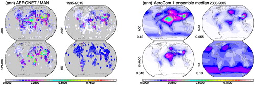
The Max Planck institute Aerosol climatology (MAC) is defined by monthly global (1 × 1 deg) fields for aerosol optical and microphysical properties. Central to these fields are atmospheric column aerosol optical properties in the mid-visible spectral region (at 550 nm). These column properties are based on trusted ground-based observations sampled over the last two decades. As observations are sparsely distributed, spatial context from global ‘bottom-up’ modelling is added to yield spatially and temporally complete fields. In a so called ‘merging process’, monthly maps defined by global modelling are adjusted according to monthly statistics by ground-based sun photometry. Contributing photometry data are quality assured direct solar attenuation and sky radiances samples of CIMEL instruments of the AERONET network (Holben et al., 1998, 2001) and solar attenuation samples by handheld MICROTOPS instruments of the Marine Aerosol Network, MAN (Smirnov et al., 2009, 2011). The maps from modelling are defined by local monthly median values of 14 different AeroCom (phase1) models (Kinne et al., 2006). For a flavour of applied aerosol data in the development of the MAC climatology, annual average maps for four important aerosol properties are compared in Fig. 1.

Fig. 1. Input data for MACv2. Shown are the multi-annual averages of aerosol optical properties at 550 nm based on local sun-photometer measurements by AERONET and MAN (left block, local data are enlarged for better viewing) and by the AeroCom ‘bottom-up’ modelling ensemble (right block). The four sub-panels in each block display the aerosol optical depth AOD (upper left), the absorption aerosol optical depth AAOD (lower left, multiplied by a factor 10), the fine-model aerosol optical depth AODf (upper right) and the fine-mode effective radius REf (lower right). As sun-photometers over oceans (of MAN) can only address AOD and AODf properties, data coverage over oceans for AAOD and REf is poor.

2.2. What has changed since MACv1?

Compared to the initial MACv1 version (Kinne at al., 2013) major upgrades are incorporated. In MACv2 (1) more recent AERONET data are included so that the central reference year shifted from year 2000 to year 2005, (2) MAN data over oceans are now considered, (3) a new regional data merging procedure is applied, (4) only absolute properties are merged (e.g. AAOD instead of SSA), (5) pre-defined aerosol types are utilized to assign local component mixtures for a more consistent spectral dependence and (6) a new (smaller) anthropogenic fraction is applied.

2.3. What trusted quality data are applied?

Solar attenuation measurements (simultaneously at different solar wavelengths by sun-photometry from the ground) offer at cloud-free conditions reliable data on aerosol amount and averages for aerosol size (distribution) and for aerosol absorption. Together these (three) aerosol properties even inform about aerosol compositional mixtures. Particular accurate are aerosol amount data, which are quantified by the aerosol optical depth (AOD). The AOD is the vertically normalized exponential decay coefficient of direct solar irradiance attributed to aerosol.

Sun-photometers sample AOD at different solar wavelengths. Both, the used AERONET level 2 version 2 data over land and the MAN level 2 data over oceans sample at 380, 440, 670 and 870 nm. The sampled AOD spectral dependence reveals information on the average aerosol particle size. In a simple approach (involving AOD data at just 2 different wavelengths) smaller particle domination is indicated by a larger Angstrom parameters (the negative slope in d(ln[AOD])/(d(ln[wavelength]) space). The more advanced SDA approach (involving AOD data at 4 more solar wavelengths) separates AOD contributions by sub-micrometer (fine-mode) and by super-micrometer (coarse-mode) sizes (O’Neill et al., 2003). Such a property separation by size-modes complements the size-representations in most aerosol schemes in global models (e.g. Kinne et al., 2006) and is therefore a preferred path to merge data on aerosol size. In addition to the direct solar intensity samples, the land-based AERONET data offer added information on solar spectral sky-radiances in near forward scattering and in side scattering directions. Via inverse radiative transfer methods (Dubovik et al., 2000) this added information provides estimates for average aerosol size distributions (for the 0.05 to 15 μm size range) and for average aerosol absorption estimates (via refractive index imaginary parts) at different wavelengths (at 440, 670, 870 and 1020 nm). Here, in the applied AERONET level 2 inversion data products the refractive index data information from level 1.5 data was reinstated.

2.3.1. Aerosol column amount

Direct solar attenuation (at cloud-free conditions) data define local monthly AOD. First sun-photometer AOD samples were interpolated (with the 440/870 Angstrom parameter) to the value at 550 nm (the reference wavelength in modelling and remote sensing). Then, multi-year (between 1995 and 2015) monthly local averages were established based on all quality checked AERONET version 2 and level 2 samples at more than 700 continental or island sites worldwide (https://aeronet.gsfc.nasa.gov/). And finally by applying site associated regional weights (Kinne et al., 2013) – local data were combined onto a 1 × 1 degree lat/lon spatial grid. Similarly interpolated, weighted (e.g. lower regional weights near coasts) and gridded were samples from almost 100 ship-cruises between 2006 and 2015 (https://aeronet.gsfc.nasa.gov/new_web/maritime_aerosol_network.html).

2.3.2. Aerosol column amount by size mode

The separating radius between the smaller fine-mode and larger coarse mode in MACv2 is set at 0.5 μm. From inversions applied to (AERONET sky-/sun samples), the concentrations of the 9 lower size bins (0.05 to 0.5 μm) contributed to the fine-mode AOD and the concentrations of the 13 larger size bins (0.5 to 15 μm) contributed to the coarse-mode AOD. In the absence of sky-radiance data (e.g. over oceans), fine-mode and coarse-mode AOD contributions (AODf, AODc) were estimated from AOD data at four or more solar wavelengths (O’Neill et al., 2003). The ratio between fine-mode AOD (AODf) and total AOD here is referred to as fine-mode fraction (FMF).

2.3.3. Aerosol column absorption

The imaginary part of the refractive index defines the aerosol absorption. The aerosol absorption is quantified by the Absorption Aerosol Optical Depth (AAOD). The AAOD is the other part of the AOD that is not associated with scattering. As the scattering potential is defined by the single scattering albedo (SSA = scattering-AOD/AOD) the absorption potential is defined by ([1-SSA] = AAOD/[AOD]). In the mid-visible spectral region, the SSA for atmospheric aerosol is on average at least an order of magnitude larger than the [1-SSA]. Thus, at lower aerosol loads the reduced sky scattering due to absorption is difficult to detect. As a consequence, only absorption data at larger aerosol loads (or AOD values) are more reliable (Dubovik et al., 2000). AERONET’s CIMEL sky-/sun-photometer samples offer refractive indices. But in their version 2 level 2 data all absorption data are removed for all AOD440nm < 0.4 cases, which is too conservative (Dubovik, private communication). Thus for MACv2 processing, the absorption data were considered reliable down to a lower AOD threshold (AOD at 550 nm > 0.2) and the removed refractive indices in the AERONET level 2 data were recovered from the level 1.5 data. For all absorption values below the 0.2 AOD threshold - based on local monthly statistics - the absorption potential [1 – SSA] at that threshold was prescribed. And for sites and months, when the AOD threshold was never reached, then the absorption potential [1 – SSA] of the statistically largest AOD values, locally were prescribed for all lower AOD cases. This method assured that the high uncertainty for absorption at low aerosol loads was reduced without biasing the sample statistics.

2.3.4. Aerosol column absorption by size-mode

A new element in MACv2 is the separation of the AAOD into fine-mode and coarse-mode contribution (AAODf, AAODc). The estimate for the fine-mode AAOD is based on an analysis of seasonal AERONET data over western African sites. In that region, both fine-mode (wildfire) and coarse mode (dust) contribute with significant absorption – with stronger fine-mode AAOD contributions from Nov to Feb and stronger coarse-mode AAOD contributions from Apr to Sep. The spectral dependence of the refractive index imaginary data (offered by AERONET sun-/sky inversion data) alone was not sufficient to separate the AAOD by size. However, with added information of the AOD fine mode fraction (FMF = AODf/AOD), estimates for the fine-mode absorption (AAODf) were possible (using western Africa data) via the following empirical relationship.

Table

AAODf,550 = AAOD,550 *FMF**(A*B/C) with	FMF= AODf,550/AOD,550
AAODc,550 = AAOD,550 – AAODf,550	A = 0.2 + 0.25*(1 – FMF)**2,
	B = ln(AAOD,440/AAOD,670)/ln(.67/.44)
	C = min (ln(AAOD,670/AAOD,1020)/ln(1.02/.67), B)

And once AAODf is extracted from the total AAOD, then also AAODc is automatically defined. Note, that AAODc is strongly affected by size, with significant contributions from larger mineral dust particles.

2.3.5. Aerosol column effective radius

The relevance of aerosol size is already addressed, as amount and absorption of aerosol is (see above) are already split into contributions by sub-micrometer (fine-mode) aerosol and super-micrometer (coarse-mode) sizes. In addition, from (to CIMEL sky-/sun samples) applied inversions, size distribution data define effective radii (RE = Σr**3}/{Σr**2) for both the fine-mode (REf) and for the coarse mode (REc). REf is an important parameter to estimate the aerosol number concentrations of optically detectable sizes (radii > 0.05 μm) and REf is essential for CCN estimates with MACv2 data (at low supersaturations).

2.4. How are data merged?

The merging combines the accuracy of local photometer statistics with gap-filling spatial context by global modelling using monthly statistics at 1 × 1 deg lat/lon spatially resolution. Then, global sub-regions with sufficient photometer sites are picked as illustrated in Fig. 2. In each of those regions, for each month interquartile averages of only matching grid-points are compared. Their ratio (photometer to modelling data) defines multipliers that are applied to all modelling background values in that region (and month). Finally, spatial inconsistencies of multipliers at regional boundaries are smoothed, by replacing local multipliers with +/– 6 deg in longitude and +/– 3 deg in latitude averages For an illustration derived annual average multipliers for properties of Fig. 1 (AOD, 10*AAOD, AODf and REf) are presented without and with boundary smoothing in Fig. 2.

Fig. 2. AERONET/MAN observation suggested (factor-1) changes to background data from modelling for the four properties of Fig. 1 – by region. Red colours indicate the need to increase model properties (with 1 referring to a doubling), blue colours require a reduction (with –1 referring to half the value) and grey colours indicate no changes due to a lack in reference data. Presented are for the four properties of Fig. 1 (of AOD, 10*AAOD, AODf and REf) annual average adjustments for the selected 21 regions before (left block) and after after (+/– 6 deg lon, +/–3 deg lat) smoothing (right block). Smoothed changes are applied to create MCv2 maps. Values below the labels are adjustment averages.

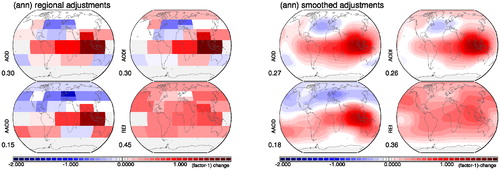
The applied smoothed adjustments (to the AeroCom phase 1 modelling background of Fig. 1) to yield the core MACv2 properties of Fig. 3.

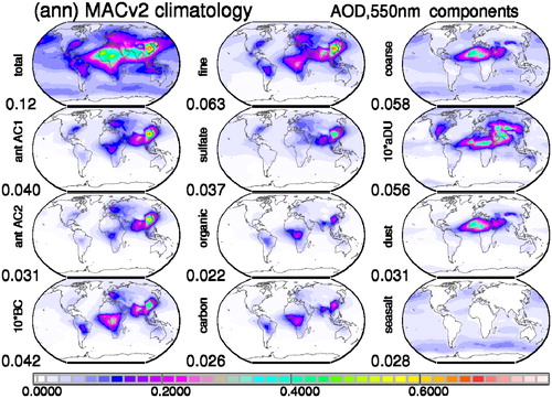
Fig. 3. Annual average maps of the MACv2 aerosol climatology. Global distributions (as result of the data-merging) are presented (left block) for the mid-visible AOD (column amount), for the mid-visible AAOD (column absorption – here multiplied by 10 to fit the common scale) and for the fine-mode properties for the mid-visible AOD (AODf) and effective radius (REf). Also presented are by size-mode annual maps for AOD and 10*AAOD maps for the fine-mode (right block, left column) and coarse-mode (right block, right column). Values below labels present global averages.

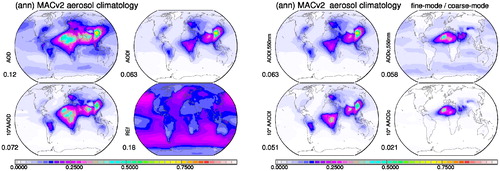
Figure 3 presents MACv2 annual average maps for the four properties of Fig. 1 (AOD, 10*AAOD, AODf and REf) and for AOD and 10*AAOD properties individually for fine-mode aerosol (AODf and 10* AAODf) and for coarse mode aerosol (AODc and 10*AAODc). While there is similarity in the maps for AOD and the order of magnitude lower AAOD for each size-mode, the spatial distributions between fine-mode (maxima over urban and biomass burning regions) and coarse mode (maxima of dust regions) are quite different. On a global average basis both size-modes contribute about evenly to the total AOD (ca. 50% vs. 50%), while the fine-mode contributes stronger to the AAOD (ca. 70% vs. 30%). The relative large AAODc contributions are the result of larger coarse-mode sizes over the Sahara region (as for a given refractive index imaginary part the mid-visible AAOD increases sharply with the coarse mode size). This AAODc size-dependence will be later used to extract size information on dust, whereas merged REf data constrain not only fine-mode aerosol sizes but also (fine-mode controlled) aerosol concentrations.

3. Components

3.1. Why components?

Tropospheric aerosol is always a mixture of many different sources. Breaking these spatially and in time varying mixtures down into radiatively well-defined components has several advantages. Most importantly, it allows a deterministic definition of aerosol radiative properties at other spectral regions (e.g. to satisfy satellite sensor or broadband radiative transfer requirements) and it allows to address radiative impacts of individual components (similar to approaches in ‘bottom-up’ modelling). Fortunately, MACv2 optical properties (AODf, AAODf, AODc and AAODc) and MACv2 fine-mode size information (REf) together provide sufficient detail so that not only an AOD separation into components is possible but also detail on component size and aerosol concentrations can be extracted.

3.2. What aerosol components are considered?

Adopting the aerosol component choices in global modelling (e.g. Kinne et al., 2006) five different components are considered with distinct differences in size and absorption. Components of sulfate (SU), organic carbon (OC), OC coated BC (OBC), mineral dust (DU) and sea-salt (SS) are selected and their size and composition properties are postulated. Assumed log-normal size-distributions and spectral refractive indices are presented in Table 1 and Figs. 4 and 5.

Fig. 4. Size-distributions of standard aerosol components (left block, with those for a water and ice cloud as reference) and for different sizes of sulfate and dust (right block, with effective radius values).

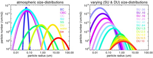
Fig. 5. Assumed real (left block) and imaginary part (right block) parts of the refractive indices for the different aerosol components (and for water and ice) of Fig. 4 for central wavelengths representing the 30 spectral bands of the RRTM radiative transfer model. References are Hale and Query (1973) for water, Warren (1984) for ice, Palmer and Williams (1975) for sulfate solutions, Nakayama et al. (2010) for organic aerosol, Bond (private communication) for BC, Nilsson (1979) for seasalt and Sokolik (private communication) for dust in the infrared and Wiedensohler (private communication) for dust in the solar region. Note, that the imaginary part of (only) 0.001 for dust was derived from by the mid-visible coarse-mode size and absorption of MACv2.

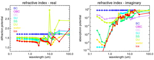
Table 1. Pre-defined aerosol types with assumed effective radii (RE), the associated log-normal size-distribution parameters (in bold) of mode radius (RM) and standard deviation (sd).

					at 550 nm wavelength
Aerosol type	Label	RE (μm)	RM (μm)	sd	RFR	RFI	SSA	opt.D	MEE m^2/g	N (#/m^2)
Soot (not used)	BC	.06	.03	1.7	1.70	.700	.155	0.004	8.9	3.4 e+ 12
Organic	OC	.12	.08	1.5	1.53	.005	.970	0.022	3.0	9.0 e+ 12
Soot + O.shell	OBC	.12	.08	1.5			.615	0.012		3.2 e+ 12
Sulfate^a	SU	.16	.08	1.7	1.43	.000	.999	0.037	3.2	1.9 e+ 13
Seasalt	SS	2.5	.75	2.0	1.50	.000	.999	0.028	0.31	2.6 e+ 10
Dust^b	DU	1.5	.93	1.55	1.53	.001	.962	0.031	0.27	3.4 e+ 10
Cloud water	Water	10	6.7	1.5	1.33	.000	.999	10.0		2.5 e+ 10
Cloud ice	Ice	40	20	1.7	1.31	.000	.999	0.5		1.1 e+ 08

^a Five extra sizes for SU: re = .06 μm (0.03 μm/1.7), .10 (.05/1.7), .26 (.13/1.7), .40 (.20/1.7), .64 (.32/1.7).

^b Four larger sizes for DU: re = 2.5 μm (1.2 μm/1.70), 4.0 (1.6, 1.85), 6.5 (2.0, 2.00), 10.0 (2.5, 2.50).

For the sulfate and dust components, extra size-distributions were pre-defined (as listed below the table). Also listed are the assumed mid-visible refractive indices real (RF_R) and imaginary (RF_I) parts. Global average mid-visible component aerosol optical depths of MACv2 (opt.D) illustrate the relative importance of components in terms of AOD and number concentrations (N). Also provided are associated estimates for the component mass extinction efficiency (MEE = AOD/mass). Finally, for comparisons also typical values of a cumulus water cloud (water) and a cirrostratus ice cloud (ice) are provided.

Hereby SU, OC and OBC types only contribute to the fine-mode AOD, whereas DU and SS types only contribute to the coarse-mode AOD. The OBC type (a BC soot core with an OC shell) accounts for the fine-mode solar absorption enhancement. The SU type represents the non-absorbing fine-mode type, including nitrate and fine-mode SS. SU and DU types are allowed to vary in size with effective radii ranging from 0.05 to 0.64 μm for SU and from 1.5 to 10 μm for DU.

3.3. How are components assigned?

To assign the pre-defined aerosol components to the MACv2 data (AODf, AODc, AAODf, AAODc), first the mid-visible AAOD for each component is determined via (MIE-) scattering simulations (Dave, 1968). With the size-distribution assumptions (as listed in of Table 1 and shown in Fig. 4), the three SU, OC and OBC components only contribute to the mid-visible AODf, while DU and SS component only contribute to the mid-visible AODc. Mid-visible absorption is indicated when the SSA falls significantly below 1.0. Thus, for the fine-mode only the OBC and OC components contribute to AAODf and only the DU component contributes to AAODc. To start the component assignment, some ancillary global monthly maps data are utilized:

• Local monthly (BC + OC)/(BC + OC + SU) fractions for AOD components from ‘bottom up’ global modelling provide initial guesses for AODf splits between absorbing (OBC, OC) and non-absorbing (SU) components.

• An ocean influence weight factors to avoid unrealistic sea-salt contributions over continents with a 1.0 weight over oceans but increasingly lower fractions with continental distances from the coast.

• Near-surface wind-speeds (in m/s) from re-analysis over oceans.

3.3.1. Coarse mode assignments

For the coarse mode component properties, ocean influence weight (ocean), near wind-speed (wind), local latitude (lat) and the sun’s seasonal varying latitude position (sun) define initial estimates for the coarse mode AOD of sea-salt (SS_AODc,ini) based on a fit to global monthly sea-salt mid-visible AOD maps from global ‘bottom-up’ modelling: $$\mathbf{SS}\_\mathbf{AODc},\mathbf{ini} = \mathbf{ocean} * 0.03*\mathbf{wind} *\left(2.0 - \text{cos}\left(2.0*\mathbf{lat} – \mathbf{lat,\; sun}/2.0\right)\right)$$

Any remaining coarse-mode AOD, after removing this seasalt AOD estimate, is attributed to dust. Now the (reasonable) assumption is made that the dust aerosol size increases with an increasing dust AOD. Hereby, an increasing dust size is expressed by an increasing absorption potential (1-SSA) starting from a value of 0.04 for the smallest considered mineral dust with an effective radius of 1.5 μm. Next, the MACv2 coarse-mode absorption (AAODc) is applied to assign the dust AOD (DU_AODc). Remember that only dust contributes to the mid-visible coarse-mode absorption, while sea-salt does not. $$\mathbf{DU}\_\mathbf{AODc} = \mathbf{AAODc}/\left(0.04+0.08*\mathbf{sqrt}\left(1- \mathbf{SS}\_\mathbf{AODc},\mathbf{ini}\right)\right), \mathbf{SS}\_\mathbf{AODc} = 1-\mathbf{DU}\_\mathbf{AODc}$$

An additional constraint is used that this DU_AODc estimate has to stay between a maximum (AODc –0.6*SS_AODc,ini) and a minimum (AODc –1.6*SS_AODs,ini) value, with respect to the initial seasalt AOD estimate. In rare cases of exceedance, absorption is allowed to be transferred between the size-modes, to assure that the overall aerosol absorption is maintained. Now with coarse-mode AOD (AODc) set, the coarse mode absorption potential (AAODc/DU_AODc) defines the effective radius for dust (DU), which is allowed to vary between 1.5 and 10 μm. Note that only with a relatively low refractive index imaginary part of only 0.001 for dust in the mid-visible region the AAODc data over the Sahara yield the expected mineral dust size increase near sources.

3.3.2. Fine mode assignments

For the fine-mode component properties, two carbon types are pre-defined. These are represented by a (in the mid-visible spectral region) weakly absorbing organic carbon (OC) type and a mixed carbon type (OBC) with a strongly absorbing soot (BC) core surrounded by a weakly absorbing OC shell. Both OC and OBC types were assigned an effective radius of 0.12 μm. Global modelling helps with an initial guess, how much of the fine-mode AODf of MACv2 is available for carbon. The fine-mode absorption AAODf of MACv2 then defines AODf contributions of OBC and OC types. Note, that the OBC contributes twice as much to the OC AOD than to the BC AOD. Then, the ratio between the assigned OC_AODf (from external and mixed contributions) and the BC_AODf is tested. If the OC_AODf/BC_AODf ratio remains below 5, then the model suggested OC/BC ratio carbon fraction is raised to 5 at the expense of the remaining (non-absorbing) fine-mode AOD, represented by the sulfate (SU) type. Finally, to reproduce the fine-mode effective radius (REf) of MACv2, the effective radius for SU is allowed to vary between 0.06 and 0.64 μm.

3.3.3. Component AOD maps

The resulting annual average mid-visible AOD attributions to the pre-defined components of Table 1 and Figs. 4 and 5 are presented in Fig. 6. The component AOD data for soot (BC – the BC in OBC), organic carbon (OC – the pure OC and the OC in OBC), total carbon (BC + OC) and non-absorbing fine mode (SU) are consistent with MACv2 properties for AODf and AAODf. And the component AOD attributions to mineral dust (DU) and seasalt (SS) are consistent with MACv2 properties for AODc and AAODc.

Fig. 6. Annual average AOD maps for today’s tropospheric aerosol for total (top left) and contributions by fine-mode aerosol sizes (top centre) and coarse-mode aerosol sizes (top right). In addition, consistent with mid-visible absorption data, component AOD values were assigned. The fine-mode AOD (‘aDU’ based on an anthropogenic dust fraction by P.Ginoux when applied to the MACv2 dust AOD, here multiplied by 10) is divided into contributions by BC (soot, here multiplied by 10), organic matter (OC) and sulfate (SU. where SU represents the non-absorbing fine-mode including nitrate and fine-mode sea-salt). The coarse mode AOD is split into contributions by seasalt and dust. In addition, annual AOD maps are presented for total carbon (OC + BC), for today’s anthropogenic dust (‘aDU’, here multiplied by 10, based on fractions provided by P. Ginoux) and two different estimates of today’s anthropogenic fine-mode AOD: ‘ant AC1’ is based on a fine-mode AOD fraction of AeroCom1 simulation and used in the MACv1, ‘ant AC2’ is based on a fine-mode AOD fraction of AeroCom2 and used in the MACv2. Values below the labels indicate global averages.

3.3.4. SU and DU size

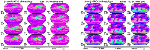
The size for the coarse-mode mineral dust component (DU) is defined by the strength of MACv2 AAODc for the MACv2 assigned DU_AODc (assuming a mid-visible refractive index imaginary part of 0.001). The size for the non-absorbing fine mode (SU) is defined by the assigned non-absorbing fine-mode SU_AOD and the MACv2 fine-mode radius (Ref) in the context of the OBC_AOD and OC_AOD 0.12 μm effective radii. Monthly maps for the resulting effective radii for DU and SU are presented in Fig. 7. Hereby, any particular size is approximated by a linear combination of the closest pre-defined sizes.

Fig. 7. Monthly effective radii (in μm) for dust (left block) based on MACv2 AAODc data and effective radii (in μm) for the non-absorbing fine-mode type (right block, SU), based on MACv2 REf data.

4. Anthropogenic

4.1. What is anthropogenic?

Anthropogenic contributions are essential for climate change assessments. Anthropogenic aerosol is defined by the extra aerosol since pre-industrial times as a result of human activities. While today’s aerosol properties can be measured, the needed pre-industrial reference requires many assumptions. Usually, there is a reliance on ‘bottom-up’ simulations with global models, where different back-scaling assumptions (e.g. considering changing population and burning habits) are applied to define emission scenarios at those pre-industrial times. MAC assumes that the additional anthropogenic emissions only contributed to the fine-mode aerosol properties. Thus, simulated AODf maps based on simulations of many different global models with today’s emissions and with pre-industrial emissions were compared. The increase in simulated AODf since pre-industrial times is quantified by the fraction of today’s AODf. This definition has the advantage that anthropogenic contributions are not influenced by variability to natural aerosol (e.g. wind-speed impacts on dust and humidity impacts on seasalt). Two different choices for anthropogenic fractions are offered. They yield quite different anthropogenic AOD maps when applied to the fine-mode AOD of MACv2.

4.2. Today’s anthropogenic AOD with AeroCom1

The first (and older) choice for today’s anthropogenic AOD is based on simulations with AeroCom 1 emissions (as they were prescribed in AeroCom phase1 experiments) for the years 2000 and 1750 (Dentener et al., 2006). This choice when applied to the fine-mode AOD of MACv2 yields the ‘ant AC1’- AOD distribution of Fig. 6. The associated global annual average mid-visible AOD is 0.040. This translates into ca 70% of today’s fine-mode AOD (AODf) and into ca 33% of today’s total AOD. This anthropogenic AOD was used in MACv1 (Kinne et al., 2013).

4.3. Today’s anthropogenic AOD with AeroCom2

The second (an newer) choice for today’s anthropogenic AOD is based on simulations with AeroCom 2 emissions (as they were prescribed in AeroCom phase2) experiments and suggested for the IPCC5 intercomparison for the years 2005 and 1850 (Lamarque et al., 2010). This choice, when applied to the fine-mode AOD of MACv2 yields the ‘ant AC2’- AOD distribution of Fig. 6. The associated global annual average mid-visible AOD is 0.031. This translates into ca 50% of today’s AODf and ca 25% of today’s total AOD. This anthropogenic AOD is the MACv2 default, which serves as basis in the plume approximation of MACv2-SP (Stevens et al., 2017).

4.4. Anthropogenic AOD as function of time

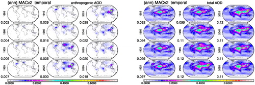
With the demand to address aerosol forcing as a function of time, year-to-year variations for anthropogenic AOD are considered. Following the temporal scaling approach of MACv1 (Kinne et al., 2013), the build-up of anthropogenic AOD since pre-industrial times (here the year 1850) is based on transient ‘bottom-up’ ECHAM simulation (Stier et al., 2006) with NIES emissions. Future anthropogenic AOD maps are defined by responses to regional changes in sulfate emissions based on the IPCC 5 RCP 8.5 future scenario. As increases to nitrate are ignored, future scenarios here are likely to have underestimated aerosol future impacts. Global distributions for mid-visible anthropogenic AOD and total AOD (note, only anthropogenic AOD was allowed to change) are presented in 20 year time-slices from 1865 to 2085 in Fig. 8. The maps show significant shifts for anthropogenic AOD (away from Europe and the US to SE Asia) in recent decades. The global average anthropogenic AOD today has reached its maximum with the expectation of an overall decline over the next decades (although strength of the decline is probably too strong as increasing nitrate contributions were ignored). The comparison to the total AOD development over time shows that anthropogenic AOD (but certainly not aerosol number) amounts only to a small fraction of the total AOD. Thus, in case natural variability is considered at least locally the anthropogenic AOD signal could get lost.

Fig. 8. Annual AOD (at 550 nm) maps in 20 steps from 1865 to 2085 for anthropogenic (left block) and total aerosol (right block) in the troposphere. Values below the label indicate global averages.

4.5. Anthropogenic SSA and anthropogenic ASY

Composition and size in radiative transfer are expressed via single scattering albedo (SSA) and asymmetry-factor (ASY), which are introduced in the next paragraph. In MACv2 these properties for anthropogenic aerosol are that of the fine-mode AOD and are not allowed to change over time. This is certainly a simplification, especially in the context of temporal change, as between 1950 and 1980 – with a stronger SU component – anthropogenic aerosol was less absorbing compared to anthropogenic composition of 100 years ago or today. Compared to AOD changes this simplification seems secondary.

5. Spectral extension

5.1. Why spectral extensions?

Radiative transfer applications require aerosol properties not just at a mid-visible wavelength. For instance, satellite remote sensing needs to apply aerosol properties at its sensor wavelengths and investigations of aerosol radiative effects (including climate impact investigations) require associated aerosol radiative properties at all solar and all infrared wavelengths of the applied radiative transfer code. The required aerosol radiative properties are the Aerosol Optical Depth (AOD, for aerosol amount), the Single Scattering Albedo (SSA, for the scattering potential) and the ASYmmetry-factor (ASY, to describe the scattering pattern). As a function of size (in comparison to the applied wavelength) and as a function of compositional mixture, all three aerosol radiative properties (AOD, SSA and ASY) vary with wavelength as a function of compositional mixture and size.

5.2. Components make it easy

Each pre-defined aerosol component is associated with spectrally varying refractive indices (e.g. as illustrated in Fig. 5 for the central wavelengths of the RRTM radiative transfer scheme). For each pre-defined aerosol component of Table 1 its spectral radiative properties (AOD, SSA and ASY) are easily defined via (MIE-) scattering methods. For spectral overall properties, these component properties just need to be combined according to AOD contributions by each component (as illustrated for annual averages of today’s aerosol in Fig. 6). Hereby, the mixing rules need to be remembered. While the combination of AOD is additive, combinations of SSA data require AOD weights and combinations of ASY data require AOD*SSA weights. Global annual averages of AOD, SSA and ASY for total, coarse-mode, fine-mode and anthropogenic aerosol are summarized in Table 2 at a few selected wavelengths. Associated annual maps are presented in the Appendix A.

Table 2. Global annual average aerosol radiative properties of today’s (tropospheric) aerosol.

		AOD				SSA			ASY
λ (μm)	Total	Coarse	Fine	Anthr^a	Total	Coarse	Fine	Total	Coarse	Fine
.45	.144	.058	.087	.043	.902	.905	.900	.718	.789	.670
.55	.122	.058	.063	.032	.941	.964	.919	.702	.767	.639
1.0	.081	.062	.019	.009	.956	.982	.870	.693	.736	.533
10	.049	.049			.580	.560		.605	.605

^a Anthropogenic SSA and ASY are that of the fine-mode.

Associated maps of regional distributions are presented in Appendix A.

Total (the sum of coarse and fine).

6. Vertical distribution

6.1. How vertically distributed?

All properties discussed so far refer to column averages. The aerosol vertical distribution is not only important for the IR radiative transfer (e.g. greenhouse effect of elevated mineral dust) but also for the solar radiative transfer – mainly via the relative altitude of aerosol to clouds. Clouds above aerosol cut off potential aerosol (solar) impacts, aerosol at cloud altitude may modify clouds and with clouds below aerosol any aerosol (solar) absorption is enhanced. The aerosol vertical distribution is prescribed separately for AODf and for AODc, as in MACv1. With the AOD scaling by size mode, the total values for SSA and ASY at each altitude will depend on the relative AOD contributions.

6.2. ECHAM modelling

The prescribed AOD vertical scaling in MACv2 is based on ‘bottom-up modelling. Multi-annual (1986–2006) monthly AOD scaling factors were created from ECHAM-HAM aerosol component simulation not just for total AOD but also more importantly separately for fine-mode and coarse mode AOD. The results of the ECHAM model were selected, because in comparisons to active remote sensing from space, ECHAM-HAM simulations demonstrated one of the better skill scores for AOD vertical distributions among the tested AeroCom models (Koffi et al., 2016). The global annual averages for AOD, AODf and AODc in a relative and an absolute sense are presented for four pre-defined tropospheric sub layers in Table 3. And the associated annual maps are presented in Appendix B.

Table 3. Annual averages of vertical distributions for the mid-visible AOD for four altitude (above sea-level) atmospheric layers (associated global maps are presented in Appendix B).

	Fraction of column AOD					AOD per layer
	CALv2 (z)	CALv3 (z)	ECHAM (z)			ECHAM(z) *MACv2
alt (km asl)	Total	Total	Total	Coarse	Fine	Total	Coarse	Fine
6–12	0.003	0.030	0.059	0.039	0.076	0.004	0.001	0.003
3–6	0.080	0.091	0.097	0.093	0.104	0.015	0.006	0.009
1–3	0.347	0.280	0.457	0.432	0.468	0.059	0.026	0.033
0–1	0.568	0.573	0.364	0.419	0.323	0.041	0.024	0.018

For total AOD, relative vertical distributions are compared between CALIPSO version 2 and 3 (columns 2 and 3) to ECHAM-HAM (column 4). The relative vertical distributions of ECHAM_HAM for coarse and fine-mode (columns 5 and 6) are applied the AODc and AODf of MACv2 to the layer AODs of columns 8 and 9.

6.3. CALIPSO data

Alternate data that could have been used to define aerosol vertical distributions are multi-annual (2006–16) mid-visible extinction profiles offered by CALIPSO lidar data from space. The most recent version 3 data (Tackett et al., 2018) as well as previous version 2 data (Winker et al., 2013; already tested for MACv1) place too much aerosol in a relative sense in the lowest atmospheric layers (0–1 km), as if some low clouds are mistaken for aerosol. This apparent altitude bias is illustrated in comparisons of relative altitude distributions for total AOD in Table 3 (averages) and Appendix B (maps). Another handicap for the use of CALIPSO data is that the needed separation into fine and coarse mode AOD contributions, which is needed for MAC climatology. The aerosol typing of CALIPSO is not precise enough for a quantitative extinction distinction into fine-mode and coarse mode contributions.

7. Cloud nuclei

7.1. Aerosol as cloud particle nuclei?

The cloud particle formation is usually helped, when aerosols are present and available. However, the affinity to serve as nuclei depends on aerosol composition, aerosol size and environment. Usually there is a distinction between nuclei for water clouds, referred to as Cloud Condensation Nuclei (CCN) and nuclei for ice clouds usually referred to as Ice Nuclei (IN). At lower altitude, where aerosol concentration is usually much higher, typical CCN concentrations range from about 30/cm3 in remote regions to more than 1000/cm³ in polluted regions. IN concentrations at a few/liter, in contrast, are much less frequent, with preferences for mineral dust and cold temperatures.

7.2. CCN concentrations

Usually all aerosols of the coarse-mode are large enough to serve as CCN, but only a fraction of the accumulation-mode aerosol qualifies. This fraction depends on the supersaturation (or upward wind at cloud-base altitude) and on the aerosol ability to attract water. The stronger the water attraction and/or the larger the supersaturations is, the smaller the aerosol sizes that can be activated. Four different supersaturations (0.05, 0.07, 0.10 and 0.20%) are assumed and the ability to attract water is expressed by the kappa parameter (Petters and Kreidenweis, 2007). Hereby component kappa values of BC (0.0) of OC (0.1) and non-absorbing fine-mode (SU, 0.8) are combined according to their MACv2 fine-mode mixture by mass (by applying the listed mass extinction efficiencies of Table 1, based on pre-defined density and size-distribution of a component). Then adding to the local kappa (k) value information on local temperature (T) and an applied supersaturation (SS) the critical dry radius cR_dry can be determined (Rose et al., 2008, formula A32): $$\mathbf{cR}\_\mathbf{dry} (\mathbf{um})=((4.0 *(0.66\mathbf{e}-6/\mathbf{T})**3)/(27*\mathbf{k}*\mathbf{ln}(\mathbf{SS}/100+1))**2.0)**.33$$

Next, the dry radius cR_dry needs to be converted into the wet radius cR_wet in order to be applicable to ambient fine-mode size distributions. This is done by a simple parametrization that depends on kappa k and the ambient relative humidity rh (Petters and Kreidenweis, 2007). As it is of interest to define the CCN concentrations near a low-altitude cloud base is assumed that the relative humidity (rh) is at 90%. $$\mathbf{cR}\_\mathbf{wet} \left(\mathbf{um}\right) = \mathbf{cR}\_\mathbf{dry} *\left(1 +\mathbf{k}*\mathbf{rh}/\left(1-\mathbf{rh}\right)\right)**.33, \text{rh}=0.9$$ cR_wet are applied to the log-normal size-distribution of the accumulation mode. This distribution is defined by the fine-mode AOD and the fine-mode effective radius of the MACv2 climatology and an assumed standard deviation of 1.7. All accumulation-mode particles larger than cR_wet and all coarse mode particles are counted as CCN. CCN concentrations at cloud base (ca. 1 km above ground) are determined by scaling column CCN data with the ratio of the fine-mode AOD fraction in the layer near the cloud-base and the layer thickness. CCN concentrations for different SS are presented in Fig. 9.

Fig. 9. Annual averages for critical radii (left block) at four different supersaturations: 0.05% (upper left), 0.07% (lower left), 0.1% (upper right) and 0.2% (lower right). Corresponding CCN concentrations at lower cloud base (at 1 km above the ground) at these supersaturations presented as well (right block). Hereby natural (left column), anthropogenic (mid column) and total contributions (right column) are compared.

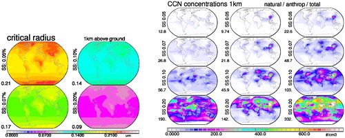
A supersaturation of 0.1% yields the most realistic MACv2 based CCN concentrations considering that at relative low CCN concentration almost all available CCN turn into Cloud Droplet Number Concentrations (CDNC). Also the comparison between natural and anthropogenic CCN concentrations is interesting as in regions of urban pollution anthropogenic concentrations can outumber natural concentrations by more than an order of magnitude.

7.3. In concentrations

It is assumed that only (coarse-mode) dust particles serve as IN and that this capability is sharply decreased when ambient temperatures get warmer than 238 K and even more so if warmer than 258 K. The T-reduced IN efficiency for dust concentrations is expressed by the T-factor.

Table

T-factor = exp(−A)*exp(−B)	A = 0 [T < 238 K]
	A = 0.5*T – 238, [238 K > T > 258 K]	B = 0 [T < 258 K]
	A = 10 [T > 258 K]	B = T – 258 [T > 258 K]

At three selected altitudes (7, 9 and 12 km), the dust component fractional AOD in that altitude layer (as defined by the coarse-mode vertical distribution) is divided by the layer thickness and then multiplied with the T-factor. The resulting ‘IN’ concentrations are presented in Fig. 10, where dust IN are missing over the tropics at 7 km altitude due to too warm temperatures and is also missing over high latitudes at 12 km altitude, at that altitude there is already well in the stratosphere.

Fig. 10. Annual average estimates for IN (dust) concentrations at 7 km (left), at 9 km (centre) and at 12 km (right). Note the log10 axis, so that 2 refers to 100 (/m³) and 6 to 1,000,000 (/m^–3).

8. Retrieval assistance

8.1. How to help satellite retrievals for aerosol?

The local and monthly variability captured by the aerosol properties of the MACv2 climatology can help under-determined satellite AOD retrievals with smart assumptions to aerosol size and absorption, although other uncertainties (e.g. the solar surface reflectance) remain open issues.

8.2. How to simplify size?

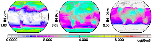
A bi-modal size-distribution is assumed, as in most aerosol retrievals models. Such a size-distribution shape is almost always retrieved by ground based sun-/sky photometry (Dubovik et al., 2002) showing a concentration minimum at radii near 0.5 μm. Thus, only two sizes are required. Based on frequency occurrences for effective radii of AERONET retrieved size-distribution samples, the most frequent effective radii are at 0.145 μm for the fine-mode and 1.9 μm for the coarse mode, as illustrated in Fig. 11. Corresponding selections for log-normal distribution parameters are 0.096 μm (fine) and 0.97 μm (coarse) for the mode radius (defining the size with the largest number concentration) and 1.5 (fine) and 1.7 (coarse) for standard deviation (defining the distribution width).

Fig. 11. Frequency of coarse-mode effective radius (x-axis) and fine-mode effective radius (y-axis) based on size-distribution detail of AERONET at all available sites (11,245 monthly averages in total).

8.3. How to simplify absorption?

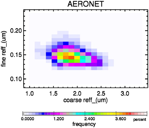
For both log-normal size distributions (to represent the fine-mode and the coarse mode) a non-absorbing (SSA = 1.0) composition and a maximum absorbing composition are defined. Hereby the maximum absorbing type for each size mode had to be at (or exceed the) largest absorption potential of the MACv2 climatology at each month and location: SSA = 0.77 for the fine-mode and SSA = 0.74 for the coarse mode. This way the local MACv2 absorption for each mode is simply determined by a mixture of two equal size aerosol types with different absorption potential. Annual averages of MACv2 suggested absorbing (and non-absorbing) type fractions are presented for fine-mode and coarse mode in Fig. 12.

Fig. 12. MACv2 associated mid-visible global maps for assistance in aerosol model choices in satellite retrievals. Annual averages (left block, left column) and seasonal averages (right block) are presented for total AOD at 550 nm and absorption type fractions for fine-mode AOD and coarse mode AOD. The AOD split is assigned by the fine mode fraction whose annual averages (left block, right column) are presented for twice the MACv2 AOD, for the standard MACv2 AOD and half the MACv2 AOD. In the context of the absorption fraction, absorption types have a single scattering albedo of .7693 (SSAf) and .7457 (SSAc) for fine-mode and coarse-mode, respectively, while the alternate scattering types have a single scattering albedo of 1.0. Note, the coarse mode absorption includes enhanced absorption by larger mineral dust sizes. Also shown in the left block are annual averages for (today’s) anthropogenic AOD and the complementary scattering fractions.

8.4. Steps of application

Once, look-up tables for the four aerosol types (2 sizes, 2 absorption strengths) have been created (to convert solar reflectance at any viewing direction into an AOD), contributing AOD values are combined into a total AOD, based on MACv2 local fractions for fine-mode AOD (AODf/AOD) and absorption type for each of the two size-modes. Then, the first guess for the total AOD is compared to the suggested total AOD of MACv2 at that location. In case of a difference, an alternate fine-mode AOD fraction (FMF) is applied for an improved final AOD estimate. The updated FMF is based on local multi-annual statistical relationships between AOD and FMF from the ICAP assimilation ensemble (Peng et al., 2019). The alternate AOD fine-mode fraction choice is based on multi-annual statistical relationships from ICAP satellite data assimilation ensemble between AOD and fine-mode AOD (Peng et al., 2019). Derived fine-mode fractions at twice and half the average AOD are compared to the fine mode fraction of the average AOD in Fig. 12.

9. Summary

9.1. Why MAC?

The Max-Planck Aerosol Climatology MAC informs on typical aerosol properties on a monthly global basis. The climatology offers likely aerosol properties which can be applied for more general evaluations of ‘bottom-up’ modelling and in satellite remote sensing. In its second version, MACv2 now extracts in a ‘top-down’ approach also compositional information, which in turn assists in a more consistent and confident spectral extension for the aerosol radiative properties needed in broadband radiative transfer simulations. The radiative properties, which can be accommodated to any radiative transfer scheme in global modelling, offer simple input for fast and more direct (since linked to observations of aerosol optics) alternative when estimating aerosol direct radiative impacts in global modelling. And with a simple satellite retrieval based relationship between aerosol and particle number concentrations (Kinne, 2019, Appendix A) also first order aerosol indirect radiative impacts can then be included.

9.2. How different is MACv2?

The MACv2 properties are listed in Table 4 and its annual global averages of selected aerosol properties compared to those of the older MACv1 version (Kinne et al., 2013), to the AeroCom 1 ensemble average (Kinne et al., 2006; Schulz et al., 2006) and to ICAP ensemble modelling (Peng et al., 2019).

Table 4. MACv2 properties in comparison to those of MACv1 (Kinne et al., 2013), of the AeroCom phase 1 median (Kinne et al., 2006) and of the ICAP ensemble modelling (Peng et al., 2019).

	MACv1	MACv2	AeroCom 1	ICAP
Spatial resolution (deg)	1 × 1	1 × 1	1 × 1	1 × 1
Temporal resolution	Monthly	Monthly	Monthly	3 hr
Reference year	2000	2005
Quality references	AERONET (->2010)	ANET + MAN (->2015)
Scaling background	AeroCom 1	Aerocom 1
AOD, 550 nm	0.13	0.12	0.12	0.14
Ant AOD, 550 nm	0.037 (Dentener emi.)	0.032 (Lamarque emi.)	0.029
AAOD, 550 nm	0.0054	0.0072	0.0043
FMF (AODf/AOD)	0.47	0.53	0.46	0.47
absFMF (AAODf/AAOD)	not available	0.71
Vertical distribution	ECHAM	ECHAM (CALIPSO)
Components	NO	YES
CCN (IN) estimates	NO	YES
Spectral rad. properties	AOD, SSA, ASY	AOD, SSA, ASY
TOA (all aerosol - sol + IR)	–1.6 W/m^2	–1.1 W/m^2
TOA (all aerosol - solar)	–2.1 W/m^2	–1.8 W/m^2
TOA (ant aerosol)	–0.5 W/m^2	–0.35 W/m^2	–0.22 W/m^2

The MACv2 radiative forcing estimates are from a companion paper (Kinne, 2019).

Compared to MACv1 (in terms of global annual averages), the anthropogenic fraction is lower, while the fine-mode AOD fraction is slightly higher. The (mid-visible) aerosol absorption is stronger, due to larger mineral dust sizes near sources regions, so that IR warming effects are increased in those regions.

In an application, the MACv2 associated aerosol radiative effects and the anthropogenic aerosol radiative forcing was determined (Kinne, 2019). The direct radiative forcing by today’s anthropogenic aerosol with MACv2 data is estimated at –0.35 W/m². This is lower than in MACv1, mainly due to a lower fine-mode anthropogenic fraction. In that paper also the definition of the anthropogenic fraction is identified to introduce the largest uncertainty. Even by only focusing on anthropogenic contributions to the fine-mode AOD in MACv2 (which removes potential variability by natural aerosol) questions remain about the accuracy of the assumed pre-industrial state. Even if regional emissions for present-day (PD) and pre-industrial conditions (PI) were accurate, there is still uncertainty from the processing of emissions in aerosol modules of global models. In addition, probable changes to anthropogenic fine-mode aerosol composition were ignored. For instance with stronger SU contributions a couple of decades ago both direct and indirect forcing efficiencies were probably more negative than today. The uncertain anthropogenic (or pre-industrial reference) definition is mainly driving the present day aerosol forcing uncertainties for the direct [–0.45 to –0.20 W/m², globally] and for the indirect (through clouds) effect [–1.2 to –0.4 W/m², globally] (Kinne, 2019).

9.3. What is next?

There are several elements for improvement. One limitation is that the climatology refers to an average year at current emissions. To improve the relevance to a particular year since 2000, fine-mode AOD and coarse-mode AOD regional anomalies (as offered via MODIS or MISR sensor data) could be applied. Another limitation is the current restriction to a single local aerosol property per-month. For future versions also local pdfs will be offered. This will allow to consider associations between different local aerosol properties such as a changing fine-mode fraction as function of AOD (as already offered by ICAP data). Also an update is needed for the temporal scaling for anthropogenic aerosol which currently goes back to MACv1. There are current efforts underway for an update based on ‘bottom-up’ transient AeroCom simulation, which also consider the nitrate component. These simulations will also inform on compositional changes of anthropogenic aerosol over time, which is considered as another element for improvement.

10. Resources

MACv2 properties are at ftp://ftp-projects.mpimet.mpg.de/aerocom/climatology/MACv2_2018/.

The data are placed in several subdirectories and a README file describes data content of file-names

• /550nm (mid-visible) aerosol properties at 550nm wavelength

• /CCN lower cloud-base condensation nuclei and critical radii at diff. supersaturation

• /detail ancillary data for radiative transfer simulations

• /documents some documentation and figures

• /forcing MACv2 associated radiative effects

• /programs fortran programs for the MAC v2 climatology

• /program_force fortran program for MAC associated radiative effects

• /retrieval MACv2 fields for under-determined solar reflection based AOD retrievals

• /spectral 2005 optical data at 3 different spectral resolutions: 20, 30 (RRTM), 31 bands

• /time same as in/spectral … but data for different years (from 1850 to 2100)

Acknowledgements

This study relied on observational data when possible. Central to the effort are data provided by the ground-based sunphotometer network of AERONET lead by B. Holben and the MAN network lead by A. Smirnov. Another essential element to this study is global model output from simulations with bottom-up processing in aerosol modules as part of the AeroCom initiative lead by M. Schulz and M. Chin. An ensemble median provides data on spatial context, estimates on aerosol anthropogenic fractions (also as a function of time) and aerosol vertical distribution. Thus, all modelling groups contributing to AeroCom experiments are acknowledged.

Disclosure statement

No potential conflict of interest was reported by the author.

Additional information

Funding

Finally, this work was support by EU-projects, in particular the FP7 EU-Bacchus project (603445) lead by U. Lohmann and by ESA’s climate initiative, in particular the aerosol-CCI effort lead by T. Popp and G. de Leeuw and coordinated by S. Pinnock.

Appendix A

Global maps for MACv2 annual maps of radiative properties (AOD, SSA and ASY) at selected wavelengths for today’s fine-mode, coarse-mode, total (coarse and fine) and anthropogenic aerosol are presented now

Fig. A1. MACv2 (2005) fine-mode radiative properties of AOD, SSA and ASY (at 0.45, 0.55, 1.0, 1.6 μm).

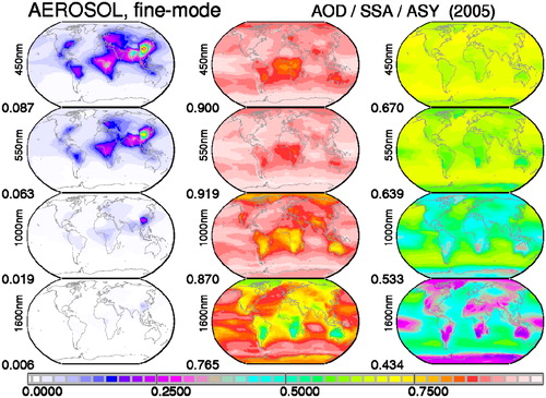
Fig. A2. MACv2 coarse-mode radiative properties of AOD, SSA and ASY (at 0.45, 0.55, 1.0, 10 μm).

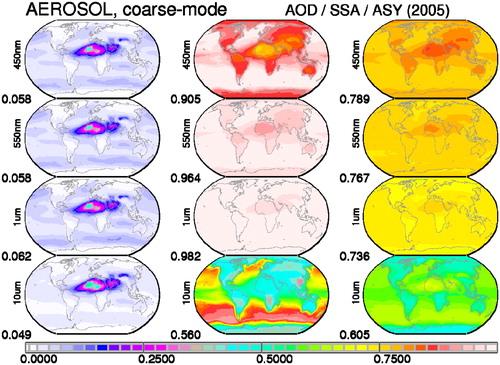
Fig. A3. MACv2 (2005) total aerosol properties of AOD, SSA and ASY (at 0.45, 0.55, 1.0, 10 μm).

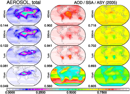
Fig. A4. MACv2 (2005) anthropogenic aerosol radiative properties of AOD, SSA and ASY (at .45, .55, 1.0, 1.6 μm) for today’s conditions. In MACv2 anthropogenic AOD is a fraction of the fine-mode AOD. Thus, anthropogenic SSA (composition) and ASY (size) properties are that of fine-mode aerosol. Local monthly anthropogenic SSA and ASY in MACv2 do not change for different years.

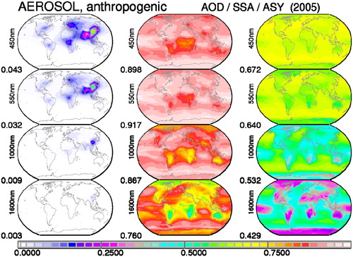
In all above plots, the values below the labels indicate global annual averages.

Appendix B

Global maps are presented for aerosol altitude distributions of AOD with respect 4 atmospheric layers: 0–1 km (row 4), 1–3 km (row 3), 3–6 km (row 2) and 6–12 km (row 1) above sea-level.

Fig. B1. ECHAM-HAM based multi-annual relative altitude distribution fractions (sum over all layer is 1) for total aerosol (left column), for the fine-mode (centre column) and for the coarse mode (right column).

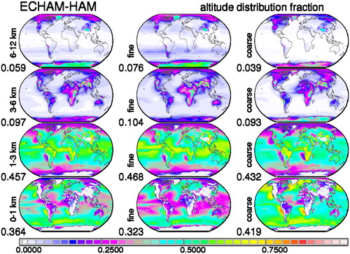
For MACv2, the relative vertical distribution for fine-mode and coarse mode of ECHAM-HAM are applied. The multiplication of these fractions with the AOD, AODf and AODc column values of MACv2 yields the vertical AOD distributions of Fig. B2.

The relative vertical distribution for total aerosol by ECHAM-HAM is mainly presented to illustrate in Fig. B3 the relative altitude AOD distribution differences of multi-annual CALIPSO data of version 2 and version 3 data. The CALIPSO data show in a relative sense much more aerosol in the lowest 1 km but it cannot be ruled out that this is an artefact (as low-level clouds may be counted as aerosol).

Fig. B2. MACv2 AOD vertical distribution with the ECHAM-HAM vertical scaling for total aerosol (left column), for fine-mode aerosol (centre column) and the coarse mode aerosol (right column).

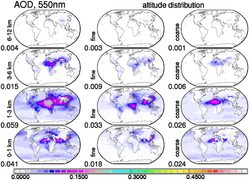
Fig. B3. Multi-annual relative altitude distribution fractions (sum over all layer is 1) for total aerosol between ECHAM_HAM (left column) and CALIPSO version 2 (centre column) and version 3 (right column).

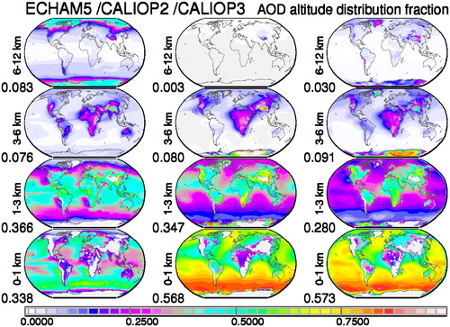
In all above plots, the values below the labels indicate global annual averages.

References

- Dave, J. V. 1968. Subroutines for Computing the Parameters of the Electromagnetic Radiation Scattered by Spheres. Report No. 320-3237, May; Palo Alto, Calif.: IBM Scientific Center.
- Dentener, F., Kinne, S., Bond, T., Boucher, O., Cofala, J. and co-authors. 2006. Emissions of primary aerosol and precursor gases in the years 2000 and 1750. Atmos. Chem. Phys. 6, 4321–4344. doi:10.5194/acp-6-4321-2006
- Dubovik, O., Holben, B., Eck, T. F., Smirnov, A., Kaufman, Y. J. and co-authors. 2002. Variability of absorption and optical properties of key aerosol types observed in worldwide locations. J. Atmos. Sci. 38, 580–608.
- Dubovik, O., Smirnov, A., Holben, B. N., King, M. D., Kaufman, Y. J. and co-authors . 2000. Accuracy assessments of aerosol optical properties retrieved from AERONET sun and sky-radiance measurements. J. Geophys. Res. 105, 9791–9806.
- Hale G. and Querry, M. 1973. Optical constants of water in the 200-nm to 200-microm wavelength region. Appl Opt. 12, 555–563. doi:10.1364/AO.12.000555
- Holben, B., Eck, T., Slutsker, I., Tanré, D., Buis, J. and co-authors. 1998. AERONET - A federated instrument network and data archive for aerosol characterization. Remote Sens Environ 66, 1–16. doi:10.1016/S0034-4257(98)00031-5
- Holben, B. N., Tanre, D., Smirnov, A., Eck, T. F., Slutsker, I. and co-authors. 2001. An emerging ground-based aerosol climatology: Aerosol Optical Depth from AERONET. J. Geophys. Res. 106, 12067–12097.
- Kinne, S. 2019. Aerosol radiative effects with MACv2. Atmos. Chem. Phys. Discuss.
- Kinne, S., Lohmann, U., Feichter, J., Schulz, M., Timmreck, C. and co-authors. 2003. Monthly averages of aerosol properties: A global comparison among models, satellite data, and AERONET ground data. J. Geophys. Res. 108, 4634.
- Kinne, S., O'Donnel, D., Stier, P., Kloster, S., Zhang, K. and co-authors. 2013. MAC-v1: A new global aerosol climatology for climate studies. J. Adv. Model. Earth Syst. 5, 704–740. doi:10.1002/jame.20035
- Kinne, S., Schulz, M., Textor, C., Guibert, S., Bauer, S. and co-authors. 2006. An AeroCom initial assessment – optical properties in aerosol component modules of global models. Atmos. Chem. Phys. 6, 1–22.
- Koffi, B. M., Schulz, F. M., Bréon, F., Dentener, B. M., Steensen, J. and co-authors. 2016. Evaluation of the aerosol vertical distribution in global aerosol models through comparison against CALIOP measurements: AeroCom phase II results. J. Geophys. Res. Atmos. 121, 7254–7283. doi:10.1002/2015JD024639
- Köpke, P., Heß, M., Schuldt, I. and Shettle, E. 1997. Global aerosol dataset. Report No. 243, Max-Planck Institut für Meteorologie, Hamburg, Germany.
- Lamarque, J.-F., Bond, T. C., Eyring, V., Granier, C., Heil, A. and co-authors. 2010. Historical (1850-2000) gridded anthropogenic and biomass burning emissions of reactive gases and aerosols: methodology and application. Atmos. Chem. Phys. 10, 7017–7039. doi:10.5194/acp-10-7017-2010
- Nakayama, T., Matsumi, Y., Sato, K., Imamura, T., Yamazaki, A., and Uchiyama, A. 2010. Laboratory studies on optical properties of secondary organic aerosols generated during the photooxidation of toluene and the ozonolysis of α-pinene. J. Geophys. Res. 115, D24204. doi:10.1029/2010jd014387
- Nilsson, B. 1979. Meteorological influence on aerosol extinction in the 0.2–40-μm wavelength range. Applied Optics 18, 3457–3473. doi:10.1364/AO.18.003457
- O’Neill, N., Eck, T. F., Smirnov, A., Holben, B. N. and Thulasiraman, S. 2003. Spectral discrimination of coarse and fine mode optical depth. J. Geophys. Res. 108, 4559–4573.
- Palmer, K. and Williams, D. 1975. Optical constants of sulfuric acid; application to the clouds of venus? Applied Optics 14, 208–219. doi:10.1364/AO.14.000208
- Peng, Y., Reid, J. S., Hyer, E. J., Sampson, C. R., Rubin, J. I. and co-authors. 2019. Current state of the global operational aerosol multi-model ensemble: an update from the International Cooperative for Aerosol Prediction (ICAP). Q. J. R. Meteorol. Soc. doi:10.1002/qj.3497
- Petters, M. D. and Kreidenweis, S. 2007. A single parameter representation of hygroscopic growth and cloud condensation nucleus activity. Atmos. Chem. Phys. 7, 1961–1971. doi:10.5194/acp-7-1961-2007
- Rose, D., Gunthe, S., Mikhailov, E., Frank, G., Dusek, U. and co-authors. 2008. Calibration and measurement uncertainties of a continuous-flow cloud condensation nuclei counter (DMT–CCNC): CCN activation of ammonium sulfate and sodium chloride aerosol particles in theory and experiment. Atmos. Chem. Phys. 8, 1153–1179. doi:10.5194/acp-8-1153-2008
- Schulz, M., Textor, C., Kinne, S., Balkanski, Y., Bauer, S. and co-authors. 2006. Radiative forcing by aerosols as derived from the AeroCompresent-day and pre-industrial simulations. Atmos. Chem. Phys. 6, 5225–5246. doi:10.5194/acp-6-5225-2006
- Smirnov, A., Holben, B., Giles, D., Slutsker, I., O'Neill, N. and co-authors. 2011. Maritime aerosol network as a component of AERONET – first results and comparison with global aerosol models and satellite retrievals. Atmos. Meas. Tech. 4, 583–597. doi:10.5194/amt-4-583-2011
- Smirnov, A., Holben, B. N., Slutsker, I., Giles, D. M., McClain, C. R. and co-authors. 2009. Maritime Aerosol Network as a component of Aerosol Robotic Network. J. Geophys. Res. 114, D06204.
- Stevens, B., Fiedler, S., Kinne, S., Peters, K., Rast, S. and co-authors. 2017. MACv2-SP: a parameterization of anthropogenic aerosol optical properties and an associated Twomey effect for use in CMIP6. Geosci. Model Dev. 10, 433–452. doi:10.5194/gmd-10-433-2017
- Stier, P., Feichter, J., Roeckner, E., Kloster, S. and Esch, M. 2006. The evolution of the global aerosol system in a transient climate simulation from 1860 to 2100. Atmos. Chem. Phys. 6, 3059–3076. doi:10.5194/acp-6-3059-2006
- Tackett, J. L., Winker, D. M., Getzewich, B. J., Vaughan, M. A., Young, S. A. and co-authors. 2018. CALIPSO lidar level 3 aerosol profile product. Atmos. Meas. Tech. 11, 4129–4152. 2018 doi:10.5194/amt-11-4129-2018
- Textor, C., Schulz, M., Guibert, S., Kinne, S., Balkanski, Y. and co-authors. 2007. The effect of harmonized emissions on aerosol properties in global models – an Aerocom experiment. Atmos. Chem. Phys. 7, 4489–4501. doi:10.5194/acp-7-4489-2007
- Warren, S. 1984. Ultraviolet to the microwave. Applied Optics. 23, 1206–1225. doi:10.1364/AO.23.001206
- Winker, D., Tackett, J., Getzewich, B., Liu, Z., Vaughan, M. and co-authors. 2013. The global 3-D distribution of tropospheric aerosols as characterized by CALIOP. Atmos. Chem. Phys. 13, 3345–3361. doi:10.5194/acp-13-3345-2013