Picture Fuzzy N-Soft Sets and Their Applications in Decision-Making Problems

Abstract

In this article, firstly, we describe picture fuzzy N-soft sets (PFN-SSs) as a generalization of picture fuzzy sets (PFSs) and N-soft sets (N-SS) by observing that one of the essential concept of neutral grade is missing in intuitionistic fuzzy N-SS (IFN-SS) theory. The concept of neutrality grade can be observed in the situation when we encounter human views including more answers of type: yes, abstain, no, refusal. For instance, in election the election commission or election council issues voting papers for the candidate. The voting outcomes are categorized into 4 groups with the number of papers namely, vote for, abstain, vote against, and refusal voting. Further, We define the fundamental properties of PFN-SS and introduce M-subset, F-subset, compliment, intersections, unions, of PFN-SS and give their examples. Secondly, we define an algorithm to cope with PFN-SS data which is more generalized then the algorithm defined for IFN-SS. To show the advantage and usefulness of the defined technique, we give two examples from real life by utilizing PFN-SS data. The result shows in the comparison that our initiated method is more general and suitable than the IFN-SS, fuzzy N-SS (FN-SS), and N-SS.

KEYWORDS:

• Picture fuzzy N-soft sets
• intuitionistic fuzzy N-soft sets
• N-soft sets
• soft sets
• picture fuzzy soft sets
• decision-making

1. Introduction

The majority of the real-life problems include uncertainty and vagueness in data. Handling such data is a big issue in many fields like engineering, social sciences, medical sciences, and economics. In light of this worry, Zadeh [1] presented fuzzy sets (FSs). The idea of FS is truly manageable because it catches vague and uncertain data. In FSs theory the grade of membership belongs to a closed interval [0,1]. Nonetheless, it may not generally be right to assume that the grade of non-membership in FS is equivalent to 1 minus the grade of membership, due to the presence of the degree of uncertainty or indeterminacy. Consequently, Atanassov [2] defined the idea of intuitionistic FSs (IFSs), which is a suitable generalisation of FSs. After this, Cuong [3] characterised a new idea by putting an additional grade which is a grade of neutral membership, and named it to picture FS (PFS). It triply contains positive membership, neutral membership, and negative membership. Researchers show interest to work on PFS because it is straightforwardly applied to tackle everyday life issues. Some fuzzy logic operators for PFSs were given by Cuong and Van Hai [4]. Luo and Zhang et al. [5] described new similarity measures for PFSs and its applications. Khan et al. [6] presented bi-parametric distance and similarity measures of PFSs and their applications in medical diagnosis. Khan et al. [7] presented distance and similarity measures for spherical FSs and their application in selecting mega projects. Mahmood et al. [8] gave the concept of complex hesitant FSs (CHFSs). The idea of complex dual hesitant FSs (CDHFSs) was given by Mahmood et al. [9].

Nonetheless, Molodtsov [10] showed that few challenges of the previously mentioned notions can be overwhelmed with the establishment of parameterised interpretation of the universe, an idea giving rise to soft sets (SSs) [10]. Soon, Maji et al. [11] established few algebraic operations in SS theory, which currently assume a significant part in fields such as DM [12–16] and data analysis [17]. Ali et al. [18] defined some modified operations in SS theory. Anyway, the information frequently comes across in a complex structure. A lot of researchers have developed new models to overcome such types of data and merge the advantages of the presented models. These models are developed to resolve a vast range of DM issues since they have more advantages than the original models. For example, by the mixture of FSs and SSs, Maji et al. [19] defined a new model, called fuzzy SS (FSS). A new idea of DM issues based on FSSs was given by Alcantud [20]. Maji et a. [21] gave the idea of intuitionistic FSSs (IFSSs) which is a mixture of IFSs and SSs. Khan et al. [22] defined a novel approach to generalised IFSSs and its application in decision support system. Khan et al. [23] gave another view on generalised interval-valued IFSSs. The renewable energy source selection by remoteness index-based VIKOR method for generalised IFSSs was presented by khan et al. [24]. The distance and similarity measures of generalised IFSSs were defined by khan and Kumam [25]. Yang et al. [26] defined an adjustable soft discernibility matrix based on PFSSs and its application in DM. Khan et al. [27] defined generalised PFSSs and described some modified operations for PFSSs. Jan et al. [28] defined multi-valued PFSSs and their applications in group DM problems. The applications of generalised PFSSs in concept selection were given by khan et al. [29]. Khan et al. [30] described an adjustable weighted soft discernibility matrix based on generalised PFSS and its applications in decision-making. Khan et al. [31] defined a theoretical-justifications for the empirically successful VIKOR approach to multi-criteria DM. Akram et al. [32] described hybrid DM frameworks under complex spherical FSSs.

We noted a lot of modifications of SSs in various directions such as probabilistic SS theory [33], bijective SSs [34], and fuzzy bipolar SSs [35]. Specifically, Fatimah et al. [36] introduced N-SS as a modification of SS that takes into consideration multinary parameterised interpretation of the universe. Alcantud et al. [37] interpreted an N-SS approach to rough sets. Kamaci and Petchimuthu [38] defined bipolar N-SS theory with applications. Fatimah and Alcantud [39] presented the multi-fuzzy N-SS and its applications to DM. Akram et al. [40] defined complex neutrosophic N-SS. A hybrid DM approach under complex Pythagorean fuzzy N-SS was given by Akram et al. [41]. Mahmood et al. [42] defined the complex picture fuzzy N-SSs. Akram et al. [43] provided the parameter reductions in N-SSs and their applications in DM. The inspiration for their defined N-SS is given as. An investigation of models with SSs as one of their components had indicated that the authors were motivated by SSs and their work of assessments (memberships are either 0 or 1) or the situation with partial memberships containing in [0,1] [17,44]. Anyway, a lot of real-life DM issues contain information with discrete and non-binary structure, which consequently didn’t in the shape of those formats. It is simple to create examples including non-binary assessments. We frequently get them in ranking or rating position such as websites comparing software, movies, or mobile phones. Even though they frequently appear as several stars or dots (such as four stars, three stars, two stars, one star), which can simply be linked with natural numbers. As additional evidence of the capability of N-SS theory, Akram et al. [45] merge the N-SS with FS to defined FN-SS. After this, Akram et al. [46] defined the notion of IFN-SS which the mixture of IFS and N-SS.

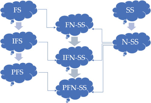
IFN-SS is a good tool to deal with uncertainty and is in the form of $(\mathrm{K},((\mathrm{I},\mathfrak{T},N)\left)\right)$, where $\mathrm{K}$ is an intuitionistic fuzzy number and $(\mathrm{I},\mathfrak{T},N)$ is N-SS. It is noticed that one of the essential notion of neutrality grade is missing in IFN-SS theory. The notion of neutrality grade can be observed in the situation when we encounter human views including more answers of kinds: yes, abstain, no, and refusal. For instance, in an election, the election commission or election council issues ballot papers for the contestant. The voting outcomes are categorised into 4 groups with the number of papers, i.e. vote for, abstain, vote against, and refusal voting. Class of abstain signifies that the voting paper is a white paper refusing both agree and disagree for the contestant but still takes the vote. Class of refusal voting is either unacceptable papers or avoiding the vote. Nevertheless, the neutral grade can be taken into the consideration in medical diagnosis. For example, there may not influence the symptoms of fever, leg pain on the diseases heart problem, and brain tumour. Likewise, the symptoms of heart problems and blood cancer have a neutral influence on the diseases flu, corona, TB, etc. In IFN-SS we lost some of the important information in the shape of neutral grade which effect the end result in the decision-making problem. To overcome this and other weaknesses presented in some existing models in this article, we presented the notion of PFN-SS which is the extension of IFN-SS, FN-SS and will perform better than IFN-SS in DM. The geometrical representation of the PFN-SS is given in Figure 1.

Figure 1. Flowchart of FSs, SSs, and their generalisation.

The organisation of this article as follows:

• Section 2 is consists with preliminaries in which we recall few basic definitions such as FSs, IFS, PFSs, SSs, FSS, IFSS, PFSS N-SSs, and IFN-SS. We also recall the basic properties of some of the above basic definitions.

• Section 3 is a picture fuzzy N-Soft set in which we initiate PFN-SSs which is a mixture of PFSs and N-SS and explain it by giving examples. We also initiate the fundamental properties of PFN-SS in Section 3.

• Section 4 of this article is applications of PFN-SS in which we introduce an algorithm to cope with PFN-SS data and to show the advantage and usefulness of the defined technique.

• Section 5 is a comparison in which we do a comparison of our initiated model with IFN-SS.

• In Section 6, the conclusion and future study of the proposed work are presented.

2. Preliminaries

In this section, let us recall few basic definitions such as FSs, IFS, PFSs, SSs, FSS, IFSS, PFSS N-SSs, and IFN-SS. We also recall the basic properties of some of the above basic definitions. $\mathfrak{U}\ne set$ be set of universe and $\mathrm{A}$ be set of attributes throughout this manuscript.

Zadeh [1], defined the idea of FS, which gives a powerful structure to dealing with uncertainty.

Definition 1:

[1] A FS $\mathfrak{D}$ over $\mathfrak{U}$ is given as

$\mathfrak{D}=\left\{\left(\mathfrak{u},{\xi }_{\mathfrak{D}}\left(\mathfrak{u}\right)\right):\mathfrak{u}\in \mathfrak{U}\right\}$,

where ${\xi }_{\mathfrak{D}}:\mathfrak{U}\to \left[0,1\right]$ is a grade of membership. For every $\mathfrak{u}\in \mathfrak{U}$, ${\xi }_{\mathfrak{D}}\left(\mathfrak{u}\right)$ describes the degree to which $\mathfrak{u}$ be a member of FS $\mathfrak{D}$. The pair $\left(\mathfrak{u},{\xi }_{\mathfrak{D}}\left(\mathfrak{u}\right)\right)$ is called fuzzy number (FN)

In [1] Zadeh described some basic operations which are as follows:

Definition 2:

[1]Let $\mathfrak{D}=\left(\mathfrak{u},{\xi }_{\mathfrak{D}}\left(\mathfrak{u}\right)\right)$ and $\mathcal{E}=\left(\mathfrak{u},{\xi }_{\mathcal{E}}\left(\mathfrak{u}\right)\right)$ be two FNs. Then

1. $\mathfrak{D}=\mathcal{E}\iff {\xi }_{\mathfrak{D}}\left(\mathfrak{u}\right)={\xi }_{\mathcal{E}}\left(\mathfrak{u}\right)$;

2. $\mathfrak{D}\subseteq \mathcal{E}\iff {\xi }_{\mathfrak{D}}\left(\mathfrak{u}\right)\le {\xi }_{\mathcal{E}}\left(\mathfrak{u}\right);$

3. ${\mathfrak{D}}^c=\left(\mathfrak{u},1-{\xi }_{\mathfrak{D}}\left(\mathfrak{u}\right)\right)$;

4. $\mathfrak{D}\cup \mathcal{E}=\left(\mathfrak{u},max\left({\xi }_{\mathfrak{D}}\left(\mathfrak{u}\right),{\xi }_{\mathcal{E}}\left(\mathfrak{u}\right)\right)\right)$;

5. $\mathfrak{D}\cap \mathcal{E}=\left(\mathfrak{u},min\left({\xi }_{\mathfrak{D}}\left(\mathfrak{u}\right),{\xi }_{\mathcal{E}}\left(\mathfrak{u}\right)\right)\right)$.

In [2], Atanassov defined the concept of IFS

Definition 3:

[2] An IFS over $\mathfrak{U}$ is given as $\mathfrak{D}=\left\{\left(\mathfrak{u},\left({\xi }_{\mathfrak{D}}\left(\mathfrak{u}\right),{\vartheta }_{\mathfrak{D}}\left(\mathfrak{u}\right)\right)\right):\mathfrak{u}\in \mathfrak{U}\right\},$ where ${\xi }_{\mathfrak{D}}:\mathfrak{U}\to \left[0,1\right]$ is a grade of membership and ${\vartheta }_{\mathfrak{D}}:\mathfrak{U}\to \left[0,1\right]$ is the grade of non-membership with a condition that $0\le {\xi }_{\mathfrak{D}}\left(\mathfrak{u}\right)+{\vartheta }_{\mathfrak{D}}\left(\mathfrak{u}\right)\le 1$ for each $\mathfrak{u}\in \mathfrak{U}$. The pair $\left(\mathfrak{u},\left({\xi }_{\mathfrak{D}}\left(\mathfrak{u}\right),{\vartheta }_{\mathfrak{D}}\left(\mathfrak{u}\right)\right)\right)$ is called intuitionistic FN (IFN).

In [3], Cuong described PFSs by putting an additional grade of membership called the grade of neutral membership. Mainly, the notion of PFS may be appropriate in the environment when one faces human judgments containing more replies of the form: yes, no, abstain refusal. Voting is the best example of PFS.

Definition 4:

[3] A PFS over $\mathfrak{U}$ is given as $\mathfrak{D}=\left\{\left(\mathfrak{u},\left({\xi }_{\mathfrak{D}}\left(\mathfrak{u}\right),{\delta }_{\mathfrak{D}}\left(\mathfrak{u}\right),{\vartheta }_{\mathfrak{D}}\left(\mathfrak{u}\right)\right)\right):\mathfrak{u}\in \mathfrak{U}\right\},$ where ${\xi }_{\mathfrak{D}}:\mathfrak{U}\to \left[0,1\right]$, is a grade of membership, ${\delta }_{\mathfrak{D}}:\mathfrak{U}\to \left[0,1\right]$ is the grade of neutral membership and ${\vartheta }_{\mathfrak{D}}:\mathfrak{U}\to \left[0,1\right]$ is the grade of non-membership with a condition that $0\le {\xi }_{\mathfrak{D}}\left(\mathfrak{u}\right)+{\delta }_{\mathfrak{D}}\left(\mathfrak{u}\right)+{\vartheta }_{\mathfrak{D}}\left(\mathfrak{u}\right)\le 1$ for each $\mathfrak{u}\in \mathfrak{U}$. The pair $\left(\mathfrak{u},\left({\xi }_{\mathfrak{D}}\left(\mathfrak{u}\right),{\delta }_{\mathfrak{D}}\left(\mathfrak{u}\right),{\vartheta }_{\mathfrak{D}}\left(\mathfrak{u}\right)\right)\right)$ is called picture FN (PFN).

In [3] Cuong also defined basic operations of PFS which are given below

Definition 5:

[3]

Let $\mathfrak{D}=\left(\mathfrak{u},\left({\xi }_{\mathfrak{D}}\left(\mathfrak{u}\right),{\delta }_{\mathfrak{D}}\left(\mathfrak{u}\right),{\vartheta }_{\mathfrak{D}}\left(\mathfrak{u}\right)\right)\right)$ and $\mathcal{E}=\left(\mathfrak{u},\left({\xi }_{\mathcal{E}}\left(\mathfrak{u}\right),{\delta }_{\mathcal{E}}\left(\mathfrak{u}\right),{\vartheta }_{\mathcal{E}}\left(\mathfrak{u}\right)\right)\right)$ be two PFNs. Then

1. $\mathfrak{D}=\mathcal{E}\iff {\xi }_{\mathfrak{D}}\left(\mathfrak{u}\right)={\xi }_{\mathcal{E}}\left(\mathfrak{u}\right),{\delta }_{\mathfrak{D}}\left(\mathfrak{u}\right)={\delta }_{\mathcal{E}}\left(\mathfrak{u}\right),{\vartheta }_{\mathfrak{D}}\left(\mathfrak{u}\right)={\vartheta }_{\mathcal{E}}\left(\mathfrak{u}\right)$;

2. $\mathfrak{D}\subseteq \mathcal{E}\iff {\xi }_{\mathfrak{D}}\left(\mathfrak{u}\right)\le {\xi }_{\mathcal{E}}\left(\mathfrak{u}\right),{\delta }_{\mathfrak{D}}\left(\mathfrak{u}\right)\le {\delta }_{\mathcal{E}}\left(\mathfrak{u}\right)$, ${\vartheta }_{\mathfrak{D}}\left(\mathfrak{u}\right)\ge {\vartheta }_{\mathcal{E}}\left(\mathfrak{u}\right)$;

3. ${\mathfrak{D}}^c=\left(\mathfrak{u},{\vartheta }_{\mathfrak{D}}\left(\mathfrak{u}\right),{\delta }_{\mathfrak{D}}\left(\mathfrak{u}\right),{\xi }_{\mathfrak{D}}\left(\mathfrak{u}\right)\right)$;

4. $\mathfrak{D}\cup \mathcal{E}=\left(\mathfrak{u},max\left({\xi }_{\mathfrak{D}}\left(\mathfrak{u}\right),{\xi }_{\mathcal{E}}\left(\mathfrak{u}\right)\right),min\left({\delta }_{\mathfrak{D}}\left(\mathfrak{u}\right),{\delta }_{\mathcal{E}}\left(\mathfrak{u}\right)\right),min\left({\vartheta }_{\mathfrak{D}}\left(\mathfrak{u}\right),{\vartheta }_{\mathcal{E}}\left(\mathfrak{u}\right)\right)\right)$;

5. $\mathfrak{D}\cap \mathcal{E}=\left(\mathfrak{u},min\left({\xi }_{\mathfrak{D}}\left(\mathfrak{u}\right),{\xi }_{\mathcal{E}}\left(\mathfrak{u}\right)\right),min\left({\delta }_{\mathfrak{D}}\left(\mathfrak{u}\right),{\delta }_{\mathcal{E}}\left(\mathfrak{u}\right)\right),max\left({\vartheta }_{\mathfrak{D}}\left(\mathfrak{u}\right),{\vartheta }_{\mathcal{E}}\left(\mathfrak{u}\right)\right)\right)$.

In [10], Molodtsov described the SS which is entirely a new tool to cope with the uncertainties from a parametrisation opinion. Most of the time the parameter set contains characteristics, attributes, or properties of the alternatives.

Definition 6:

[10] A pair $\left(\mathrm{I},\mathfrak{T}\right)$ is a SS over $\mathfrak{U}$ where $\mathrm{I}:\mathfrak{T}\to P\left(\mathfrak{U}\right)$ be set-valued function and $\mathfrak{T}\subseteq \mathrm{A}$.

Maji et al. [19] described the FSS, which is a mixture of FS and SS. In FSS, each parameter should be represented by grade of membership, as in real-world, the opinion of the people is represented by some degree of imprecision.

Definition 7:

[19] A pair $({\mathrm{I}}^{\mathrm{\prime }},\mathfrak{T})$ represents an FSS over $\mathfrak{U}$ if ${\mathrm{I}}^{\mathrm{\prime }}:\mathfrak{T}\to \mathfrak{F}\mathcal{S}\left(\mathfrak{U}\right),\mathfrak{T}\subseteq \mathrm{A}$, where $\mathfrak{F}\mathcal{S}\left(\mathfrak{U}\right)$ represents the set of all FS of $\mathfrak{U}$.

Maji et al. [21] described the IFSS, which is a mixture of IFS and SS.

Definition 8:

[21] A pair $({\mathrm{I}}^{\mathrm{\prime }\mathrm{\prime }},\mathfrak{T})$ describes an IFSS over $\mathfrak{U}$ if ${\mathrm{I}}^{\mathrm{\prime }\mathrm{\prime }}:\mathfrak{T}\to I\mathfrak{F}\mathcal{S}\left(\mathfrak{U}\right),\mathfrak{T}\subseteq \mathrm{A}$, where $I\mathfrak{F}\mathcal{S}\left(\mathfrak{U}\right)$ represents the set of all IFS of $\mathfrak{U}$.

In [26], Yang described the PFSS, a mixture of PFS and SS. In PFSS, we can view vagueness from a parametrisation opinion in a picture fuzzy (PF) environment.

Definition 9:

[26] Let $\mathcal{P}\mathfrak{F}\mathcal{S}\left(\mathfrak{U}\right)$ be a set of all PFSs over $\mathfrak{U}$. A pair $({\mathrm{I}}^{\mathrm{\prime }\mathrm{\prime }\mathrm{\prime }},\mathfrak{T})$ is called the PFSS over $\mathfrak{U}$, where ${\mathrm{I}}^{\mathrm{\prime }\mathrm{\prime }\mathrm{\prime }}:\mathfrak{T}\to \mathcal{P}\mathfrak{F}\mathcal{S}\left(\mathfrak{U}\right),\mathfrak{T}\subseteq \mathrm{A}$.

Fatimah et al. [36] described the idea of N-SS which is the modification of SS.

Definition 10:

[36] Let a universal set of alternatives be $\mathfrak{U}$ and $\mathrm{A}$ be attributes. A triplet $\left(\mathrm{I},\mathfrak{T},N\right)$ is called N-SS over $\mathfrak{U}$, where $\mathrm{I}:\mathfrak{T}\to 2^{\mathfrak{U}\times \mathcal{Y}}=P\left(\mathfrak{U}\times \mathcal{Y}\right),\mathfrak{T}\subseteq \mathrm{A}$, with the property that for every $\mathcal{t}\in \mathfrak{T}$ and $\mathrm{\exists }$ a unique $\left(\right(\mathfrak{u},{\mathcal{y}}_{\mathcal{t}})\in P(\mathfrak{U}\times \mathcal{Y}\left)\right)$ such that $(\mathfrak{u},{\mathcal{y}}_{\mathcal{t}})\in \mathrm{I}\left(\mathcal{t}\right)$, $\mathfrak{u}\in \mathfrak{U},{\mathcal{y}}_{\mathcal{t}}\in \mathcal{Y}=\{0,1,2,\dots ,N-1\}$ be ordered grades set.

Fatimah et al. [36] also described the extended and restricted intersection and union of N-SS which is given below

Definition 11:

[36] Let ${\mathrm{\Theta }}_1=\left({\mathrm{I}}_1,{\mathfrak{T}}_1,N_1\right)$ and ${\mathrm{\Theta }}_2=\left({\mathrm{I}}_2,{\mathfrak{T}}_2,N_2\right)$ be two N-SSs with ${\mathfrak{T}}_1\cap {\mathfrak{T}}_2\ne set$. Then the restricted union and the intersection of ${\mathrm{\Theta }}_1$ and ${\mathrm{\Theta }}_2$ are described below: ${\mathrm{\Theta }}_1{\cup }_R{\mathrm{\Theta }}_2=\left({\mathrm{I}}_1,{\mathfrak{T}}_1,N_1\right){\cup }_R\left({\mathrm{I}}_2,{\mathfrak{T}}_2,N_1\right)=\left(\mathcal{h},{\mathfrak{T}}_1\cap {\mathfrak{T}}_2,max\left(N_1,N_2\right)\right)$ where $\mathrm{\forall }\mathcal{t}\in {\mathfrak{T}}_1\cap {\mathfrak{T}}_2\mathrm{\&}\mathfrak{u}\in \mathfrak{U}\Rightarrow (\mathfrak{u},{\mathcal{y}}_{\mathcal{t}})\in \mathcal{h}\left(\mathcal{t}\right)\iff {\mathcal{y}}_{\mathcal{t}}=max({\mathcal{y}}_{\mathcal{t}}^1,{\mathcal{y}}_{\mathcal{t}}^2),if(\mathfrak{u},{\mathcal{y}}_{\mathcal{t}}^1)\in {\mathrm{I}}_1\left(\mathcal{t}\right)\mathrm{\&}(\mathfrak{u},{\mathcal{y}}_{\mathcal{t}}^2)\in {\mathrm{I}}_2\left(\mathcal{t}\right)$. ${\mathrm{\Theta }}_1{\cap }_R{\mathrm{\Theta }}_2=\left({\mathrm{I}}_1,{\mathfrak{T}}_1,N_1\right){\cap }_R\left({\mathrm{I}}_2,{\mathfrak{T}}_2,N_2\right)=\left(\ell ,{\mathfrak{T}}_1\cap {\mathfrak{T}}_2,min\left(N_1,N_2\right)\right)$ where $\mathrm{\forall }\mathcal{t}\in {\mathfrak{T}}_1\cap {\mathfrak{T}}_2\mathrm{\&}\mathfrak{u}\in \mathfrak{U}\Rightarrow (\mathfrak{u},{\mathcal{y}}_{\mathcal{t}})\in \ell \left(\mathcal{t}\right)\iff {\mathcal{y}}_{\mathcal{t}}=min({\mathcal{y}}_{\mathcal{t}}^1,{\mathcal{y}}_{\mathcal{t}}^2),if(\mathfrak{u},{\mathcal{y}}_{\mathcal{t}}^1)\in {\mathrm{I}}_1\left(\mathcal{t}\right)\mathrm{\&}(\mathfrak{u},{\mathcal{y}}_{\mathcal{t}}^2)\in {\mathrm{I}}_2\left(\mathcal{t}\right)$.

Definition 12:

[36] Let ${\mathrm{\Theta }}_1=\left({\mathrm{I}}_1,{\mathfrak{T}}_1,N_1\right)$ and ${\mathrm{\Theta }}_2=\left({\mathrm{I}}_2,{\mathfrak{T}}_2,N_2\right)$ be two N-SSs. Then the extended union and the intersection of ${\mathrm{\Theta }}_1$ and ${\mathrm{\Theta }}_2$ are described below ${\mathrm{\Theta }}_1{\cup }_E{\mathrm{\Theta }}_2=\left({\mathrm{I}}_1,{\mathfrak{T}}_1,N_1\right){\cup }_E\left({\mathrm{I}}_2,{\mathfrak{T}}_2,N_2\right)=(\mathcal{h},{\mathfrak{T}}_1\cup {\mathfrak{T}}_2,max(N_1,N_2\left)\right)$ where $\mathcal{h}\left(\mathcal{t}\right)=\left\{\begin{array}{l}{\mathrm{I}}_1\left(\mathcal{t}\right)if\mathcal{t}\in {\mathfrak{T}}_1\mathrm{\setminus }{\mathfrak{T}}_2\\ {\mathrm{I}}_2\left(\mathcal{t}\right)if\mathcal{t}\in {\mathfrak{T}}_2\mathrm{\setminus }{\mathfrak{T}}_1\\ (\mathfrak{u},{\mathcal{y}}_{\mathcal{t}})suchtaht{\mathcal{y}}_{\mathcal{t}}=max({\mathcal{y}}_{\mathcal{t}}^1,{\mathcal{y}}_{\mathcal{t}}^2),\\ where\left(\mathfrak{u},{\mathcal{y}}_{\mathcal{t}}^1\right)\in {\mathrm{I}}_1\left(\mathcal{t}\right)\mathrm{\&}\left(\mathfrak{u},{\mathcal{y}}_{\mathcal{t}}^2\right)\in {\mathrm{I}}_2\left(\mathcal{t}\right)\end{array}\right.$ ${\mathrm{\Theta }}_1{\cap }_E{\mathrm{\Theta }}_2=\left({\mathrm{I}}_1,{\mathfrak{T}}_1,N_1\right){\cap }_e\left({\mathrm{I}}_2,{\mathfrak{T}}_2,N_2\right)=\left(\ell ,{\mathfrak{T}}_1\cup {\mathfrak{T}}_2,max\left(N_1,N_2\right)\right)$ where $\ell \left(\mathcal{t}\right)=\left\{\begin{array}{l}{\mathrm{I}}_1\left(\mathcal{t}\right)if\mathcal{t}\in {\mathfrak{T}}_1\mathrm{\setminus }{\mathfrak{T}}_2\\ {\mathrm{I}}_2\left(\mathcal{t}\right)if\mathcal{t}\in {\mathfrak{T}}_2\mathrm{\setminus }{\mathfrak{T}}_1\\ (\mathfrak{u},{\mathcal{y}}_{\mathcal{t}})suchthat{\mathcal{y}}_{\mathcal{t}}=min\left({\mathcal{y}}_{\mathcal{t}}^1,{\mathcal{y}}_{\mathcal{t}}^2\right),\\ where,\left(\mathfrak{u},{\mathcal{y}}_{\mathcal{t}}^1\right)\in {\mathrm{I}}_1\left(\mathcal{t}\right)\mathrm{\&}\left(\mathfrak{u},{\mathcal{y}}_{\mathcal{t}}^2\right)\in {\mathrm{I}}_2\left(\mathcal{t}\right)\end{array}\right.$

Akram et al. [46], defined IFN-SS.

Definition 13:

[46] Let a universal set of alternatives be $\mathfrak{U}$, $\mathrm{A}$ be attributes, and $\mathcal{Y}=\left\{0,1,2,\dots ,N-1\right\}$ be ordered grades set $\text{with }N\in \left\{2,3,\cdot \cdot \cdot \right\}$. A pair $\left(\mathrm{K},\left(\left(\mathrm{I},\mathfrak{T},N\right)\right)\right)$ is called IFN-SS, where $\left(\mathrm{I},\mathfrak{T},N\right)$ is an N-SS on $\mathfrak{U}$, and $\mathrm{K}:\mathfrak{T}\to I{F}^{\mathfrak{U}\times \mathcal{Y}}$, where $I{F}^{\mathfrak{U}\times \mathcal{Y}}$ is the set of all IFS over $\mathfrak{U}\times \mathcal{Y}$.

3. Picture Fuzzy N-soft Sets

In this part of the article, we describe the notion of PFN-SS and present some basic operations on PFN-SS such as union, complement, intersection, and so on. PFN-SS is a hybrid model of PFS and N-SS. In this article, $\mathfrak{U}$ represent the universe set, $\mathrm{A}$ be set of attributes, $\mathcal{Y}=\left\{0,1,2,\dots ,N-1\right\}$ be a set of ordered grades and $\mathrm{\Theta }=\left(\mathrm{I},\mathfrak{T},N\right)$ be N-SS over $\mathfrak{U}$, where $\mathfrak{T}\subseteq \mathrm{A}$.

Now we describe the definition of a PFN-SS and give an example to illustrate it.

Definition 14:

Let $\mathfrak{U}$ be universe set and $\mathfrak{T}\subseteq \mathrm{A}$ be set of attributes. A pair $\left(\mathrm{Y},\mathrm{\Theta }\right)$ is called PFN-SS over $\mathfrak{U}$, where $\mathrm{\Theta }=\left(\mathrm{I},\mathfrak{T},N\right)$ be an N-SS over $\mathfrak{U}$ with $N\in \left\{2,3,\dots \right\}$ and $\mathrm{Y}$ is a mapping from $\mathfrak{T}$ to $PF\left(\mathfrak{U}\right)$, i.e. $\mathrm{Y}:\mathfrak{T}\to PF\left(\mathfrak{U}\right)$, where $PF\left(\mathfrak{U}\right)$ be the set of all PFSs over $\mathfrak{U}$.

In the above definition, for each parameter (attribute) the mapping $\mathrm{Y}$ allot a PFS on the image of that attribute under the mapping $\mathrm{I}$. Consequently, for every $\mathcal{t}\in \mathfrak{T}$ and $\mathfrak{u}\in \mathfrak{U}\mathrm{\exists }$ a unique $\left(\mathfrak{u},{\mathcal{y}}_{\mathcal{t}}\right)\in \mathfrak{U}\times \mathcal{Y}$ such that ${\mathcal{y}}_{\mathcal{t}}\in \mathcal{Y}$ and $\left(\right(\mathfrak{u},{\mathcal{y}}_{\mathcal{t}}),({\mathrm{Y}}_{\mathcal{t}}\left(\mathfrak{u}\right)=\left({\xi }_{\mathcal{t}}\right(\mathfrak{u}),{\delta }_{\mathcal{t}}(\mathfrak{u}),{\vartheta }_{\mathcal{t}}(\mathfrak{u}\left)\right)\left)\right)\in \mathrm{Y}\left(\mathcal{t}\right)$, which is the notation that condenses to ${\mathrm{Y}}_{\mathcal{t}}\left(\mathfrak{u}\right)=\mathrm{Y}\left(\mathcal{t}\right)(\mathfrak{u},{\mathcal{y}}_{\mathcal{t}})$.

Example 1:

Suppose $\mathfrak{U}=\left\{{\mathfrak{u}}_1,{\mathfrak{u}}_2,{\mathfrak{u}}_3,{\mathfrak{u}}_4,{\mathfrak{u}}_5\right\}$ be a set of five corona vaccines which is under consideration of a health expert to buy and $\mathfrak{T}=\left\{{\mathcal{t}}_1,{\mathcal{t}}_2,{\mathcal{t}}_3\right\}$ be a set of attributes, where ${\mathcal{t}}_1$ represents price, ${\mathcal{t}}_2$ represents experimental results of vaccines, and ${\mathcal{t}}_3$ represents delivery time. Based on these attributes the health expert assigns grades to the corona vaccines in the form of stars which is given in Table 1. Where Four stars are for ‘Excellent', three stars are for ‘very good', two stars are for ‘good', one star is for ‘normal', a hole is for ‘poor’.

Table 1. Information obtained from the associated data.

$\mathfrak{U}$	${\mathcal{t}}_1$	${\mathcal{t}}_2$	${\mathcal{t}}_3$
${\mathfrak{u}}_1$	$\star \star \star$	$\star$	$\star \star$
${\mathfrak{u}}_2$	$\star$	$◻$	$\star \star \star$
${\mathfrak{u}}_3$	$\star \star$	$\star$	$\star \star \star \star$
${\mathfrak{u}}_4$	$\star \star \star$	$\star \star \star \star$	$\star \star \star$
${\mathfrak{u}}_5$	$\star \star$	$\star \star \star$	$◻$

The set $\mathcal{Y}=\left\{0,1,2,3,4\right\}$ can be associated with the stars given in Table 1, where 4 represents ${}^{\prime }\star \star \star {\star }^{\prime }$, 3 represents ${}^{\prime }\star \star {\star }^{\prime }$, 2 represents ${}^{\prime }\star {\star }^{\prime }$, 1 represents ${}^{\prime }{\star }^{\prime }$, and 0 represents ${}^{\prime }{◻}^{\prime }$. The 5-SS $\left(\mathrm{I},\mathfrak{T},5\right)$ is given as follows: $\mathrm{I}\left({\mathcal{t}}_1\right)=\left\{\left({\mathfrak{u}}_1,3\right),\left({\mathfrak{u}}_2,1\right),\left({\mathfrak{u}}_3,2\right),\left({\mathfrak{u}}_4,3\right),\left({\mathfrak{u}}_5,2\right)\right\}$ $\mathrm{I}\left({\mathcal{t}}_2\right)=\left\{\left({\mathfrak{u}}_1,1\right),\left({\mathfrak{u}}_2,0\right),\left({\mathfrak{u}}_3,1\right),\left({\mathfrak{u}}_4,4\right),\left({\mathfrak{u}}_5,3\right)\right\}$ $\mathrm{I}\left({\mathcal{t}}_3\right)=\left\{\left({\mathfrak{u}}_1,2\right),\left({\mathfrak{u}}_2,3\right),\left({\mathfrak{u}}_3,4\right),\left({\mathfrak{u}}_4,3\right),\left({\mathfrak{u}}_5,0\right)\right\}$

The tabular form of 5-SS is interpreted in Table 2.

The membership $\left(\xi \right)$, neutral $\left(\delta \right)$, and non-membership $\left(\vartheta \right)$ follow the following grading criteria. For all $\mathfrak{u}\in \mathfrak{U},0\le \xi \left(\mathfrak{u}\right)+\delta \left(\mathfrak{u}\right)+\vartheta \left(\mathfrak{u}\right)\le 1$, where $0\le \delta \left(\mathfrak{u}\right),\vartheta \left(\mathfrak{u}\right)\le 1$. We allot grade 0 if $0\le \xi \left(\mathfrak{u}\right)<0.1$. Similarly $\mathrm{\forall }\mathfrak{u}\in \mathfrak{U}$ we relate: grade 1 if $0.1\le \xi \left(\mathfrak{u}\right)<0.3$, grade 2, if $0.3\le \xi \left(\mathfrak{u}\right)<0.55,\text{grade }3,\text{ if }0.55\le \xi \left(\mathfrak{u}\right)<0.8,\text{grade }4,\text{ if }0.8\le \xi \left(\mathfrak{u}\right)\le 1.0$. Then by Definition 14 the PF5-SS is given as follows: $\mathrm{Y}\left({\mathcal{t}}_1\right)=\left\{\begin{array}{c}\left(\left({\mathfrak{u}}_1,3\right),0.56,0.1,0.2\right),\left(\left({\mathfrak{u}}_2,1\right),0.25,0.2,0.5\right),\left(\left({\mathfrak{u}}_3,2\right),0.45,0.15,0.3\right),\\ \left(\left({\mathfrak{u}}_4,3\right),0.7,0.1,0.1\right),\left(\left({\mathfrak{u}}_5,2\right),0.4,0.2,0.3\right)\end{array}\right\}$ $\mathrm{Y}\left({\mathcal{t}}_2\right)=\left\{\begin{array}{c}\left(\left({\mathfrak{u}}_1,1\right),0.2,0.3,0.4\right),\left(\left({\mathfrak{u}}_2,0\right),0.09,0.3,0.5\right),\left(\left({\mathfrak{u}}_3,1\right),0.27,0.5,0.1\right),\\ \left(\left({\mathfrak{u}}_4,4\right),0.9,0.05,0.04\right),\left(\left({\mathfrak{u}}_5,3\right),0.65,0.1,0.15\right)\end{array}\right\}$ $\mathrm{Y}\left({\mathcal{t}}_3\right)=\left\{\begin{array}{c}\left(\left({\mathfrak{u}}_1,2\right),0.5,0.15,0.3\right),\left(\left({\mathfrak{u}}_2,3\right),0.75,0.1,0.1\right),\left(\left({\mathfrak{u}}_3,4\right),0.8,0.05,0.1\right),\\ \left(\left({\mathfrak{u}}_4,3\right),0.79,0.08,0.05\right),\left(\left({\mathfrak{u}}_5,0\right),0.05,0.4,0.5\right)\end{array}\right\}$

Table 2. The tabular form of 5-SS.

$\left(\mathrm{I},\mathfrak{T},5\right)$	${\mathcal{t}}_1$	${\mathcal{t}}_2$	${\mathcal{t}}_3$
${\mathfrak{u}}_1$	3	1	2
${\mathfrak{u}}_2$	1	0	3
${\mathfrak{u}}_3$	2	1	4
${\mathfrak{u}}_4$	3	4	3
${\mathfrak{u}}_5$	2	3	0

Clearly, the PF5-SS can be described in the tabular form given in Table 3.

Example 2:

A multi-national company wants to enhance the security of its wireless network. The company plans to buy the next generation firewall for blocking illegal access. For that, the company hire an expert and provide him four next generation firewalls, i.e. $\mathfrak{U}=\left\{{\mathfrak{u}}_1,{\mathfrak{u}}_2,{\mathfrak{u}}_3,{\mathfrak{u}}_4\right\}$. The expert have to finalise one of the best next generation firewalls in these four firewalls based on the three given attributes $\mathfrak{T}=\left\{{\mathcal{t}}_1,{\mathcal{t}}_2,{\mathcal{t}}_3\right\}$, where ${\mathcal{t}}_1$ represents scan for viruses and malware in allowed collaborative applications, ${\mathcal{t}}_2$ represents identify and control applications sharing the same connection, and ${\mathcal{t}}_3$ represents decrypt outbound SSL. Based on these attributes the expert assigns grades to given four next generation firewalls in the form of stars. A 3-soft set can be obtained from Table 4, where three stars are for ‘very good’, two stars are for ‘good', one star is for ‘normal', a hole is for ‘poor'.

Table 3. The tabular representation of the picture fuzzy 5-soft set $\left(\mathit{Y},\left(\mathbf{I},\mathfrak{T},5\right)\right)$ in Example 1.

$\left(\mathit{Y},(\mathbf{I},\mathfrak{T},5)\right)$	${\mathcal{t}}_1$	${\mathcal{t}}_2$	${\mathcal{t}}_3$
${\mathfrak{u}}_1$	$3,\left(0.56,0.1,0.2\right)$	$1,\left(0.2,0.3,0.4\right)$	$2,\left(0.5,0.15,0.3\right)$
${\mathfrak{u}}_2$	$1,\left(0.25,0.2,0.5\right)$	$0,\left(0.09,0.3,0.5\right)$	$3,\left(0.75,0.1,0.1\right)$
${\mathfrak{u}}_3$	$2,\left(0.45,0.15,0.3\right)$	$1,\left(0.27,0.5,0.1\right)$	$4,\left(0.8,0.05,0.1\right)$
${\mathfrak{u}}_4$	$3,\left(0.7,0.1,0.1\right)$	$4,\left(0.9,0.05,0.04\right)$	$3,\left(0.79,0.08,0.05\right)$
${\mathfrak{u}}_5$	$2,\left(0.4,0.2,0.3\right)$	$3,\left(0.65,0.10.15\right)$	$0,\left(0.05,0.4,0.5\right)$

Table 4. Information obtained from the associated data.

$\mathfrak{U}$	${\mathcal{t}}_1$	${\mathcal{t}}_2$	${\mathcal{t}}_3$
${\mathfrak{u}}_1$	$◻$	$\star \star$	$\star \star \star$
${\mathfrak{u}}_2$	$\star \star$	$\star \star \star$	$\star \star$
${\mathfrak{u}}_3$	$\star \star$	$\star \star \star$	$\star$
${\mathfrak{u}}_4$	$◻$	$\star \star$	$\star \star$

The set $\mathcal{Y}=\left\{0,1,2,3\right\}$ can be associated with the stars given in Table 4, where 3 represents ${}^{\prime }\star \star {\star }^{\prime }$, 2 represents ${}^{\prime }\star {\star }^{\prime }$, 1 represents ${}^{\prime }{\star }^{\prime }$, and 0 represents ${}^{\prime }{◻}^{\prime }$. The 4-SS $\left(\mathrm{I},\mathfrak{T},4\right)$ is given as follows: $\mathrm{I}\left({\mathcal{t}}_1\right)=\left\{\left({\mathfrak{u}}_1,0\right),\left({\mathfrak{u}}_2,2\right),\left({\mathfrak{u}}_3,2\right),\left({\mathfrak{u}}_4,0\right)\right\}$ $\mathrm{I}\left({\mathcal{t}}_2\right)=\left\{\left({\mathfrak{u}}_1,2\right),\left({\mathfrak{u}}_2,3\right),\left({\mathfrak{u}}_3,3\right),\left({\mathfrak{u}}_4,2\right)\right\}$ $\mathrm{I}\left({\mathcal{t}}_3\right)=\left\{\left({\mathfrak{u}}_1,3\right),\left({\mathfrak{u}}_2,2\right),\left({\mathfrak{u}}_3,1\right),\left({\mathfrak{u}}_4,2\right)\right\}$

The tabular form of 4-SS is interpreted in Table 5.

The membership $\left(\xi \right)$, neutral $\left(\delta \right)$, and non-membership $\left(\vartheta \right)$ follow the following grading criteria. For all $\mathfrak{u}\in \mathfrak{U},0\le \xi \left(\mathfrak{u}\right)+\delta \left(\mathfrak{u}\right)+\vartheta \left(\mathfrak{u}\right)\le 1$, where $0\le \delta \left(\mathfrak{u}\right),\vartheta \left(\mathfrak{u}\right)\le 1$. We allot grade 0 if $0\le \xi \left(\mathfrak{u}\right)<0.25$. Similarly $\mathrm{\forall }\mathfrak{u}\in \mathfrak{U}$ we relate: grade 1 if $0.25\le \xi \left(\mathfrak{u}\right)<0.5$, grade 2, if $0.5\le \xi \left(\mathfrak{u}\right)<0.75,\text{grade }3,\text{ if }0.75\le \xi \left(\mathfrak{u}\right)<\mathrm{1.0.}$ Then by Definition 14, the PF5-SS is given as follows: $\mathrm{Y}\left({\mathcal{t}}_1\right)=\left\{\begin{array}{c}\left(\left({\mathfrak{u}}_1,0\right),0.16,0.4,0.1\right),\left(\left({\mathfrak{u}}_2,2\right),0.65,0.1,0.15\right),\left(\left({\mathfrak{u}}_3,2\right),0.55,0.25,0.05\right),\\ \left(\left({\mathfrak{u}}_4,0\right),0.1,0.4,0.4\right)\end{array}\right\}$ $\mathrm{Y}\left({\mathcal{t}}_2\right)=\left\{\begin{array}{c}\left(\left({\mathfrak{u}}_1,2\right),0.6,0.2,0.11\right),\left(\left({\mathfrak{u}}_2,3\right),0.8,0.13,0.05\right),\left(\left({\mathfrak{u}}_3,3\right),0.9,0.05,0.01\right),\\ \left(\left({\mathfrak{u}}_4,2\right),0.71,0.1,0.0\right)\end{array}\right\}$ $\mathrm{Y}\left({\mathcal{t}}_3\right)=\left\{\begin{array}{c}\left(\left({\mathfrak{u}}_1,3\right),0.88,0.05,0.03\right),\left(\left({\mathfrak{u}}_2,2\right),0.58,0.3,0.1\right),\left(\left({\mathfrak{u}}_3,1\right),0.4,0.2,0.4\right),\\ \left(\left({\mathfrak{u}}_4,2\right),0.7,0.05,0.2\right)\end{array}\right\}$

Table 5. The tabular form of 5-SS.

$\left(\mathbf{I},\mathfrak{T},4\right)$	${\mathcal{t}}_1$	${\mathcal{t}}_2$	${\mathcal{t}}_3$
${\mathfrak{u}}_1$	0	2	3
${\mathfrak{u}}_2$	2	3	2
${\mathfrak{u}}_3$	2	3	1
${\mathfrak{u}}_4$	0	2	2

Clearly, the PF5-SS can be described in the tabular form given in Table 5 (Table 6).

The above Examples 1 and 2 are examples of PFN-SS. Later in Section 4, we will get the results of both examples by solving them by our proposed algorithm.

Table 6. The tabular representation of the picture fuzzy 4-soft set $\left(\mathit{Y},\left(\mathbf{I},\mathfrak{T},4\right)\right)$ in Example 2.

$\left(\mathit{Y},\left(\mathbf{I},\mathfrak{T},4\right)\right)$	${\mathcal{t}}_1$	${\mathcal{t}}_2$	${\mathcal{t}}_3$
${\mathfrak{u}}_1$	$0,\left(0.16,0.4,0.1\right)$	$2,\left(0.6,0.2,0.11\right)$	$3,\left(0.88,0.05,0.03\right)$
${\mathfrak{u}}_2$	$2,\left(0.65,0.1,0.15\right)$	$3,\left(0.8,0.13,0.05\right)$	$2,\left(0.58,0.3,0.1\right)$
${\mathfrak{u}}_3$	$2,\left(0.65,0.25,0.05\right)$	$3,\left(0.9,0.05,0.01\right)$	$1,\left(0.4,0.2,0.4\right)$
${\mathfrak{u}}_4$	$0,\left(0.1,0.4,0.4\right)$	$2,\left(0.7,0.1,0.0\right)$	$2,\left(0.7,0.05,0.2\right)$

Any PFN-SS over $\mathfrak{U}$ is also called PF(N+1)-SS. E.g. in Example 1, we have PF5-SS but we can also call it PF6-SS. In PF6-SS we suppose that we have 5 grades which are never used in the Example 1.

Here we describe two kinds of containment in PFN-SS, i.e. F-subset and M-subset.

Definition 15:

Let $\left({\mathrm{Y}}_1,{\mathrm{\Theta }}_1=\left({\mathrm{I}}_1,{\mathfrak{T}}_1,N_1\right)\right)$ and $\left({\mathrm{Y}}_2,{\mathrm{\Theta }}_2=\left({\mathrm{I}}_2,{\mathfrak{T}}_2,N_2\right)\right)$ be two PFN-SSs over $\mathfrak{U}$. Then $\left({\mathrm{Y}}_1,{\mathrm{\Theta }}_1\right)$ is called picture fuzzy N-soft (PFN-S) F-subset of $\left({\mathrm{Y}}_2,{\mathrm{\Theta }}_2\right)$, designated by $\left({\mathrm{Y}}_1,{\mathrm{\Theta }}_1\right){\subseteq }_F\left({\mathrm{Y}}_2,{\mathrm{\Theta }}_2\right)$, if

1. ${\mathfrak{T}}_1\subseteq {\mathfrak{T}}_2$,

2. ${\mathrm{I}}_1\left(\mathcal{t}\right)\subseteq {\mathrm{I}}_2\left(\mathcal{t}\right)\Rightarrow \left(\mathfrak{u},{\mathcal{y}}_{t_1}\right)\le \left(\mathfrak{u},{\mathcal{y}}_{t_2}\right)\Rightarrow {\mathcal{y}}_{t_1}\le {\mathcal{y}}_{t_2}\mathrm{\forall }\mathfrak{u}\in \mathfrak{U}$, ${\mathrm{Y}}_1\left(\mathcal{t}\right)\subseteq {\mathrm{Y}}_2\left(\mathcal{t}\right)\Rightarrow {\mathrm{Y}}_{{\mathcal{t}}_1}\left(\mathfrak{u}\right)\le {\mathrm{Y}}_{{\mathcal{t}}_2}\left(\mathfrak{u}\right)\Rightarrow {\xi }_{{\mathcal{t}}_1}\left(\mathfrak{u}\right)\le {\xi }_{{\mathcal{t}}_2}\left(\mathfrak{u}\right),{\delta }_{{\mathcal{t}}_1}\left(\mathfrak{u}\right)\le {\delta }_{{\mathcal{t}}_2}\left(\mathfrak{u}\right),{\vartheta }_{{\mathcal{t}}_1}\left(\mathfrak{u}\right)\ge {\vartheta }_{{\mathcal{t}}_2}\left(\mathfrak{u}\right)\mathrm{\forall }\mathcal{t}\in {\mathfrak{T}}_1$, and $N_1\le N_2$.

Example 3:

Let $\mathfrak{U}=\left\{{\mathfrak{u}}_1,{\mathfrak{u}}_2,{\mathfrak{u}}_3,{\mathfrak{u}}_4\right\}$ be a universe set and ${\mathfrak{T}}_1,{\mathfrak{T}}_2\subseteq \mathrm{A}$, where ${\mathfrak{T}}_1=\left\{{\mathcal{t}}_1,{\mathcal{t}}_2\right\}$, and ${\mathfrak{T}}_2=\left\{{\mathcal{t}}_1,{\mathcal{t}}_2,{\mathcal{t}}_3\right\}$. Let $\left({\mathrm{Y}}_1,{\mathrm{\Theta }}_1=\left({\mathrm{I}}_1,{\mathfrak{T}}_1,4\right)\right)$ and $\left({\mathrm{Y}}_2,{\mathrm{\Theta }}_2=\left({\mathrm{I}}_2,{\mathfrak{T}}_2,5\right)\right)$ be PF4-SS and PF5-SS over $\mathfrak{U}$ respectively. The tabular form of $\left({\mathrm{Y}}_1,{\mathrm{\Theta }}_1=\left({\mathrm{I}}_1,{\mathfrak{T}}_1,4\right)\right)$ and $\left({\mathrm{Y}}_2,{\mathrm{\Theta }}_2=\left({\mathrm{I}}_2,{\mathfrak{T}}_2,5\right)\right)$ is given in Tables 7 and 8 respectively.

We can see that ${\mathfrak{T}}_1\subseteq {\mathfrak{T}}_2$, ${\mathrm{I}}_1\left(\mathcal{t}\right)\subseteq {\mathrm{I}}_2\left(\mathcal{t}\right)$ and ${\mathrm{Y}}_1\left(\mathcal{t}\right)\subseteq {\mathrm{Y}}_2\left(\mathcal{t}\right)$ for all $\mathcal{t}\in {\mathfrak{T}}_1$. So this implies that $\left({\mathrm{Y}}_1,{\mathrm{\Theta }}_1=\left({\mathrm{I}}_1,{\mathfrak{T}}_1,4\right)\right){\subseteq }_F\left({\mathrm{Y}}_2,{\mathrm{\Theta }}_2=\left({\mathrm{I}}_2,{\mathfrak{T}}_2,5\right)\right)$.

Table 7. The tabular representation of the PF4-SS $\left({\mathit{Y}}_1,{\mathit{\Theta }}_1=\left({\mathbf{I}}_1,{\mathfrak{T}}_1,4\right)\right)$ assumed in Example 3.

$\left({\mathit{Y}}_1,\left({\mathbf{I}}_1,{\mathfrak{T}}_1,4\right)\right)$	${\mathcal{t}}_1$	${\mathcal{t}}_2$
${\mathfrak{u}}_1$	$2,\left(0.5,0.1,0.3\right)$	$1,\left(0.27,0.2,0.4\right)$
${\mathfrak{u}}_2$	$1,\left(0.25,0.1,0.5\right)$	$0,\left(0.05,0.1,0.7\right)$
${\mathfrak{u}}_3$	$1,\left(0.3,0.2,0.4\right)$	$1,\left(0.26,0.3,0.2\right)$
${\mathfrak{u}}_4$	$2,\left(0.7,0.1,0.1\right)$	$3,\left(0.85,0.05,0.09\right)$

Table 8. The tabular representation of the PF5-SS $\left({\mathit{Y}}_2,{\mathit{\Theta }}_2=\left({\mathbf{I}}_2,{\mathfrak{T}}_2,5\right)\right)$ assumed in Example 3.

$\left({\mathit{Y}}_2,\left({\mathbf{I}}_2,{\mathfrak{T}}_2,5\right)\right)$	${\mathcal{t}}_1$	${\mathcal{t}}_2$	${\mathcal{t}}_3$
${\mathfrak{u}}_1$	$3,\left(0.56,0.1,0.2\right)$	$1,\left(0.29,0.3,0.3\right)$	$2,\left(0.5,0.15,0.3\right)$
${\mathfrak{u}}_2$	$1,\left(0.25,0.2,0.4\right)$	$0,\left(0.09,0.3,0.5\right)$	$3,\left(0.75,0.1,0.1\right)$
${\mathfrak{u}}_3$	$2,\left(0.45,0.25,0.2\right)$	$1,\left(0.27,0.5,0.1\right)$	$4,\left(0.8,0.05,0.1\right)$
${\mathfrak{u}}_4$	$3,\left(0.75,0.15,0.05\right)$	$4,\left(0.9,0.05,0.04\right)$	$3,\left(0.79,0.08,0.05\right)$

Definition 16:

Let $\left({\mathrm{Y}}_1,{\mathrm{\Theta }}_1=\left({\mathrm{I}}_1,{\mathfrak{T}}_1,N_1\right)\right)$ and $\left({\mathrm{Y}}_2,{\mathrm{\Theta }}_2=\left({\mathrm{I}}_2,{\mathfrak{T}}_2,N_2\right)\right)$ be two PFN-SSs over $\mathfrak{U}$. Then $\left({\mathrm{Y}}_1,{\mathrm{\Theta }}_1\right)$ is called picture fuzzy N-soft M-subset of $\left({\mathrm{Y}}_2,{\mathrm{\Theta }}_2\right)$, designated by $\left({\mathrm{Y}}_1,{\mathrm{\Theta }}_1\right){\subseteq }_M\left({\mathrm{Y}}_2,{\mathrm{\Theta }}_2\right)$, if

1. ${\mathfrak{T}}_1\subseteq {\mathfrak{T}}_2$,

2. ${\mathrm{I}}_1\left(\mathcal{t}\right)={\mathrm{I}}_2\left(\mathcal{t}\right)\Rightarrow \left(\mathfrak{u},{\mathcal{y}}_{t_1}\right)=\left(\mathfrak{u},{\mathcal{y}}_{t_2}\right)\Rightarrow {\mathcal{y}}_{t_1}={\mathcal{y}}_{t_2}\mathrm{\forall }\mathfrak{u}\in \mathfrak{U}$, ${\mathrm{Y}}_1\left(\mathcal{t}\right)={\mathrm{Y}}_2\left(\mathcal{t}\right)\Rightarrow {\mathrm{Y}}_{{\mathcal{t}}_1}\left(\mathfrak{u}\right)={\mathrm{Y}}_{{\mathcal{t}}_2}\left(\mathfrak{u}\right)\Rightarrow {\xi }_{{\mathcal{t}}_1}\left(\mathfrak{u}\right)={\xi }_{{\mathcal{t}}_2}\left(\mathfrak{u}\right),{\delta }_{{\mathcal{t}}_1}\left(\mathfrak{u}\right)={\delta }_{{\mathcal{t}}_2}\left(\mathfrak{u}\right),{\vartheta }_{{\mathcal{t}}_1}\left(\mathfrak{u}\right)={\vartheta }_{{\mathcal{t}}_2}\left(\mathfrak{u}\right)\mathrm{\forall }\mathcal{t}\in {\mathfrak{T}}_1$, and $N_1=N_2$.

Example 4:

Let $\mathfrak{U}=\left\{{\mathfrak{u}}_1,{\mathfrak{u}}_2,{\mathfrak{u}}_3,{\mathfrak{u}}_4\right\}$ be a universe set and ${\mathfrak{T}}_1,{\mathfrak{T}}_2\subseteq \mathrm{A}$, where ${\mathfrak{T}}_1=\left\{{\mathcal{t}}_1,{\mathcal{t}}_2\right\}$, and ${\mathfrak{T}}_2=\left\{{\mathcal{t}}_1,{\mathcal{t}}_2,{\mathcal{t}}_3\right\}$. Let $\left({\mathrm{Y}}_1,{\mathrm{\Theta }}_1=\left({\mathrm{I}}_1,{\mathfrak{T}}_1,5\right)\right)$ and $\left({\mathrm{Y}}_2,{\mathrm{\Theta }}_2=\left({\mathrm{I}}_2,{\mathfrak{T}}_2,5\right)\right)$ be two PF5-SS over $\mathfrak{U}$. The tabular form of $\left({\mathrm{Y}}_1,{\mathrm{\Theta }}_1=\left({\mathrm{I}}_1,{\mathfrak{T}}_1,5\right)\right)$ and $\left({\mathrm{Y}}_2,{\mathrm{\Theta }}_2=\left({\mathrm{I}}_2,{\mathfrak{T}}_2,5\right)\right)$ is given in Tables 9 and 10, respectively.

We can see that ${\mathfrak{T}}_1\subseteq {\mathfrak{T}}_2$, ${\mathrm{I}}_1\left(\mathcal{t}\right)={\mathrm{I}}_2\left(\mathcal{t}\right)$ and ${\mathrm{Y}}_1\left(\mathcal{t}\right)={\mathrm{Y}}_2\left(\mathcal{t}\right)$ for all $\mathcal{t}\in {\mathfrak{T}}_1$. So this implies that $\left({\mathrm{Y}}_1,{\mathrm{\Theta }}_1=\left({\mathrm{I}}_1,{\mathfrak{T}}_1,5\right)\right){\subseteq }_M\left({\mathrm{Y}}_2,{\mathrm{\Theta }}_2=\left({\mathrm{I}}_2,{\mathfrak{T}}_2,5\right)\right)$.

Table 9. The tabular representation of the PF5-SS $\left({\mathit{Y}}_1,{\mathit{\Theta }}_1=\left({\mathbf{I}}_1,{\mathfrak{T}}_1,5\right)\right)$ assumed in Example 4.

$\left({\mathit{Y}}_1,\left({\mathbf{I}}_1,{\mathfrak{T}}_1,5\right)\right)$	${\mathcal{t}}_1$	${\mathcal{t}}_2$
${\mathfrak{u}}_1$	$3,\left(0.56,0.1,0.2\right)$	$1,\left(0.29,0.3,0.3\right)$
${\mathfrak{u}}_2$	$1,\left(0.25,0.2,0.4\right)$	$0,\left(0.09,0.3,0.5\right)$
${\mathfrak{u}}_3$	$2,\left(0.45,0.25,0.2\right)$	$1,\left(0.27,0.5,0.1\right)$
${\mathfrak{u}}_4$	$3,\left(0.75,0.15,0.05\right)$	$4,\left(0.9,0.05,0.04\right)$

Table 10. The tabular representation of the PF5-SS $\left({\mathit{Y}}_2,{\mathit{\Theta }}_2=\left({\mathbf{I}}_2,{\mathfrak{T}}_2,5\right)\right)$ provided in Example 4.

$\left({\mathit{Y}}_2,\left({\mathbf{I}}_2,{\mathfrak{T}}_2,5\right)\right)$	${\mathcal{t}}_1$	${\mathcal{t}}_2$	${\mathcal{t}}_3$
${\mathfrak{u}}_1$	$3,\left(0.56,0.1,0.2\right)$	$1,\left(0.29,0.3,0.3\right)$	$2,\left(0.5,0.15,0.3\right)$
${\mathfrak{u}}_2$	$1,\left(0.25,0.2,0.4\right)$	$0,\left(0.09,0.3,0.5\right)$	$3,\left(0.75,0.1,0.1\right)$
${\mathfrak{u}}_3$	$2,\left(0.45,0.25,0.2\right)$	$1,\left(0.27,0.5,0.1\right)$	$4,\left(0.8,0.05,0.1\right)$
${\mathfrak{u}}_4$	$3,\left(0.75,0.15,0.05\right)$	$4,\left(0.9,0.05,0.04\right)$	$3,\left(0.79,0.08,0.05\right)$

Table 11. The tabular representation of the PF5-SS $\left(\mathit{Y},\mathit{\Theta }=\left(\mathbf{I},\mathfrak{T},5\right)\right)$ provided in Example 5 which is efficient.

$\left(\mathit{Y},\left(\mathbf{I},\mathfrak{T},5\right)\right)$	${\mathcal{t}}_1$	${\mathcal{t}}_2$	${\mathcal{t}}_3$
${\mathfrak{u}}_1$	$3,\left(0.56,0.1,0.2\right)$	$1,\left(0.29,0.3,0.3\right)$	$2,\left(0.5,0.15,0.3\right)$
${\mathfrak{u}}_2$	$1,\left(0.25,0.2,0.4\right)$	$0,\left(0.09,0.3,0.5\right)$	$3,\left(0.75,0.1,0.1\right)$
${\mathfrak{u}}_3$	$2,\left(0.45,0.25,0.2\right)$	$1,\left(0.27,0.5,0.1\right)$	$4,\left(0.8,0.05,0.1\right)$
${\mathfrak{u}}_4$	$3,\left(0.75,0.15,0.05\right)$	$4,\left(1.0,0.0,0.0\right)$	$3,\left(0.79,0.08,0.05\right)$

Definition 17:

Let $\left({\mathrm{Y}}_1,{\mathrm{\Theta }}_1=\left({\mathrm{I}}_1,{\mathfrak{T}}_1,N_2\right)\right)$ and $\left({\mathrm{Y}}_2,{\mathrm{\Theta }}_2=\left({\mathrm{I}}_2,{\mathfrak{T}}_2,N_2\right)\right)$ be two PFN-SSs over $\mathfrak{U}$. Then $\left({\mathrm{Y}}_1,{\mathrm{\Theta }}_1\right)$ is called PFN-S equal to $\left({\mathrm{Y}}_2,{\mathrm{\Theta }}_2\right)$, designated by $\left({\mathrm{Y}}_1,{\mathrm{\Theta }}_1\right)=\left({\mathrm{Y}}_2,{\mathrm{\Theta }}_2\right)$, if

1. ${\mathfrak{T}}_1={\mathfrak{T}}_2$,

2. ${\mathrm{I}}_1\left(\mathcal{t}\right)={\mathrm{I}}_2\left(\mathcal{t}\right)\Rightarrow \left(\mathfrak{u},{\mathcal{y}}_{t_1}\right)=\left(\mathfrak{u},{\mathcal{y}}_{t_2}\right)\Rightarrow {\mathcal{y}}_{t_1}={\mathcal{y}}_{t_2}\mathrm{\forall }\mathfrak{u}\in \mathfrak{U}$, ${\mathrm{Y}}_1\left(\mathcal{t}\right)={\mathrm{Y}}_2\left(\mathcal{t}\right)\Rightarrow {\mathrm{Y}}_{{\mathcal{t}}_1}\left(\mathfrak{u}\right)={\mathrm{Y}}_{{\mathcal{t}}_2}\left(\mathfrak{u}\right)\Rightarrow {\xi }_{{\mathcal{t}}_1}\left(\mathfrak{u}\right)={\xi }_{{\mathcal{t}}_2}\left(\mathfrak{u}\right),{\delta }_{{\mathcal{t}}_1}\left(\mathfrak{u}\right)={\delta }_{{\mathcal{t}}_2}\left(\mathfrak{u}\right),{\vartheta }_{{\mathcal{t}}_1}\left(\mathfrak{u}\right)={\vartheta }_{{\mathcal{t}}_2}\left(\mathfrak{u}\right)\mathrm{\forall }\mathcal{t}\in {\mathfrak{T}}_1$, and $N_1=N_2$.

We interpret the definition of efficient, minimised efficient PFN-SS.

Definition 18:

A PFN-SS $\left(\mathrm{Y},\mathrm{\Theta }=\left(\mathrm{I},\mathfrak{T},N\right)\right)$ over $\mathfrak{U}$ is efficient if $\mathrm{Y}\left({\mathcal{t}}_k\right)=\left(\left({\mathfrak{u}}_j,N-1\right),1,0,0\right)$ for some ${\mathfrak{u}}_j\in \mathfrak{U},{\mathcal{t}}_k\in \mathfrak{T}$.

Example 5:

Let PF5-SS over $\mathfrak{U}$ in tabular form as given in Table 8, which is efficient as we can see that for ${\mathfrak{u}}_4\in \mathfrak{U}$ and ${\mathcal{t}}_2\in \mathfrak{T}$ we have $\left(4,1.0,0.0,0.0\right)$ in Table 11.

Definition 19:

An efficient PFN-SS $\left(\mathrm{Y},\mathrm{\Theta }=\left(\mathrm{I},\mathfrak{T},N\right)\right)$ is said to be minimised efficient denoted by $\left({\mathrm{Y}}_{\mathcal{M}},{\mathrm{\Theta }}_{\mathcal{M}}=\left({\mathrm{I}}_{\mathcal{M}},\mathfrak{T},N\right)\right)$ and describe as $\mathcal{M}=max{\mathrm{I}}_{\mathcal{M}}\left({\mathcal{t}}_k\right)\left({\mathfrak{u}}_j\right)+1,\left(1,0,0\right)$ for some ${\mathfrak{u}}_j$ and ${\mathrm{I}}_{\mathcal{M}}\left({\mathcal{t}}_k\right)\left({\mathfrak{u}}_j\right)=\mathrm{I}\left({\mathcal{t}}_k\right)\left({\mathfrak{u}}_j\right)$ for all ${\mathcal{t}}_k\in \mathfrak{T}$, ${\mathfrak{u}}_j\in \mathfrak{U}$.

Next, we describe the definitions of picture fuzzy (PF) weak complement, top and bottom weak complements of PFN-SS.

Definition 20:

The PF weak complement of the PFN-SS $\left(\mathrm{Y},\mathrm{\Theta }=\left(\mathrm{I},\mathfrak{T},N\right)\right)$ over $\mathfrak{U}$, is denoted by $\left({\mathrm{Y}}^c,{\mathrm{\Theta }}^c=\left({\mathrm{I}}^c,\mathfrak{T},N\right)\right)$, where $\left({\mathrm{I}}^c,\mathfrak{T},N\right)$ is a weak complement of N-SS, i.e. $\mathrm{I}\left({\mathcal{t}}_k\right)\cap {\mathrm{I}}^c\left({\mathcal{t}}_k\right)=set$ for all ${\mathcal{t}}_k\in \mathfrak{T}$, and ${\mathrm{Y}}^c\left({\mathcal{t}}_k\right)=\left\{\right({\mathfrak{u}}_j,{\mathcal{y}}_{{\mathcal{t}}_k}),(\vartheta \left({\mathfrak{u}}_j,{\mathcal{y}}_{{\mathcal{t}}_k}\right),\delta \left({\mathfrak{u}}_j,{\mathcal{y}}_{{\mathcal{t}}_k}\right),\xi \left({\mathfrak{u}}_j,{\mathcal{y}}_{{\mathcal{t}}_k}\right)\left)|\right({\mathfrak{u}}_j,{\mathcal{y}}_{{\mathcal{t}}_k})\in \mathfrak{U}\times \mathcal{Y}\}$ for all ${\mathcal{t}}_k\in \mathfrak{T}$.

Example 6:

A PF weak complement of PF5-SS $\left(\mathrm{Y},\mathrm{\Theta }=\left(\mathrm{I},\mathfrak{T},5\right)\right)$ given in Table 3 of Example 1, denoted by $\left({\mathrm{Y}}^c,{\mathrm{\Theta }}^c=\left({\mathrm{I}}^c,\mathfrak{T},5\right)\right)$, is described in Table 12.

Table 12. The picture fuzzy weak complement of PF5-SS $\left(\mathit{Y},\mathit{\Theta }=\left(\mathbf{I},\mathfrak{T},5\right)\right)$ in Example 1.

$\left({\mathit{Y}}^{\mathit{c}},\left({\mathbf{I}}^{\mathit{c}},\mathfrak{T},5\right)\right)$	${\mathcal{t}}_1$	${\mathcal{t}}_2$	${\mathcal{t}}_3$
${\mathfrak{u}}_1$	$4,\left(0.2,0.1,0.56\right)$	$2,\left(0.4,0.3,0.2\right)$	$1,\left(0.3,0.15,0.5\right)$
${\mathfrak{u}}_2$	$0,\left(0.5,0.2,0.25\right)$	$2,\left(0.5,0.3,0.09\right)$	$1,\left(0.1,0.1,0.75\right)$
${\mathfrak{u}}_3$	$4,\left(0.3,0.15,0.45\right)$	$2,\left(0.1,0.5,0.27\right)$	$1,\left(0.1,0.05,0.8\right)$
${\mathfrak{u}}_4$	$4,\left(0.1,0.1,0.7\right)$	$2,\left(0.04,0.05,0.9\right)$	$1,\left(0.05,0.08,0.79\right)$
${\mathfrak{u}}_5$	$4,\left(0.3,0.2,0.4\right)$	$2,\left(0.15,0.10.65\right)$	$1,\left(0.5,0.4,0.05\right)$

Definition 21:

The top PF weak complement of a PFN-SS $\left(\mathrm{Y},\mathrm{\Theta }=\left(\mathrm{I},\mathfrak{T},5\right)\right)$ is $({\mathrm{Y}}^c,{\mathrm{\Theta }}^T=({\mathrm{I}}^T,\mathfrak{T},5\left)\right)$ where, ${\mathrm{I}}^T\left({\mathcal{t}}_k\right)=\left\{\begin{array}{c}N-1if{\mathcal{y}}_{{\mathcal{t}}_k}<N-1\\ 0if{\mathcal{y}}_{{\mathcal{t}}_k}=N-1\end{array}\right.$

Example 7:

A top PF weak complement of PF5-SS $\left(\mathrm{Y},\mathrm{\Theta }=\left(\mathrm{I},\mathfrak{T},5\right)\right)$ given in Table 3 of Example 1, denoted by $\left({\mathrm{Y}}^c,{\mathrm{\Theta }}^T=\left({\mathrm{I}}^T,\mathfrak{T},5\right)\right)$, is described in Table 13.

Table 13. The top picture fuzzy weak complement of PF5-SS $\left(\mathit{Y},\mathit{\Theta }=\left(\mathbf{I},\mathfrak{T},5\right)\right)$ in Example 1.

$\left({\mathit{Y}}^{\mathit{c}},\left({\mathbf{I}}^{\mathit{T}},\mathfrak{T},5\right)\right)$	${\mathcal{t}}_1$	${\mathcal{t}}_2$	${\mathcal{t}}_3$
${\mathfrak{u}}_1$	$4,\left(0.2,0.1,0.56\right)$	$4,\left(0.4,0.3,0.2\right)$	$4,\left(0.3,0.15,0.5\right)$
${\mathfrak{u}}_2$	$4,\left(0.5,0.2,0.25\right)$	$4,\left(0.5,0.3,0.09\right)$	$4,\left(0.1,0.1,0.75\right)$
${\mathfrak{u}}_3$	$4,\left(0.3,0.15,0.45\right)$	$4,\left(0.1,0.5,0.27\right)$	$0,\left(0.1,0.05,0.8\right)$
${\mathfrak{u}}_4$	$4,\left(0.1,0.1,0.7\right)$	$0,\left(0.04,0.05,0.9\right)$	$4,\left(0.05,0.08,0.79\right)$
${\mathfrak{u}}_5$	$4,\left(0.3,0.2,0.4\right)$	$4,\left(0.15,0.10.65\right)$	$4,\left(0.5,0.4,0.05\right)$

Definition 22:

The bottom PF weak complement of a PFN-SS $\left(\mathrm{Y},\mathrm{\Theta }=\left(\mathrm{I},\mathfrak{T},5\right)\right)$ is $\left({\mathrm{Y}}^c,{\mathrm{\Theta }}^B=\left({\mathrm{I}}^B,\mathfrak{T},5\right)\right)$ where, ${\mathrm{I}}^B\left({\mathcal{t}}_k\right)=\left\{\begin{array}{c}0if{\mathcal{y}}_{{\mathcal{t}}_k}>0\\ N-1if{\mathcal{y}}_{{\mathcal{t}}_k}=0\end{array}\right.$

Example 8:

A bottom PF weak complement of PF5-SS $\left(\mathrm{Y},\mathrm{\Theta }=\left(\mathrm{I},\mathfrak{T},5\right)\right)$ given in Table 3 of Example 1, denoted by $\left({\mathrm{Y}}^c,{\mathrm{\Theta }}^B=\left({\mathrm{I}}^B,\mathfrak{T},5\right)\right)$, is described in Table 14.

Table 14. The bottom picture fuzzy weak complement of PF5-SS $\left(\mathit{Y},\mathit{\Theta }=\left(\mathbf{I},\mathfrak{T},5\right)\right)$ in Example 1.

$\left({\mathit{Y}}^{\mathit{c}},\left({\mathbf{I}}^{\mathit{B}},\mathfrak{T},5\right)\right)$	${\mathcal{t}}_1$	${\mathcal{t}}_2$	${\mathcal{t}}_3$
${\mathfrak{u}}_1$	$0,\left(0.2,0.1,0.56\right)$	$0,\left(0.4,0.3,0.2\right)$	$0,\left(0.3,0.15,0.5\right)$
${\mathfrak{u}}_2$	$0,\left(0.5,0.2,0.25\right)$	$4,\left(0.5,0.3,0.09\right)$	$0,\left(0.1,0.1,0.75\right)$
${\mathfrak{u}}_3$	$0,\left(0.3,0.15,0.45\right)$	$0,\left(0.1,0.5,0.27\right)$	$4,\left(0.1,0.05,0.8\right)$
${\mathfrak{u}}_4$	$0,\left(0.1,0.1,0.7\right)$	$0,\left(0.04,0.05,0.9\right)$	$0,\left(0.05,0.08,0.79\right)$
${\mathfrak{u}}_5$	$0,\left(0.3,0.2,0.4\right)$	$0,\left(0.15,0.10.65\right)$	$0,\left(0.5,0.4,0.05\right)$

The notion of union and intersection of PFN-SS are given below

Definition 23:

Let $\left({\mathrm{Y}}_1,{\mathrm{\Theta }}_1=\left({\mathrm{I}}_1,{\mathfrak{T}}_1,N_1\right)\right)$ and $\left({\mathrm{Y}}_2,{\mathrm{\Theta }}_2=\left({\mathrm{I}}_2,{\mathfrak{T}}_2,N_2\right)\right)$ be two PFN-SS over $\mathfrak{U}$, where ${\mathrm{\Theta }}_1$ and ${\mathrm{\Theta }}_2$ are N-SSs over $\mathfrak{U}$. Then their restricted intersection is represented by $\left({\mathrm{Y}}_1,{\mathrm{\Theta }}_1=\left({\mathrm{I}}_1,{\mathfrak{T}}_1,N_1\right)\right){\cap }_{\mathrm{\Re }}\left({\mathrm{Y}}_2,{\mathrm{\Theta }}_2=\left({\mathrm{I}}_2,{\mathfrak{T}}_2,N_2\right)\right)$ and is describe as $\left(\mathrm{\Lambda },{\mathrm{\Theta }}_1{\cap }_{\mathrm{\Re }}{\mathrm{\Theta }}_2\right)$, where ${\mathrm{\Theta }}_1{\cap }_{\mathrm{\Re }}{\mathrm{\Theta }}_2=\left(\mathrm{\wp },{\mathfrak{T}}_1\cap {\mathfrak{T}}_2,min\left(N_1,N_2\right)\right)\mathrm{\forall }{\mathcal{t}}_k\in {\mathfrak{T}}_1\cap {\mathfrak{T}}_2$, ${\mathfrak{u}}_j\in \mathfrak{U}$, $\left(\left({\mathfrak{u}}_j,{\mathcal{y}}_{{\mathcal{t}}_k}\right),\alpha ,\text{β},\gamma \right)\in \mathrm{\Lambda }\left({\mathcal{t}}_k\right)\iff {\mathcal{y}}_{{\mathcal{t}}_k}=min\left({\mathcal{y}}_{{\mathcal{t}}_k}^1,{\mathcal{y}}_{{\mathcal{t}}_k}^2\right)$, $\alpha =min\left({\xi }_1\left({\mathfrak{u}}_j,{\mathcal{y}}_{{\mathcal{t}}_k}^1\right),{\xi }_2\left({\mathfrak{u}}_j,{\mathcal{y}}_{{\mathcal{t}}_k}^2\right)\right)$, $\text{β}=min\left({\delta }_1\left({\mathfrak{u}}_j,{\mathcal{y}}_{{\mathcal{t}}_k}^1\right),{\delta }_2\left({\mathfrak{u}}_j,{\mathcal{y}}_{{\mathcal{t}}_k}^2\right)\right)$, and $\gamma =max\left({\vartheta }_1\left({\mathfrak{u}}_j,{\mathcal{y}}_{{\mathcal{t}}_k}^1\right),{\vartheta }_2\left({\mathfrak{u}}_j,{\mathcal{y}}_{{\mathcal{t}}_k}^2\right)\right)$ if $\left(\left({\mathfrak{u}}_j,{\mathcal{y}}_{{\mathcal{t}}_k}^1\right),{\xi }_1\left({\mathfrak{u}}_j,{\mathcal{y}}_{{\mathcal{t}}_k}^1\right),{\delta }_1\left({\mathfrak{u}}_j,{\mathcal{y}}_{{\mathcal{t}}_k}^1\right),{\vartheta }_1\left({\mathfrak{u}}_j,{\mathcal{y}}_{{\mathcal{t}}_k}^1\right)\right)\in {\mathrm{Y}}_1\left({\mathcal{t}}_k\right)$ and $\left(\left({\mathfrak{u}}_j,{\mathcal{y}}_{{\mathcal{t}}_k}^2\right),{\xi }_2\left({\mathfrak{u}}_j,{\mathcal{y}}_{{\mathcal{t}}_k}^2\right),{\delta }_2\left({\mathfrak{u}}_j,{\mathcal{y}}_{{\mathcal{t}}_k}^2\right),{\vartheta }_2\left({\mathfrak{u}}_j,{\mathcal{y}}_{{\mathcal{t}}_k}^2\right)\right)\in {\mathrm{Y}}_2\left({\mathcal{t}}_k\right)$.

Example 9:

Let $\mathfrak{U}=\left\{{\mathfrak{u}}_1,{\mathfrak{u}}_2,{\mathfrak{u}}_3,{\mathfrak{u}}_4\right\}$ be a universe set and ${\mathfrak{T}}_1,{\mathfrak{T}}_2\subseteq \mathrm{A}$, where ${\mathfrak{T}}_1=\left\{{\mathcal{t}}_1,{\mathcal{t}}_2,{\mathcal{t}}_4\right\}$, and ${\mathfrak{T}}_2=\left\{{\mathcal{t}}_1,{\mathcal{t}}_2,{\mathcal{t}}_3\right\}$. Let $\left({\mathrm{Y}}_1,{\mathrm{\Theta }}_1=\left({\mathrm{I}}_1,{\mathfrak{T}}_1,5\right)\right)$ and $\left({\mathrm{Y}}_2,{\mathrm{\Theta }}_2=\left({\mathrm{I}}_2,{\mathfrak{T}}_2,6\right)\right)$ be PF5-SS and PF6-SS over $\mathfrak{U}$ respectively. The tabular form of $\left({\mathrm{Y}}_1,{\mathrm{\Theta }}_1=\left({\mathrm{I}}_1,{\mathfrak{T}}_1,5\right)\right)$ and $\left({\mathrm{Y}}_2,{\mathrm{\Theta }}_2=\left({\mathrm{I}}_2,{\mathfrak{T}}_2,6\right)\right)$ is given in Tables 15 and 16 respectively. Then their restricted intersection is given in Table 17.

Definition 24:

Let $\left({\mathrm{Y}}_1,{\mathrm{\Theta }}_1=\left({\mathrm{I}}_1,{\mathfrak{T}}_1,N_1\right)\right)$ and $\left({\mathrm{Y}}_2,{\mathrm{\Theta }}_2=\left({\mathrm{I}}_2,{\mathfrak{T}}_2,N_2\right)\right)$ be two PFN-SS over $\mathfrak{U}$, where ${\mathrm{\Theta }}_1$ and ${\mathrm{\Theta }}_2$ are N-SSs over $\mathfrak{U}$. Then their restricted union is represented by $\left({\mathrm{Y}}_1,{\mathrm{\Theta }}_1=\left({\mathrm{I}}_1,{\mathfrak{T}}_1,N_1\right)\right){\cup }_{\mathrm{\Re }}\left({\mathrm{Y}}_2,{\mathrm{\Theta }}_2=\left({\mathrm{I}}_2,{\mathfrak{T}}_2,N_2\right)\right)$ and is describe as $\left(\mathrm{\Delta },{\mathrm{\Theta }}_1{\cup }_{\mathrm{\Re }}{\mathrm{\Theta }}_2\right)$, where ${\mathrm{\Theta }}_1{\cup }_{\mathrm{\Re }}{\mathrm{\Theta }}_2=\left(\mathfrak{L},{\mathfrak{T}}_1\cap {\mathfrak{T}}_2,max\left(N_1,N_2\right)\right)\mathrm{\forall }{\mathcal{t}}_k\in {\mathfrak{T}}_1\cap {\mathfrak{T}}_2$, ${\mathfrak{u}}_j\in \mathfrak{U}$, $\left(\left({\mathfrak{u}}_j,{\mathcal{y}}_{{\mathcal{t}}_k}\right),\alpha ,\text{β},\gamma \right)\in \mathrm{\Lambda }\left({\mathcal{t}}_k\right)\iff {\mathcal{y}}_{{\mathcal{t}}_k}=max\left({\mathcal{y}}_{{\mathcal{t}}_k}^1,{\mathcal{y}}_{{\mathcal{t}}_k}^2\right)$, $\alpha =max\left({\xi }_1\left({\mathfrak{u}}_j,{\mathcal{y}}_{{\mathcal{t}}_k}^1\right),{\xi }_2\left({\mathfrak{u}}_j,{\mathcal{y}}_{{\mathcal{t}}_k}^2\right)\right)$, $\text{β}=min\left({\delta }_1\left({\mathfrak{u}}_j,{\mathcal{y}}_{{\mathcal{t}}_k}^1\right),{\delta }_2\left({\mathfrak{u}}_j,{\mathcal{y}}_{{\mathcal{t}}_k}^2\right)\right)$, and $\gamma =min\left({\vartheta }_1\left({\mathfrak{u}}_j,{\mathcal{y}}_{{\mathcal{t}}_k}^1\right),{\vartheta }_2\left({\mathfrak{u}}_j,{\mathcal{y}}_{{\mathcal{t}}_k}^2\right)\right)$ if $\left(\left({\mathfrak{u}}_j,{\mathcal{y}}_{{\mathcal{t}}_k}^1\right),{\xi }_1\left({\mathfrak{u}}_j,{\mathcal{y}}_{{\mathcal{t}}_k}^1\right),{\delta }_1\left({\mathfrak{u}}_j,{\mathcal{y}}_{{\mathcal{t}}_k}^1\right),{\vartheta }_1\left({\mathfrak{u}}_j,{\mathcal{y}}_{{\mathcal{t}}_k}^1\right)\right)\in {\mathrm{Y}}_1\left({\mathcal{t}}_k\right)$ and $\left(\left({\mathfrak{u}}_j,{\mathcal{y}}_{{\mathcal{t}}_k}^2\right),{\xi }_2\left({\mathfrak{u}}_j,{\mathcal{y}}_{{\mathcal{t}}_k}^2\right),{\delta }_2\left({\mathfrak{u}}_j,{\mathcal{y}}_{{\mathcal{t}}_k}^2\right),{\vartheta }_2\left({\mathfrak{u}}_j,{\mathcal{y}}_{{\mathcal{t}}_k}^2\right)\right)\in {\mathrm{Y}}_2\left({\mathcal{t}}_k\right)$.

Example 10:

Let $\mathfrak{U}=\left\{{\mathfrak{u}}_1,{\mathfrak{u}}_2,{\mathfrak{u}}_3,{\mathfrak{u}}_4\right\}$ be a universe set and ${\mathfrak{T}}_1,{\mathfrak{T}}_2\subseteq \mathrm{A}$, where ${\mathfrak{T}}_1=\left\{{\mathcal{t}}_1,{\mathcal{t}}_2,{\mathcal{t}}_4\right\}$, and ${\mathfrak{T}}_2=\left\{{\mathcal{t}}_1,{\mathcal{t}}_2,{\mathcal{t}}_3\right\}$. Let $\left({\mathrm{Y}}_1,{\mathrm{\Theta }}_1=\left({\mathrm{I}}_1,{\mathfrak{T}}_1,5\right)\right)$ and $\left({\mathrm{Y}}_2,{\mathrm{\Theta }}_2=\left({\mathrm{I}}_2,{\mathfrak{T}}_2,6\right)\right)$ be PF5-SS and PF6-SS over $\mathfrak{U}$ respectively. The tabular form of $\left({\mathrm{Y}}_1,{\mathrm{\Theta }}_1=\left({\mathrm{I}}_1,{\mathfrak{T}}_1,5\right)\right)$ and $\left({\mathrm{Y}}_2,{\mathrm{\Theta }}_2=\left({\mathrm{I}}_2,{\mathfrak{T}}_2,6\right)\right)$ is given in Tables 15 and 16 respectively. Then their restricted union is given in Table 18.

Definition 25:

Let $\left({\mathrm{Y}}_1,{\mathrm{\Theta }}_1=\left({\mathrm{I}}_1,{\mathfrak{T}}_1,N_1\right)\right)$ and $\left({\mathrm{Y}}_2,{\mathrm{\Theta }}_2=\left({\mathrm{I}}_2,{\mathfrak{T}}_2,N_2\right)\right)$ be two PFN-SS over $\mathfrak{U}$, where ${\mathrm{\Theta }}_1$ and ${\mathrm{\Theta }}_2$ are N-SSs over $\mathfrak{U}$. Then their extended intersection is represented by $\left({\mathrm{Y}}_1,{\mathrm{\Theta }}_1=\left({\mathrm{I}}_1,{\mathfrak{T}}_1,N_1\right)\right){\cap }_{\mathcal{E}}\left({\mathrm{Y}}_2,{\mathrm{\Theta }}_2=\left({\mathrm{I}}_2,{\mathfrak{T}}_2,N_2\right)\right)$ and is describe as $\left(\mathrm{\Lambda },{\mathrm{\Theta }}_1{\cap }_{\mathcal{E}}{\mathrm{\Theta }}_2\right)$, where ${\mathrm{\Theta }}_1{\cap }_{\mathcal{E}}{\mathrm{\Theta }}_2=\left(\mathrm{\wp },{\mathfrak{T}}_1\cap {\mathfrak{T}}_2,max\left(N_1,N_2\right)\right)$ where $\mathrm{\Lambda }\mathrm{\Lambda }\left({\mathcal{t}}_k\right)=\left\{\begin{array}{l}{\mathrm{Y}}_1\left({\mathcal{t}}_k\right)if{\mathcal{t}}_k\in {\mathfrak{T}}_1-{\mathfrak{T}}_2\\ {\mathrm{Y}}_2\left({\mathcal{t}}_k\right)if{\mathcal{t}}_k\in {\mathfrak{T}}_2-{\mathfrak{T}}_1\\ \left(\left({\mathfrak{u}}_j,{\mathcal{y}}_{{\mathcal{t}}_k}\right),\alpha ,\text{β},\gamma \right)\\ \left(\begin{array}{c}\text{ such that }{\mathcal{y}}_{{\mathcal{t}}_k}=min\left({\mathcal{y}}_{{\mathcal{t}}_k}^1,{\mathcal{y}}_{{\mathcal{t}}_k}^2\right),\alpha =min\left({\xi }_1\left({\mathfrak{u}}_j,{\mathcal{y}}_{{\mathcal{t}}_k}^1\right),{\xi }_2\left({\mathfrak{u}}_j,{\mathcal{y}}_{{\mathcal{t}}_k}^2\right)\right),\\ \text{β}=min\left({\delta }_1\left({\mathfrak{u}}_j,{\mathcal{y}}_{{\mathcal{t}}_k}^1\right),{\delta }_2\left({\mathfrak{u}}_j,{\mathcal{y}}_{{\mathcal{t}}_k}^2\right)\right),\text{ and }\gamma =max\left({\vartheta }_1\left({\mathfrak{u}}_j,{\mathcal{y}}_{{\mathcal{t}}_k}^1\right),{\vartheta }_2\left({\mathfrak{u}}_j,{\mathcal{y}}_{{\mathcal{t}}_k}^2\right)\right)\\ \text{if }\left(\left({\mathfrak{u}}_j,{\mathcal{y}}_{{\mathcal{t}}_k}^1\right),{\xi }_1\left({\mathfrak{u}}_j,{\mathcal{y}}_{{\mathcal{t}}_k}^1\right),{\delta }_1\left({\mathfrak{u}}_j,{\mathcal{y}}_{{\mathcal{t}}_k}^1\right),{\vartheta }_1\left({\mathfrak{u}}_j,{\mathcal{y}}_{{\mathcal{t}}_k}^1\right)\right)\in {\mathrm{Y}}_1\left({\mathcal{t}}_k\right)\\ \text{and }\left(\left({\mathfrak{u}}_j,{\mathcal{y}}_{{\mathcal{t}}_k}^2\right),{\xi }_2\left({\mathfrak{u}}_j,{\mathcal{y}}_{{\mathcal{t}}_k}^2\right),{\delta }_2\left({\mathfrak{u}}_j,{\mathcal{y}}_{{\mathcal{t}}_k}^2\right),{\vartheta }_2\left({\mathfrak{u}}_j,{\mathcal{y}}_{{\mathcal{t}}_k}^2\right)\right)\in {\mathrm{Y}}_2\left({\mathcal{t}}_k\right).\end{array}\right)\end{array}\right.$

Example 11:

Let $\mathfrak{U}=\left\{{\mathfrak{u}}_1,{\mathfrak{u}}_2,{\mathfrak{u}}_3,{\mathfrak{u}}_4\right\}$ be a universe set and ${\mathfrak{T}}_1,{\mathfrak{T}}_2\subseteq \mathrm{A}$, where ${\mathfrak{T}}_1=\left\{{\mathcal{t}}_1,{\mathcal{t}}_2,{\mathcal{t}}_4\right\}$, and ${\mathfrak{T}}_2=\left\{{\mathcal{t}}_1,{\mathcal{t}}_2,{\mathcal{t}}_3\right\}$. Let $\left({\mathrm{Y}}_1,{\mathrm{\Theta }}_1=\left({\mathrm{I}}_1,{\mathfrak{T}}_1,5\right)\right)$ and $\left({\mathrm{Y}}_2,{\mathrm{\Theta }}_2=\left({\mathrm{I}}_2,{\mathfrak{T}}_2,6\right)\right)$ be PF5-SS and PF6-SS over $\mathfrak{U}$ respectively. The tabular form of $\left({\mathrm{Y}}_1,{\mathrm{\Theta }}_1=\left({\mathrm{I}}_1,{\mathfrak{T}}_1,5\right)\right)$ and $\left({\mathrm{Y}}_2,{\mathrm{\Theta }}_2=\left({\mathrm{I}}_2,{\mathfrak{T}}_2,6\right)\right)$ is given in Tables 15 and 16 respectively. Then their extended intersection is given in Table 19.

Definition 26:

Let $\left({\mathrm{Y}}_1,{\mathrm{\Theta }}_1=\left({\mathrm{I}}_1,{\mathfrak{T}}_1,N_1\right)\right)$ and $\left({\mathrm{Y}}_2,{\mathrm{\Theta }}_2=\left({\mathrm{I}}_2,{\mathfrak{T}}_2,N_2\right)\right)$ be two PFN-SS over $\mathfrak{U}$, where ${\mathrm{\Theta }}_1$ and ${\mathrm{\Theta }}_2$ are N-SSs over $\mathfrak{U}$. Then their extended union is represented by $\left({\mathrm{Y}}_1,{\mathrm{\Theta }}_1=\left({\mathrm{I}}_1,{\mathfrak{T}}_1,N_1\right)\right){\cup }_{\mathcal{E}}\left({\mathrm{Y}}_2,{\mathrm{\Theta }}_2=\left({\mathrm{I}}_2,{\mathfrak{T}}_2,N_2\right)\right)$ and is describe as $\left(\mathrm{\Delta },{\mathrm{\Theta }}_1{\cup }_{\mathcal{E}}{\mathrm{\Theta }}_2\right)$, where ${\mathrm{\Theta }}_1{\cup }_{\mathcal{E}}{\mathrm{\Theta }}_2=\left(\mathfrak{L},{\mathfrak{T}}_1\cap {\mathfrak{T}}_2,max\left(N_1,N_2\right)\right)$ where $\mathrm{\Delta }\left({\mathcal{t}}_k\right)=\left\{\begin{array}{l}{\mathrm{Y}}_1\left({\mathcal{t}}_k\right)if{\mathcal{t}}_k\in {\mathfrak{T}}_1-{\mathfrak{T}}_2\\ {\mathrm{Y}}_2\left({\mathcal{t}}_k\right)if{\mathcal{t}}_k\in {\mathfrak{T}}_2-{\mathfrak{T}}_1\\ \left(\right({\mathfrak{u}}_j,{\mathcal{y}}_{{\mathcal{t}}_k}),\alpha ,\text{β},\gamma )\\ \left(\begin{array}{c}\text{ such that }{\mathcal{y}}_{{\mathcal{t}}_k}=max\left({\mathcal{y}}_{{\mathcal{t}}_k}^1,{\mathcal{y}}_{{\mathcal{t}}_k}^2\right),\alpha =max\left({\xi }_1\left({\mathfrak{u}}_j,{\mathcal{y}}_{{\mathcal{t}}_k}^1\right),{\xi }_2\left({\mathfrak{u}}_j,{\mathcal{y}}_{{\mathcal{t}}_k}^2\right)\right),\\ \text{β}=min\left({\delta }_1\left({\mathfrak{u}}_j,{\mathcal{y}}_{{\mathcal{t}}_k}^1\right),{\delta }_2\left({\mathfrak{u}}_j,{\mathcal{y}}_{{\mathcal{t}}_k}^2\right)\right),\text{ and }\gamma =min\left({\vartheta }_1\left({\mathfrak{u}}_j,{\mathcal{y}}_{{\mathcal{t}}_k}^1\right),{\vartheta }_2\left({\mathfrak{u}}_j,{\mathcal{y}}_{{\mathcal{t}}_k}^2\right)\right)\\ \text{if }\left(\left({\mathfrak{u}}_j,{\mathcal{y}}_{{\mathcal{t}}_k}^1\right),{\xi }_1\left({\mathfrak{u}}_j,{\mathcal{y}}_{{\mathcal{t}}_k}^1\right),{\delta }_1\left({\mathfrak{u}}_j,{\mathcal{y}}_{{\mathcal{t}}_k}^1\right),{\vartheta }_1\left({\mathfrak{u}}_j,{\mathcal{y}}_{{\mathcal{t}}_k}^1\right)\right)\in {\mathrm{Y}}_1\left({\mathcal{t}}_k\right)\\ \text{and }\left(\left({\mathfrak{u}}_j,{\mathcal{y}}_{{\mathcal{t}}_k}^2\right),{\xi }_2\left({\mathfrak{u}}_j,{\mathcal{y}}_{{\mathcal{t}}_k}^2\right),{\delta }_2\left({\mathfrak{u}}_j,{\mathcal{y}}_{{\mathcal{t}}_k}^2\right),{\vartheta }_2\left({\mathfrak{u}}_j,{\mathcal{y}}_{{\mathcal{t}}_k}^2\right)\right)\in {\mathrm{Y}}_2\left({\mathcal{t}}_k\right).\end{array}\right)\end{array}\right.$

Example 12:

Let $\mathfrak{U}=\left\{{\mathfrak{u}}_1,{\mathfrak{u}}_2,{\mathfrak{u}}_3,{\mathfrak{u}}_4\right\}$ be a universe set and ${\mathfrak{T}}_1,{\mathfrak{T}}_2\subseteq \mathrm{A}$, where ${\mathfrak{T}}_1=\left\{{\mathcal{t}}_1,{\mathcal{t}}_2,{\mathcal{t}}_4\right\}$, and ${\mathfrak{T}}_2=\left\{{\mathcal{t}}_1,{\mathcal{t}}_2,{\mathcal{t}}_3\right\}$. Let $\left({\mathrm{Y}}_1,{\mathrm{\Theta }}_1=\left({\mathrm{I}}_1,{\mathfrak{T}}_1,5\right)\right)$ and $\left({\mathrm{Y}}_2,{\mathrm{\Theta }}_2=\left({\mathrm{I}}_2,{\mathfrak{T}}_2,6\right)\right)$ be PF5-SS and PF6-SS over $\mathfrak{U}$ respectively. The tabular form of $\left({\mathrm{Y}}_1,{\mathrm{\Theta }}_1=\left({\mathrm{I}}_1,{\mathfrak{T}}_1,5\right)\right)$ and $\left({\mathrm{Y}}_2,{\mathrm{\Theta }}_2=\left({\mathrm{I}}_2,{\mathfrak{T}}_2,6\right)\right)$ is given in Tables 15 and 16 respectively. Then their extended union is given in Table 20.

Now we linked PFSSs with PFN-SS.

Table 15. The tabular form of PF5-SS of Example 9.

$\left({\mathit{Y}}_1,\left({\mathbf{I}}_1,{\mathfrak{T}}_1,5\right)\right)$	${\mathcal{t}}_1$	${\mathcal{t}}_2$	${\mathcal{t}}_4$
${\mathfrak{u}}_1$	$2,\left(0.5,0.1,0.3\right)$	$2,\left(0.57,0.2,0.2\right)$	$0,\left(0.1,0.2,0.6\right)$
${\mathfrak{u}}_2$	$1,\left(0.25,0.1,0.5\right)$	$0,\left(0.15,0.1,0.6\right)$	$4,\left(0.9,0.03,0.06\right)$
${\mathfrak{u}}_3$	$1,\left(0.3,0.2,0.4\right)$	$2,\left(0.46,0.3,0.2\right)$	$3,\left(0.76,0.1,0.1\right)$
${\mathfrak{u}}_4$	$3,\left(0.7,0.1,0.1\right)$	$4,\left(0.85,0.05,0.09\right)$	$4,\left(0.87,0.02,0.1\right)$

Table 16. The tabular form of PF6-SS of Example 9.

$\left({\mathit{Y}}_2,\left({\mathbf{I}}_2,{\mathfrak{T}}_2,6\right)\right)$	${\mathcal{t}}_1$	${\mathcal{t}}_2$	${\mathcal{t}}_3$
${\mathfrak{u}}_1$	$3,\left(0.6,0.1,0.2\right)$	$2,\left(0.49,0.1,0.2\right)$	$5,\left(0.95,0.01,0.02\right)$
${\mathfrak{u}}_2$	$1,\left(0.2,0.2,0.4\right)$	$1,\left(0.2,0.3,0.4\right)$	$4,\left(0.75,0.1,0.1\right)$
${\mathfrak{u}}_3$	$5,\left(0.85,0.1,0.02\right)$	$0,\left(0.13,0.5,0.1\right)$	$1,\left(0.25,0.4,0.3\right)$
${\mathfrak{u}}_4$	$2,\left(0.45,0.15,0.3\right)$	$4,\left(0.7,0.15,0.1\right)$	$3,\left(0.69,0.1,0.1\right)$

Table 17. The restricted intersection of $\left({\mathit{Y}}_1,{\mathit{\Theta }}_1=\left({\mathbf{I}}_1,{\mathfrak{T}}_1,5\right)\right)$ and $\left({\mathit{Y}}_2,{\mathit{\Theta }}_2=\left({\mathbf{I}}_2,{\mathfrak{T}}_2,5\right)\right)$.

$\left(\mathbf{\Lambda },{\mathbf{\Theta }}_1{\cap }_{\mathrm{\Re }}{\mathbf{\Theta }}_2,5\right)$	${\mathcal{t}}_1$	${\mathcal{t}}_2$
${\mathfrak{u}}_1$	$2,\left(0.5,0.1,0.3\right)$	$2,\left(0.49,0.1,0.2\right)$
${\mathfrak{u}}_2$	$1,\left(0.2,0.1,0.5\right)$	$0,\left(0.15,0.1,0.6\right)$
${\mathfrak{u}}_3$	$1,\left(0.3,0.1,0.4\right)$	$0,\left(0.13,0.3,0.2\right)$
${\mathfrak{u}}_4$	$2,\left(0.45,0.1,0.3\right)$	$4,\left(0.7,0.05,0.1\right)$

Table 18. The restricted union of $\left({\mathit{Y}}_1,{\mathit{\Theta }}_1=\left({\mathbf{I}}_1,{\mathfrak{T}}_1,5\right)\right)$ and $\left({\mathit{Y}}_2,{\mathit{\Theta }}_2=\left({\mathbf{I}}_2,{\mathfrak{T}}_2,5\right)\right)$.

$\left(\mathbf{\Delta },{\mathbf{\Theta }}_1{\cup }_{\mathrm{\Re }}{\mathbf{\Theta }}_2,6\right)$	${\mathcal{t}}_1$	${\mathcal{t}}_2$
${\mathfrak{u}}_1$	$3,\left(0.6,0.1,0.2\right)$	$2,\left(0.57,0.1,0.2\right)$
${\mathfrak{u}}_2$	$1,\left(0.25,0.1,0.4\right)$	$1,\left(0.2,0.1,0.4\right)$
${\mathfrak{u}}_3$	$5,\left(0.85,0.1,0.02\right)$	$2,\left(0.46,0.3,0.1\right)$
${\mathfrak{u}}_4$	$3,\left(0.7,0.1,0.1\right)$	$4,\left(0.85,0.05,0.09\right)$

Table 19. The extended intersection of $\left({\mathit{Y}}_1,{\mathit{\Theta }}_1=\left({\mathbf{I}}_1,{\mathfrak{T}}_1,5\right)\right)$ and $\left({\mathit{Y}}_2,{\mathit{\Theta }}_2=\left({\mathbf{I}}_2,{\mathfrak{T}}_2,5\right)\right)$.

$\left(\mathbf{\Lambda },{\mathbf{\Theta }}_1{\cap }_{\mathcal{E}}{\mathbf{\Theta }}_2,6\right)$	${\mathcal{t}}_1$	${\mathcal{t}}_2$	${\mathcal{t}}_3$	${\mathcal{t}}_4$
${\mathfrak{u}}_1$	$2,\left(0.5,0.1,0.3\right)$	$2,\left(0.49,0.1,0.2\right)$	$5,\left(0.95,0.01,0.02\right)$	$0,\left(0.1,0.2,0.6\right)$
${\mathfrak{u}}_2$	$1,\left(0.2,0.1,0.5\right)$	$0,\left(0.15,0.1,0.6\right)$	$4,\left(0.75,0.1,0.1\right)$	$4,\left(0.9,0.03,0.06\right)$
${\mathfrak{u}}_3$	$1,\left(0.3,0.1,0.4\right)$	$0,\left(0.13,0.3,0.2\right)$	$1,\left(0.25,0.4,0.3\right)$	$3,\left(0.76,0.1,0.1\right)$
${\mathfrak{u}}_4$	$2,\left(0.45,0.1,0.3\right)$	$4,\left(0.7,0.05,0.1\right)$	$3,\left(0.69,0.1,0.1\right)$	$4,\left(0.87,0.02,0.1\right)$

Table 20. The extended union of $\left({\mathit{Y}}_1,{\mathit{\Theta }}_1=\left({\mathbf{I}}_1,{\mathfrak{T}}_1,5\right)\right)$ and $\left({\mathit{Y}}_2,{\mathit{\Theta }}_2=\left({\mathbf{I}}_2,{\mathfrak{T}}_2,5\right)\right)$.

$\left(\mathbf{\Delta },{\mathbf{\Theta }}_1{\cup }_{\mathcal{E}}{\mathbf{\Theta }}_2,6\right)$	${\mathcal{t}}_1$	${\mathcal{t}}_2$	${\mathcal{t}}_3$	${\mathcal{t}}_4$
${\mathfrak{u}}_1$	$3,\left(0.6,0.1,0.2\right)$	$2,\left(0.57,0.1,0.2\right)$	$5,\left(0.95,0.01,0.02\right)$	$0,\left(0.1,0.2,0.6\right)$
${\mathfrak{u}}_2$	$1,\left(0.25,0.1,0.4\right)$	$1,\left(0.2,0.1,0.4\right)$	$4,\left(0.75,0.1,0.1\right)$	$4,\left(0.9,0.03,0.06\right)$
${\mathfrak{u}}_3$	$5,\left(0.85,0.1,0.02\right)$	$2,\left(0.46,0.3,0.1\right)$	$1,\left(0.25,0.4,0.3\right)$	$3,\left(0.76,0.1,0.1\right)$
${\mathfrak{u}}_4$	$3,\left(0.7,0.1,0.1\right)$	$4,\left(0.85,0.05,0.09\right)$	$3,\left(0.69,0.1,0.1\right)$	$4,\left(0.87,0.02,0.1\right)$

Definition 27:

Let $\left(\mathrm{Y},\mathrm{\Theta }=\left(\mathrm{I},\mathfrak{T},N\right)\right)$ be PFN-SS over $\mathfrak{U}$, and $0<\mathcal{H}<N$ be a threshold. A PFSS linked with $\left(\mathrm{Y},\mathrm{\Theta }=\left(\mathrm{I},\mathfrak{T},N\right)\right)$ and $\mathcal{H}$, represented by $\left({\mathrm{Y}}^{\mathcal{H}},\mathfrak{T}\right)$, is described as follows: $\left({\mathrm{Y}}^{\mathcal{H}},\mathfrak{T}\right)=\left\{\begin{array}{c}{\mathrm{Y}}^{\mathcal{H}}\left({\mathcal{t}}_k\right)=\left({\mathfrak{u}}_j,\left(1.0,0.0,0.0\right)\right)if{\mathcal{y}}_{{\mathcal{t}}_k}\ge H\\ {\mathrm{Y}}^{\mathcal{H}}\left({\mathcal{t}}_k\right)=\left({\mathfrak{u}}_j,\left(0.0,0.0,1.0\right)\right)otherwise\end{array}\right.$ Specifically, we say that $\left({\mathrm{Y}}^1,\mathfrak{T}\right)$ is the bottom PFSS linked with $\left(\mathrm{Y},\mathrm{\Theta }=\left(\mathrm{I},\mathfrak{T},N\right)\right)$ and $\left({\mathrm{Y}}^{N-1},\mathfrak{T}\right)$ is the top PFSS linked with $\left(\mathrm{Y},\mathrm{\Theta }=\left(\mathrm{I},\mathfrak{T},N\right)\right)$.

Example 13:

Let a PF5-SS $\left(\mathrm{Y},\mathrm{\Theta }=\left(\mathrm{I},\mathfrak{T},5\right)\right)$ given in Table 3 of Example 1. From Definition 27, we have $0<\mathcal{H}<5$. The possible PFSSs associated with thresholds 1, 2, 3, and 4 are presented from Tables 21–24.

Table 21. The tabular form of PFSS is associated with threshold 1.

$\left({\mathit{Y}}^1,\mathfrak{T}\right)$	${\mathcal{t}}_1$	${\mathcal{t}}_2$	${\mathcal{t}}_3$
${\mathfrak{u}}_1$	$1.0,0.0,0.0$	$1.0,0.0,0.0$	$1.0,0.0,0.0$
${\mathfrak{u}}_2$	$1.0,0.0,0.0$	$0.0,0.0,1.0$	$1.0,0.0,0.0$
${\mathfrak{u}}_3$	$1.0,0.0,0.0$	$1.0,0.0,0.0$	$1.0,0.0,0.0$
${\mathfrak{u}}_4$	$1.0,0.0,0.0$	$1.0,0.0,0.0$	$1.0,0.0,0.0$
${\mathfrak{u}}_5$	$1.0,0.0,0.0$	$1.0,0.0,0.0$	$0.0,0.0,1.0$

Table 22. The tabular form of PFSS is associated with threshold 2.

$\left({\mathit{Y}}^2,\mathfrak{T}\right)$	${\mathcal{t}}_1$	${\mathcal{t}}_2$	${\mathcal{t}}_3$
${\mathfrak{u}}_1$	$1.0,0.0,0.0$	$0.0,0.0,1.0$	$1.0,0.0,0.0$
${\mathfrak{u}}_2$	$0.0,0.0,1.0$	$0.0,0.0,1.0$	$1.0,0.0,0.0$
${\mathfrak{u}}_3$	$1.0,0.0,0.0$	$0.0,0.0,1.0$	$1.0,0.0,0.0$
${\mathfrak{u}}_4$	$1.0,0.0,0.0$	$1.0,0.0,0.0$	$1.0,0.0,0.0$
${\mathfrak{u}}_5$	$1.0,0.0,0.0$	$1.0,0.0,0.0$	$0.0,0.0,1.0$

Table 23. The tabular form of PFSS is associated with threshold 3.

$\left({\mathit{Y}}^3,\mathfrak{T}\right)$	${\mathcal{t}}_1$	${\mathcal{t}}_2$	${\mathcal{t}}_3$
${\mathfrak{u}}_1$	$1.0,0.0,0.0$	$0.0,0.0,1.0$	$0.0,0.0,1.0$
${\mathfrak{u}}_2$	$0.0,0.0,1.0$	$0.0,0.0,1.0$	$1.0,0.0,0.0$
${\mathfrak{u}}_3$	$0.0,0.0,1.0$	$0.0,0.0,1.0$	$1.0,0.0,0.0$
${\mathfrak{u}}_4$	$1.0,0.0,0.0$	$1.0,0.0,0.0$	$1.0,0.0,0.0$
${\mathfrak{u}}_5$	$0.0,0.0,1.0$	$1.0,0.0,0.0$	$0.0,0.0,1.0$

Table 24. The tabular form of PFSS is associated with threshold 4.

$\left({\mathit{Y}}^4,\mathfrak{T}\right)$	${\mathcal{t}}_1$	${\mathcal{t}}_2$	${\mathcal{t}}_3$
${\mathfrak{u}}_1$	$0.0,0.0,1.0$	$0.0,0.0,1.0$	$0.0,0.0,1.0$
${\mathfrak{u}}_2$	$0.0,0.0,1.0$	$0.0,0.0,1.0$	$0.0,0.0,1.0$
${\mathfrak{u}}_3$	$0.0,0.0,1.0$	$0.0,0.0,1.0$	$1.0,0.0,0.0$
${\mathfrak{u}}_4$	$0.0,0.0,1.0$	$1.0,0.0,0.0$	$0.0,0.0,1.0$
${\mathfrak{u}}_5$	$0.0,0.0,1.0$	$0.0,0.0,1.0$	$0.0,0.0,1.0$

4. Applications of the PFN-SS

In this part of the manuscript, we interpreted the algorithm for the real-life problems that are presented in the form of PFN-SS. To show the usefulness of the PFN-SS we present the two examples (selection of corona vaccine and selection of next generation firewall) of DM using PFN-SS.

4.1. Algorithm

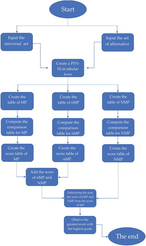
We describe an algorithm for the selection of the alternative in the environment PFN-SS. We have the following 9 steps of the algorithm. The flow chart of of defined algorithm is given in Figure 2.

1. Input $\mathfrak{U}=\left\{{\mathfrak{u}}_1,{\mathfrak{u}}_2,{\mathfrak{u}}_3,\dots ,{\mathfrak{u}}_n\right\}$ as universal set and $\mathfrak{T}=\left\{{\mathcal{t}}_1,{\mathcal{t}}_2,{\mathcal{t}}_3,\dots ,{\mathcal{t}}_m\right\}\subseteq \mathrm{A}$ as a set of attributes.

2. Create a PFN-SS in tabular form.

3. Create the tables of Membership pole (MP), neutral membership pole (nMP), and non-membership pole (NMP).

4. Compute the comparison tables for membership pole, neutral membership pole, and non-membership pole.

5. Create the score tables for membership pole, neutral membership pole, and non-membership pole.

6. Add the scores of neutral membership pole, and non-membership pole.

7. Find out the final score by subtracting the sum of the scores of neutral membership pole, and non-membership pole from the score of membership.

8. Observe the greatest score with the highest grades, if it is in $k-th$ row, then we will select option ${\mathfrak{u}}_k$, $1\le k\le n.$

9. The end.

Figure 2. The flowchart of algorithm defined in Section 4.1.

4.2. Selection of Corona Vaccine

The world is in the midst of a COVID-19 pandemic. A huge number of people are as yet exposed to coronavirus. It’s just the current restrictions that are saving extra people from the deathbed. A vaccine would show our bodies to oppose the infection by preventing us from getting coronavirus or if nothing else making Covid less dangerous. Having a vaccine, alongside better treatments, is the exit strategy. WHO and other medical companies are working on the development of the corona vaccine. Nowadays few medical companies succeed in the development of the corona vaccine. In the following example, we will show that a country can select the best corona vaccine using PFN-SS.

Example 14:

Suppose a country wants to buy a corona vaccine, for this government hires a health expert who will select the best corona vaccine. Let $\mathfrak{U}=\left\{{\mathfrak{u}}_1,{\mathfrak{u}}_2,{\mathfrak{u}}_3,{\mathfrak{u}}_4,{\mathfrak{u}}_5\right\}$ be a set of five corona vaccines which is under consideration of a health expert to buy and $\mathfrak{T}=\left\{{\mathcal{t}}_1,{\mathcal{t}}_2,{\mathcal{t}}_3\right\}$ be a set of attributes, where ${\mathcal{t}}_1$ represents price, ${\mathcal{t}}_2$ represents experimental results of vaccines, and ${\mathcal{t}}_3$ represents delivery time. Based on these attributes, the health expert assigns grades to the corona vaccines in the form of stars which is given in Table 1 in Section 3. The 5-SS is presented in Table 2 of Section 3 and PF5-SS is presented in Table 3 of Section 3.

The tabular form of the MP is given in Table 25.

Table 25. The tabular form of MP in Example 14.

$\mathit{\xi }$	${\mathcal{t}}_1$	${\mathcal{t}}_2$	${\mathcal{t}}_3$
${\mathfrak{u}}_1$	$0.56$	$0.2$	$0.5$
${\mathfrak{u}}_2$	$0.25$	$0.09$	$0.75$
${\mathfrak{u}}_3$	$0.45$	$0.27$	$0.8$
${\mathfrak{u}}_4$	$0.7$	$0.9$	$0.79$
${\mathfrak{u}}_5$	$0.4$	$0.65$	$0.05$

Next, we create the comparison table for MP which is presented in Table 26.

Table 26. The comparison table for MP in Example 14.

$.$	${\mathfrak{u}}_1$	${\mathfrak{u}}_2$	${\mathfrak{u}}_3$	${\mathfrak{u}}_4$	${\mathfrak{u}}_5$
${\mathfrak{u}}_1$	3	2	1	0	2
${\mathfrak{u}}_2$	1	3	1	0	2
${\mathfrak{u}}_3$	2	3	3	1	2
${\mathfrak{u}}_4$	3	3	2	3	3
${\mathfrak{u}}_5$	1	1	1	0	3

After this the membership score for every corona vaccine with the sum of grades $\left(\sum _{\mathcal{i}=1}^5{\mathcal{y}}_{{\mathcal{t}}_{\mathcal{i}}}\right)$ is gotten by subtracting the column sum from the row sum of Table 26. We presented it in Table 27.

Table 27. The score table for MP in Example 14.

	Grade sum $\left(\sum _{\mathcal{i}=1}^5{\mathcal{y}}_{{\mathcal{t}}_{\mathcal{i}}}\right)$	Row sum $\left(\mathit{R}{\mathfrak{s}}_1\right)$	Column sum $\left(\mathit{C}{\mathfrak{s}}_1\right)$	${\mathbf{\Phi }}_1=\mathit{R}{\mathfrak{s}}_1-\mathit{C}{\mathfrak{s}}_1$
${\mathfrak{u}}_1$	6	8	10	−2
${\mathfrak{u}}_2$	4	7	12	−5
${\mathfrak{u}}_3$	7	11	8	3
${\mathfrak{u}}_4$	10	14	4	10
${\mathfrak{u}}_5$	5	6	13	−7

Likewise, the tabular form of the nMP is given in Table 28.

Table 28. The tabular representation of nMP in Example 14.

$\mathit{\delta }$	${\mathcal{t}}_1$	${\mathcal{t}}_2$	${\mathcal{t}}_3$
${\mathfrak{u}}_1$	$0.1$	$0.3$	$0.15$
${\mathfrak{u}}_2$	$0.2$	$0.3$	$0.1$
${\mathfrak{u}}_3$	$0.15$	$0.5$	$0.05$
${\mathfrak{u}}_4$	$0.1$	$0.05$	$0.08$
${\mathfrak{u}}_5$	0.2	0.1	0.4

Next, we create the comparison table for nMP which is presented in Table 29.

Table 29. The comparison table for nMP in Example 14.

$.$	${\mathfrak{u}}_1$	${\mathfrak{u}}_2$	${\mathfrak{u}}_3$	${\mathfrak{u}}_4$	${\mathfrak{u}}_5$
${\mathfrak{u}}_1$	3	2	1	3	1
${\mathfrak{u}}_2$	2	3	2	3	2
${\mathfrak{u}}_3$	2	1	3	2	1
${\mathfrak{u}}_4$	1	0	1	3	0
${\mathfrak{u}}_5$	2	2	2	3	3

After this the neutral membership score for every corona vaccine with the sum of grades $\left(\sum _{\mathcal{i}=1}^5{\mathcal{y}}_{{\mathcal{t}}_{\mathcal{i}}}\right)$ is gotten by subtracting the column sum from the row sum of Table 29. We presented it in Table 30.

Table 30. The score table for nMP in Example 14.

	Grade sum $\left(\sum _{\mathcal{i}=1}^5{\mathcal{y}}_{{\mathcal{t}}_{\mathcal{i}}}\right)$	Row sum $\left(\mathit{R}{\mathfrak{s}}_2\right)$	Column sum $\left(\mathit{C}{\mathfrak{s}}_2\right)$	${\mathbf{\Phi }}_2=\mathit{R}{\mathfrak{s}}_2-\mathit{C}{\mathfrak{s}}_2$
${\mathfrak{u}}_1$	6	10	10	0
${\mathfrak{u}}_2$	4	12	8	4
${\mathfrak{u}}_3$	7	9	9	0
${\mathfrak{u}}_4$	10	5	14	−9
${\mathfrak{u}}_5$	5	12	7	5

Similarly, now the tabular form of the NMP is given in Table 31.

Table 31. The tabular representation of NMP in Example 14.

$\vartheta$	${\mathcal{t}}_1$	${\mathcal{t}}_2$	${\mathcal{t}}_3$
${\mathfrak{u}}_1$	$0.2$	$0.4$	$0.3$
${\mathfrak{u}}_2$	$0.5$	$0.5$	$0.1$
${\mathfrak{u}}_3$	$0.3$	$0.1$	$0.1$
${\mathfrak{u}}_4$	$0.1$	$0.04$	$0.05$
${\mathfrak{u}}_5$	$0.3$	$0.15$	$0.5$

Next, we create the comparison table for NMP which is presented in Table 32.

Table 32. The comparison table for NMP in Example 14.

$.$	${\mathfrak{u}}_1$	${\mathfrak{u}}_2$	${\mathfrak{u}}_3$	${\mathfrak{u}}_4$	${\mathfrak{u}}_5$
${\mathfrak{u}}_1$	3	1	2	3	2
${\mathfrak{u}}_2$	2	3	3	3	2
${\mathfrak{u}}_3$	1	1	3	3	1
${\mathfrak{u}}_4$	0	0	0	3	0
${\mathfrak{u}}_5$	2	1	3	3	3

After this the non-membership score for every corona vaccine with the sum of grades $\left(\sum _{\mathcal{i}=1}^5{\mathcal{y}}_{{\mathcal{t}}_{\mathcal{i}}}\right)$ is gotten by subtracting the column sum from the row sum of Table 32. We presented it in Table 33.

Table 33. The score table for NMP in Example 14.

	Grade sum $\left(\sum _{\mathcal{i}=1}^5{\mathcal{y}}_{{\mathcal{t}}_{\mathcal{i}}}\right)$	Row sum $\left(\mathit{R}{\mathfrak{s}}_3\right)$	Column sum $\left(\mathit{C}{\mathfrak{s}}_3\right)$	${\mathbf{\Phi }}_3=\mathit{R}{\mathfrak{s}}_3-\mathit{C}{\mathfrak{s}}_3$
${\mathfrak{u}}_1$	6	11	8	3
${\mathfrak{u}}_2$	4	13	6	7
${\mathfrak{u}}_3$	7	9	11	−2
${\mathfrak{u}}_4$	10	3	15	−12
${\mathfrak{u}}_5$	5	12	8	4

Finally, we add the scores of neutral membership and non-membership and then subtract it by the score of membership as presented in Table 35. In Table 34, we show the addition of scores of neutral membership and non-membership.

Table 34. Add the score of nMP given in table (30) and NMP given in Table 33.

	Grade sum $\left(\sum _{\mathcal{i}=1}^5{\mathcal{y}}_{{\mathcal{t}}_{\mathcal{i}}}\right)$	${\mathbf{\Phi }}_2$	${\mathbf{\Phi }}_3$	${\mathbf{\Phi }}_4={\mathbf{\Phi }}_2+{\mathbf{\Phi }}_3$
${\mathfrak{u}}_1$	$6$	$0$	$3$	$3$
${\mathfrak{u}}_2$	$4$	$4$	$7$	$11$
${\mathfrak{u}}_3$	$7$	$0$	$-2$	$-2$
${\mathfrak{u}}_4$	$10$	$-9$	$-12$	$-21$
${\mathfrak{u}}_5$	$5$	$5$	$4$	$9$

Table 35. Table of final score with grades linked with PF5-SS of Example 14.

	Grade sum $\left(\sum _{\mathcal{i}=1}^5{\mathcal{y}}_{{\mathcal{t}}_{\mathcal{i}}}\right)$	${\mathbf{\Phi }}_1$	${\mathbf{\Phi }}_4$	FINAL SCORE $={\mathbf{\Phi }}_1-{\mathbf{\Phi }}_4$
${\mathfrak{u}}_1$	$6$	$-2$	$3$	$1$
${\mathfrak{u}}_2$	$4$	$-5$	$11$	$-16$
${\mathfrak{u}}_3$	$7$	$3$	$-2$	$5$
${\mathfrak{u}}_4$	$10$	$10$	$-21$	$31$
${\mathfrak{u}}_5$	$5$	$-7$	$9$	$-16$

The corona vaccine ${\mathfrak{u}}_4$ has highest grades with the greatest score so the health expert wants to buy the corona vaccine ${\mathfrak{u}}_4$ for his country. He thinks that ${\mathfrak{u}}_4$ is the best corona vaccine among the present 5 corona vaccines which can save more people from the corona.

4.3. Selection of a Next Generation Firewall (NGFW)

The firewall refers to a security gateway that protects the computer networks from malicious instructions. There are several kinds of firewalls in the market and every firewall has its benefits and disbenefits. Therefore, how to select a beneficial firewall by seeing its effectiveness and precision is a conventional multi-attribute DM (MADM) problem.

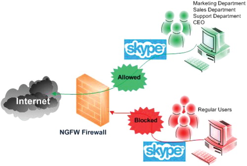
Chances are you have probably heard or read about next generation firewalls, it seems like everyone is talking about what a great innovation it is in the network security market. Traditional firewalls are becoming less capable of adequately protecting enterprise wireless networks with the rapid evolution of applications and threats. Instead of a completely new approach to wireless network security, the traditional firewall has been transformed into next generation firewall to restore application visibility and control and regain the advantage in protecting the enterprise wireless networks. See Figure 3.

Figure 3. The next generation firewall.

In this article, we discussed that a company wants to purchase a next generation firewall whose details are given in Example 2 Section 3. Below in Example 15 we will reconsider Example 2 to get the result.

Example 15:

A multi-national company wants to enhance the security of its wireless network. The company plans to buy the next generation firewall for blocking illegal access. For that, the company hire an expert and provide him four next generation firewalls, i.e. $\mathfrak{U}=\left\{{\mathfrak{u}}_1,{\mathfrak{u}}_2,{\mathfrak{u}}_3,{\mathfrak{u}}_4\right\}$. The expert have to finalise one of the best next generation firewalls in these four firewalls based on the three given attributes $\mathfrak{T}=\left\{{\mathcal{t}}_1,{\mathcal{t}}_2,{\mathcal{t}}_3\right\}$, where ${\mathcal{t}}_1$ represents scan for viruses and malware in allowed collaborative applications, ${\mathcal{t}}_2$ represents identify and control applications sharing the same connection, and ${\mathcal{t}}_3$ represents decrypt outbound SSL. Based on these attributes the expert assigns grades to given four next generation firewalls in the form of stars. A 3-soft set can be obtained from Table 36, where three stars are for ‘very good', two stars are for ‘good', one star is for ‘normal', a hole is for ‘poor'.

Table 36. Information obtained from associated data.

$\mathfrak{U}$	${\mathcal{t}}_1$	${\mathcal{t}}_2$	${\mathcal{t}}_3$
${\mathfrak{u}}_1$	$◻$	$\star \star$	$\star \star \star$
${\mathfrak{u}}_2$	$\star \star$	$\star \star \star$	$\star \star$
${\mathfrak{u}}_3$	$\star \star$	$\star \star \star$	$\star$
${\mathfrak{u}}_4$	$◻$	$\star \star$	$\star \star$

The set $\mathcal{Y}=\left\{0,1,2,3\right\}$ can be associated with the stars given in Table 36, where 3 represents ${}^{\prime }\star \star {\star }^{\prime }$, 2 represents ${}^{\prime }\star {\star }^{\prime }$, 1 represents ${}^{\prime }{\star }^{\prime }$, and 0 represents ${}^{\prime }{◻}^{\prime }$. The 4-SS $\left(\mathrm{I},\mathfrak{T},4\right)$ is given as follows: $\mathrm{I}\left({\mathcal{t}}_1\right)=\left\{\left({\mathfrak{u}}_1,0\right),\left({\mathfrak{u}}_2,2\right),\left({\mathfrak{u}}_3,2\right),\left({\mathfrak{u}}_4,0\right)\right\}$ $\mathrm{I}\left({\mathcal{t}}_2\right)=\left\{\left({\mathfrak{u}}_1,2\right),\left({\mathfrak{u}}_2,3\right),\left({\mathfrak{u}}_3,3\right),\left({\mathfrak{u}}_4,2\right)\right\}$ $\mathrm{I}\left({\mathcal{t}}_3\right)=\left\{\left({\mathfrak{u}}_1,3\right),\left({\mathfrak{u}}_2,2\right),\left({\mathfrak{u}}_3,1\right),\left({\mathfrak{u}}_4,2\right)\right\}$

The tabular form of 4-SS is interpreted in Table 37.

The membership $\left(\xi \right)$, neutral $\left(\delta \right)$, and non-membership $\left(\vartheta \right)$ follow the following grading criteria. For all $\mathfrak{u}\in \mathfrak{U},0\le \xi \left(\mathfrak{u}\right)+\delta \left(\mathfrak{u}\right)+\vartheta \left(\mathfrak{u}\right)\le 1$, where $0\le \delta \left(\mathfrak{u}\right),\vartheta \left(\mathfrak{u}\right)\le 1$. We allot grade 0 if $0\le \xi \left(\mathfrak{u}\right)<0.25$. Similarly $\mathrm{\forall }\mathfrak{u}\in \mathfrak{U}$ we relate: grade 1 if $0.25\le \xi \left(\mathfrak{u}\right)<0.5$, grade 2, if $0.5\le \xi \left(\mathfrak{u}\right)<0.75,\text{grade }3,\text{ if }0.75\le \xi \left(\mathfrak{u}\right)<\mathrm{1.0.}$ Then by Definition 14, the PF5-SS is given as follows: $\mathrm{Y}\left({\mathcal{t}}_1\right)=\left\{\begin{array}{c}\left(\left({\mathfrak{u}}_1,0\right),0.16,0.4,0.1\right),\left(\left({\mathfrak{u}}_2,2\right),0.65,0.1,0.15\right),\left(\left({\mathfrak{u}}_3,2\right),0.55,0.25,0.05\right),\\ \left(\left({\mathfrak{u}}_4,0\right),0.1,0.4,0.4\right)\end{array}\right\}$ $\mathrm{Y}\left({\mathcal{t}}_2\right)=\left\{\begin{array}{c}\left(\left({\mathfrak{u}}_1,2\right),0.6,0.2,0.11\right),\left(\left({\mathfrak{u}}_2,3\right),0.8,0.13,0.05\right),\left(\left({\mathfrak{u}}_3,3\right),0.9,0.05,0.01\right),\\ \left(\left({\mathfrak{u}}_4,2\right),0.71,0.1,0.0\right)\end{array}\right\}$ $\mathrm{Y}\left({\mathcal{t}}_3\right)=\left\{\begin{array}{c}\left(\left({\mathfrak{u}}_1,3\right),0.88,0.05,0.03\right),\left(\left({\mathfrak{u}}_2,2\right),0.58,0.3,0.1\right),\left(\left({\mathfrak{u}}_3,1\right),0.4,0.2,0.4\right),\\ \left(\left({\mathfrak{u}}_4,2\right),0.7,0.05,0.2\right)\end{array}\right\}$

Table 37. The tabular form of 4-SS.

$\left(\mathbf{I},\mathfrak{T},5\right)$	${\mathcal{t}}_1$	${\mathcal{t}}_2$	${\mathcal{t}}_3$
${\mathfrak{u}}_1$	$0$	$2$	$3$
${\mathfrak{u}}_2$	$2$	$3$	$2$
${\mathfrak{u}}_3$	$2$	$3$	$1$
${\mathfrak{u}}_4$	$0$	$2$	$2$

Clearly, the PF5-SS can be described in the tabular form given in Table 38.

The tabular form of the MP is given in Table 39.

Table 38. The tabular representation of the picture fuzzy 4-soft set in Example 15.

$\left(\mathit{Y},\left(\mathbf{I},\mathfrak{T},4\right)\right)$	${\mathcal{t}}_1$	${\mathcal{t}}_2$	${\mathcal{t}}_3$
${\mathfrak{u}}_1$	$0,\left(0.16,0.4,0.1\right)$	$2,\left(0.6,0.2,0.11\right)$	$3,\left(0.88,0.05,0.03\right)$
${\mathfrak{u}}_2$	$2,\left(0.65,0.1,0.15\right)$	$3,\left(0.8,0.13,0.05\right)$	$2,\left(0.58,0.3,0.1\right)$
${\mathfrak{u}}_3$	$2,\left(0.65,0.25,0.05\right)$	$3,\left(0.9,0.05,0.01\right)$	$1,\left(0.4,0.2,0.4\right)$
${\mathfrak{u}}_4$	$0,\left(0.1,0.4,0.4\right)$	$2,\left(0.7,0.1,0.0\right)$	$2,\left(0.7,0.05,0.2\right)$

Table 39. The tabular form of MP Example 15.

$\mathit{\xi }$	${\mathcal{t}}_1$	${\mathcal{t}}_2$	${\mathcal{t}}_3$
${\mathfrak{u}}_1$	$0.16$	$0.6$	$0.88$
${\mathfrak{u}}_2$	$0.65$	$0.8$	$0.58$
${\mathfrak{u}}_3$	$0.65$	$0.9$	$0.4$
${\mathfrak{u}}_4$	$0.1$	$0.7$	$0.7$

Next, we create the comparison table for MP which is presented in Table 40.

Table 40. The comparison table for MP in Example 15.

$.$	${\mathfrak{u}}_1$	${\mathfrak{u}}_2$	${\mathfrak{u}}_3$	${\mathfrak{u}}_4$
${\mathfrak{u}}_1$	$3$	$1$	$1$	$3$
${\mathfrak{u}}_2$	$2$	$3$	$2$	$2$
${\mathfrak{u}}_3$	$2$	$2$	$3$	$2$
${\mathfrak{u}}_4$	$1$	$1$	$1$	$3$

After this the membership score for every firewall with the sum of grades $\left(\sum _{\mathcal{i}=1}^4{\mathcal{y}}_{{\mathcal{t}}_{\mathcal{i}}}\right)$ is gotten by subtracting the column sum from the row sum of Table 40. We presented it in the Table 38 (Table 41).

Table 41. The score table for MP in Example 15.

	Grade sum $\left(\sum _{\mathcal{i}=1}^4{\mathcal{y}}_{{\mathcal{t}}_{\mathcal{i}}}\right)$	Row sum $\left(\mathit{R}{\mathfrak{s}}_1\right)$	Column sum $\left(\mathit{C}{\mathfrak{s}}_1\right)$	${\mathbf{\Phi }}_1=\mathit{R}{\mathfrak{s}}_1-\mathit{C}{\mathfrak{s}}_1$
${\mathfrak{u}}_1$	$5$	$8$	$8$	$0$
${\mathfrak{u}}_2$	$7$	$9$	$7$	$2$
${\mathfrak{u}}_3$	$6$	$9$	$7$	$2$
${\mathfrak{u}}_4$	$4$	$6$	$10$	$-4$

Likewise, the tabular form of the nMP is given in Table 42.

Table 42. The tabular representation of nMP in Example 15.

$\mathit{\delta }$	${\mathcal{t}}_1$	${\mathcal{t}}_2$	${\mathcal{t}}_3$
${\mathfrak{u}}_1$	$0.4$	$0.2$	$0.05$
${\mathfrak{u}}_2$	$0.1$	$0.13$	$0.3$
${\mathfrak{u}}_3$	$0.25$	$0.05$	$0.2$
${\mathfrak{u}}_4$	$0.4$	$0.1$	$0.05$

Next, we create the comparison table for nMP which is presented in Table 43.

Table 43. The comparison table for nMP in Example 15.

$.$	${\mathfrak{u}}_1$	${\mathfrak{u}}_2$	${\mathfrak{u}}_3$	${\mathfrak{u}}_4$
${\mathfrak{u}}_1$	$3$	$2$	$2$	$3$
${\mathfrak{u}}_2$	$1$	$3$	$2$	$2$
${\mathfrak{u}}_3$	$1$	$1$	$3$	$1$
${\mathfrak{u}}_4$	$2$	$1$	$2$	$3$

After this the neutral membership score for every firewall with the sum of grades $\left(\sum _{\mathcal{i}=1}^4{\mathcal{y}}_{{\mathcal{t}}_{\mathcal{i}}}\right)$ is gotten by subtracting the column sum from the row sum of Table 43. We presented it in Table 44.

Table 44. The score table for nMP in Example 15.

	Grade sum $\left(\sum _{\mathcal{i}=1}^4{\mathcal{y}}_{{\mathcal{t}}_{\mathcal{i}}}\right)$	Row sum $\left(\mathit{R}{\mathfrak{s}}_2\right)$	Column sum $\left(\mathit{C}{\mathfrak{s}}_2\right)$	${\mathbf{\Phi }}_2=\mathit{R}{\mathfrak{s}}_2-\mathit{C}{\mathfrak{s}}_2$
${\mathfrak{u}}_1$	$5$	$10$	$7$	$3$
${\mathfrak{u}}_2$	$7$	$8$	$7$	$1$
${\mathfrak{u}}_3$	$6$	$6$	$9$	$-3$
${\mathfrak{u}}_4$	$4$	$8$	$9$	$-1$

Similarly, now the tabular form of the NMP is given in Table 45.

Table 45. The tabular representation of NMP in Example 15.

$\vartheta$	${\mathcal{t}}_1$	${\mathcal{t}}_2$	${\mathcal{t}}_3$
${\mathfrak{u}}_1$	$0.1$	$0.11$	$0.03$
${\mathfrak{u}}_2$	$0.15$	$0.05$	$0.1$
${\mathfrak{u}}_3$	$0.05$	$0.01$	$0.4$
${\mathfrak{u}}_4$	$0.4$	$0.0$	$0.2$

Next we create the comparison table for NMP which is presented in Table 46.

Table 46. The comparison table for NMP in Example 15.

$.$	${\mathfrak{u}}_1$	${\mathfrak{u}}_2$	${\mathfrak{u}}_3$	${\mathfrak{u}}_4$
${\mathfrak{u}}_1$	$3$	$1$	$2$	$1$
${\mathfrak{u}}_2$	$2$	$3$	$2$	$1$
${\mathfrak{u}}_3$	$1$	$1$	$3$	$2$
${\mathfrak{u}}_4$	$2$	$2$	$1$	$3$

After this the non-membership score for every firewall with the sum of grades $\left(\sum _{\mathcal{i}=1}^4{\mathcal{y}}_{{\mathcal{t}}_{\mathcal{i}}}\right)$ is gotten by subtracting the column sum from the row sum of Table 46. We presented it in Table 47.

Table 47. The score table for NMP in Example 15.

	Grade sum $\left(\sum _{\mathcal{i}=1}^4{\mathcal{y}}_{{\mathcal{t}}_{\mathcal{i}}}\right)$	Row sum $\left(\mathit{R}{\mathfrak{s}}_3\right)$	Column sum $\left(\mathit{C}{\mathfrak{s}}_3\right)$	${\mathbf{\Phi }}_3=\mathit{R}{\mathfrak{s}}_3-\mathit{C}{\mathfrak{s}}_3$
${\mathfrak{u}}_1$	$5$	$7$	$7$	$0$
${\mathfrak{u}}_2$	$7$	$8$	$7$	$1$
${\mathfrak{u}}_3$	$6$	$7$	$8$	$-1$
${\mathfrak{u}}_4$	$4$	$8$	$7$	$1$

Finally, we add the scores of neutral membership and non-membership and then subtract it by the score of membership as presented in Table 49. In Table 48 we show the addition of scores of neutral membership and non-membership.

Table 48. Add the score of nMP given in table (44) and NMP given in Table 47.

	Grade sum $\left(\sum _{\mathcal{i}=1}^4{\mathcal{y}}_{{\mathcal{t}}_{\mathcal{i}}}\right)$	${\mathbf{\Phi }}_2$	${\mathbf{\Phi }}_3$	${\mathbf{\Phi }}_4={\mathbf{\Phi }}_2+{\mathbf{\Phi }}_3$
${\mathfrak{u}}_1$	$5$	$3$	$0$	$3$
${\mathfrak{u}}_2$	$7$	$1$	$1$	$2$
${\mathfrak{u}}_3$	$6$	$-3$	$-1$	$-4$
${\mathfrak{u}}_4$	$4$	$-1$	$1$	$0$

Table 49. Table of final score with grades linked with PF6-SS of Example 15.

	Grade sum $\left(\sum _{\mathcal{i}=1}^4{\mathcal{y}}_{{\mathcal{t}}_{\mathcal{i}}}\right)$	${\mathbf{\Phi }}_1$	${\mathbf{\Phi }}_4$	FINAL SCORE $={\mathbf{\Phi }}_1-{\mathbf{\Phi }}_4$
${\mathfrak{u}}_1$	$5$	$0$	$3$	$-3$
${\mathfrak{u}}_2$	$7$	$2$	$2$	$0$
${\mathfrak{u}}_3$	$6$	$2$	$-4$	$6$
${\mathfrak{u}}_4$	$4$	$-4$	$0$	$-4$

The firewall ${\mathfrak{u}}_3$ has the greatest score so the expert wants to prefer the firewall ${\mathfrak{u}}_1$ to the company to purchase.

5. Comparison

In this segment, we will compare our presented work PFN-SS with IFN-SS. By the following, we will show that the PFN-SS is more general and more effective than the IFN-SS.

Example 16:

An expert wants to give his opinion about the presidential election of America. Let there are 3 presidential candidates in the election, i.e. $\mathfrak{U}=\left\{{\mathfrak{u}}_1,{\mathfrak{u}}_2,{\mathfrak{u}}_3\right\}$, and $\mathfrak{T}=\left\{{\mathcal{t}}_1,{\mathcal{t}}_2,{\mathcal{t}}_3\right\}$ be a set of attributes, where ${\mathcal{t}}_1$ represents experience, ${\mathcal{t}}_2$ represents working abilities, and ${\mathcal{t}}_3$ future vision. An expert gives them grades based on these attributes in the shape of stars which is presented in Table 50. Where Four stars are for ‘Excellent', three stars are for ‘very good', two stars are for ‘good', one star is for ‘normal', a hole is for ‘poor’.

Table 50. Information obtained from the associated data.

	${\mathcal{t}}_1$	${\mathcal{t}}_2$	${\mathcal{t}}_3$
${\mathfrak{u}}_1$	$\star \star \star \star$	$\star \star \star$	$\star \star \star \star$
${\mathfrak{u}}_2$	$\star \star \star$	$\star \star \star \star$	$\star \star \star \star$
${\mathfrak{u}}_3$	$\star$	$◻$	$\star \star \star \star$

The set $\mathcal{Y}=\left\{0,1,2,3,4\right\}$ can be associated with the stars given in Table 50, where 4 represents ${}^{\prime }\star \star \star {\star }^{\prime }$, 3 represents ${}^{\prime }\star \star {\star }^{\prime }$, 2 represents ${}^{\prime }\star {\star }^{\prime }$, 1 represents ${}^{\prime }{\star }^{\prime }$, and 0 represents ${}^{\prime }{◻}^{\prime }$. The 5-SS $\left(\mathrm{I},\mathfrak{T},5\right)$ is given as follows: $\mathrm{I}\left({\mathcal{t}}_1\right)=\left\{\left({\mathfrak{u}}_1,4\right),\left({\mathfrak{u}}_2,3\right),\left({\mathfrak{u}}_3,1\right)\right\}$ $\mathrm{I}\left({\mathcal{t}}_2\right)=\left\{\left({\mathfrak{u}}_1,3\right),\left({\mathfrak{u}}_2,4\right),\left({\mathfrak{u}}_3,0\right),\right\}$ $\mathrm{I}\left({\mathcal{t}}_3\right)=\left\{\left({\mathfrak{u}}_1,4\right),\left({\mathfrak{u}}_2,4\right),\left({\mathfrak{u}}_3,4\right),\right\}$

The tabular form of 5-SS is interpreted in Table 51.

An expert link an IFN with each of the grade given by his self. In the result, he will get IF5-SS which is presented in Table 49 (Table 52).

Table 51. The tabular form of 5-SS.

$\left(\mathbf{I},\mathfrak{T},5\right)$	${\mathcal{t}}_1$	${\mathcal{t}}_2$	${\mathcal{t}}_3$
${\mathfrak{u}}_1$	$4$	$3$	$4$
${\mathfrak{u}}_2$	$3$	$4$	$4$
${\mathfrak{u}}_3$	$1$	$0$	$4$

Table 52. The tabular representation of IF5-SS $\left(\mathbf{K},\left(\mathbf{I},\mathfrak{T},5\right)\right)$ in Example 16.

$\left(\mathbf{K},\left(\mathbf{I},\mathfrak{T},5\right)\right)$	${\mathcal{t}}_1$	${\mathcal{t}}_2$	${\mathcal{t}}_3$
${\mathfrak{u}}_1$	$4,\left(0.9,0.04\right)$	$3,\left(075,0.1\right)$	$4,\left(0.85,0.1\right)$
${\mathfrak{u}}_2$	$3,\left(0.75,0.2\right)$	$4,\left(0.87,0.08\right)$	$4,\left(0.89,0.04\right)$
${\mathfrak{u}}_3$	$1,\left(0.25,0.5\right)$	$0,\left(0.13,0.4\right)$	$4,\left(0.9,0.04\right)$

To explain this more we consider the cell in the 1st row and 3rd column, i.e. $3,\left(0.75,0.1\right)$, where 3 is the grade given by the expert to the candidate ${\mathfrak{u}}_1$ on his working ability, $0.75$ be the grade of membership which is given by the expert to the candidate ${\mathfrak{u}}_1$ based on his working ability and 0.1 is the grade of non-membership given to the candidate ${\mathfrak{u}}_1$ by the expert.

Now we will use the algorithm defined for IFN-SS by Akram et al. [46] to find which candidate will win the election in the expert’s opinion. The tabular form of MP is described in Table 53. We create the comparison table for MP which is presented in Table 54. After this the membership score for every presidential candidate with the sum of grades $\left(\sum _{\mathcal{i}=1}^3{\mathcal{y}}_{{\mathcal{t}}_{\mathcal{i}}}\right)$ is gotten by subtracting the column sum from the row sum of Table 54. We presented it in Table 55.

Table 53. The tabular representation of MP Example 16.

$\mathit{\xi }$	${\mathcal{t}}_1$	${\mathcal{t}}_2$	${\mathcal{t}}_3$
${\mathfrak{u}}_1$	$0.9$	$0.75$	$0.85$
${\mathfrak{u}}_2$	$0.75$	$0.87$	$0.89$
${\mathfrak{u}}_3$	$0.25$	$0.13$	$0.9$

Table 54. The comparison table for MP in Example 16.

$.$	${\mathfrak{u}}_1$	${\mathfrak{u}}_2$	${\mathfrak{u}}_3$
${\mathfrak{u}}_1$	$3$	$1$	$2$
${\mathfrak{u}}_2$	$2$	$3$	$2$
${\mathfrak{u}}_3$	$1$	$1$	$3$

Table 55. The score table for MP in Example 16.

	Grade sum $\left(\sum _{\mathcal{i}=1}^3{\mathcal{y}}_{{\mathcal{t}}_{\mathcal{i}}}\right)$	Row sum $\left(\mathit{R}{\mathfrak{s}}_1\right)$	Column sum $\left(\mathit{C}{\mathfrak{s}}_1\right)$	${\mathbf{\Phi }}_1=\mathit{R}{\mathfrak{s}}_1-\mathit{C}{\mathfrak{s}}_1$
${\mathfrak{u}}_1$	$11$	$6$	$6$	$0$
${\mathfrak{u}}_2$	$11$	$7$	$5$	$2$
${\mathfrak{u}}_3$	$5$	$5$	$7$	$-2$

Similarly, now the tabular form of the NMP is given in Table 56. We create the comparison table for NMP which is presented in Table 57. After this the non-membership score for a presidential candidate with the sum of grades $\left(\sum _{\mathcal{i}=1}^3{\mathcal{y}}_{{\mathcal{t}}_{\mathcal{i}}}\right)$ is gotten by subtracting the column sum from the row sum of Table 57. We presented it in the Table 58.

Table 56. The tabular representation of NMP in Example 16.

$\vartheta$	${\mathcal{t}}_1$	${\mathcal{t}}_2$	${\mathcal{t}}_3$
${\mathfrak{u}}_1$	$0.04$	$0.1$	$0.1$
${\mathfrak{u}}_2$	$0.2$	$0.08$	$0.04$
${\mathfrak{u}}_3$	$0.5$	$0.4$	$0.04$

Table 57. The comparison table for NMP in Example 16.

$.$	${\mathfrak{u}}_1$	${\mathfrak{u}}_2$	${\mathfrak{u}}_3$
${\mathfrak{u}}_1$	$3$	$2$	$1$
${\mathfrak{u}}_2$	$1$	$3$	$1$
${\mathfrak{u}}_3$	$2$	$3$	$3$

Table 58. The score table for NMP in Example 16.

	Grade sum $\left(\sum _{\mathcal{i}=1}^3{\mathcal{y}}_{{\mathcal{t}}_{\mathcal{i}}}\right)$	Row sum $\left(\mathit{R}{\mathfrak{s}}_3\right)$	Column sum $\left(\mathit{C}{\mathfrak{s}}_3\right)$	${\mathbf{\Phi }}_3=\mathit{R}{\mathfrak{s}}_3-\mathit{C}{\mathfrak{s}}_3$
${\mathfrak{u}}_1$	$11$	$6$	$6$	$0$
${\mathfrak{u}}_2$	$11$	$5$	$8$	$-3$
${\mathfrak{u}}_3$	$5$	$8$	$5$	$3$

Finally, we subtract the score of non-membership by the membership which is described in Table 59.

Table 59. Table of final score with grades linked with IF5-SS of Example 16.

	Grade sum $\left(\sum _{\mathcal{i}=1}^3{\mathcal{y}}_{{\mathcal{t}}_{\mathcal{i}}}\right)$	${\mathbf{\Phi }}_1$	${\mathbf{\Phi }}_3$	FINAL SCORE $={\mathbf{\Phi }}_1-{\mathbf{\Phi }}_3$
${\mathfrak{u}}_1$	$11$	$0$	$0$	$0$
${\mathfrak{u}}_2$	$11$	$2$	$-3$	$5$
${\mathfrak{u}}_3$	$5$	$-2$	$3$	$-5$

According to the algorithm defined by Akram et al. [46], the expert found that presidential candidate ${\mathfrak{u}}_2$ has highest grades with the greatest score so he thinks ${\mathfrak{u}}_2$ will the next president of America.

Later the expert realised that in this DM, he forgot to count the grade of neutral membership. Now he wants to add the grade of neutral membership in this DM because he knows that the voters may be categorised into 4 groups, i.e. vote for, abstains, vote against, and refusal of the voting. In the above DM, he has no abstain so now he wants to add this in this DM to get a more accurate and exact result. But he can’t add this grade of neutral membership in the environment of IFN-SS. IFN-SS is unable to solve such data. To get the result the expert will use PFN-SS. Reconsider Example 15, The expert will link a PFN to every grade given in Table 51. As a result, he will get PF5-SS which is presented in Table 60.

Table 60. The tabular form of PF5-SS of Example 16.

$\left(\mathit{Y},\left(\mathbf{I},\mathfrak{T},5\right)\right)$	${\mathcal{t}}_1$	${\mathcal{t}}_2$	${\mathcal{t}}_3$
${\mathfrak{u}}_1$	$4,\left(0.9,0.05,0.04\right)$	$3,\left(075,0.01,0.1\right)$	$4,\left(0.85,0.04,0.1\right)$
${\mathfrak{u}}_2$	$3,\left(0.75,0.09,0.2\right)$	$4,\left(0.87,0.04,0.08\right)$	$4,\left(0.89,0.06,0.04\right)$
${\mathfrak{u}}_3$	$1,\left(0.25,0.08,0.5\right)$	$0,\left(0.13,0.03,0.4\right)$	$4,\left(0.9,0.05,0.04\right)$

To explain this more we consider the cell in the 1st row and 3rd column, i.e. $3,\left(0.75,0.01,0.1\right)$, where 3 is the grade given by the expert to the candidate ${\mathfrak{u}}_1$ on his working ability, $0.75$ be the grade of membership which is given by the expert to the candidate ${\mathfrak{u}}_1$ based on his working ability, $0.01$ is the grade of neutral membership, and 0.1 is the grade of non-membership given to the candidate ${\mathfrak{u}}_1$ by the expert.

Now we will use the algorithm defined in Section 4 of this article to find that which candidate will win the election in the expert’s opinion. The tabular form of MP is described in Table 61. We create the comparison table for MP which is presented in Table 62. After this the membership score for every presidential candidate with the sum of grades $\left(\sum _{\mathcal{i}=1}^3{\mathcal{y}}_{{\mathcal{t}}_{\mathcal{i}}}\right)$ is gotten by subtracting the column sum from the row sum of Table 62. We presented it in Table 63.

Table 61. The tabular representation of MP in Example 16.

$\mathit{\xi }$	${\mathcal{t}}_1$	${\mathcal{t}}_2$	${\mathcal{t}}_3$
${\mathfrak{u}}_1$	$0.9$	$0.75$	$0.85$
${\mathfrak{u}}_2$	0.75	0.87	0.89
${\mathfrak{u}}_3$	0.25	0.13	0.9

Table 62. The comparison table for MP in Example 16.

.	${\mathfrak{u}}_1$	${\mathfrak{u}}_2$
${\mathfrak{u}}_1$	3	1	2
${\mathfrak{u}}_2$	2	3	2
${\mathfrak{u}}_3$	1	1	3

Table 63. The score table for MP in Example 16.

	Grade sum $\left(\sum _{\mathcal{i}=1}^3{\mathcal{y}}_{{\mathcal{t}}_{\mathcal{i}}}\right)$	Row sum $\left(\mathit{R}{\mathfrak{s}}_1\right)$	Column sum $\left(\mathit{C}{\mathfrak{s}}_1\right)$	${\mathbf{\Phi }}_1=\mathit{R}{\mathfrak{s}}_1-\mathit{C}{\mathfrak{s}}_1$
${\mathfrak{u}}_1$	11	6	6	0
${\mathfrak{u}}_2$	11	7	5	2
${\mathfrak{u}}_3$	5	5	7	−2

Likewise, the tabular form of the nMP is given in Table 64.We create the comparison table for nMP which is presented in Table 65. After this the neutral membership score for every presidential candidate with the sum of grades $\left(\sum _{\mathcal{i}=1}^3{\mathcal{y}}_{{\mathcal{t}}_{\mathcal{i}}}\right)$ is gotten by subtracting the column sum from the row sum of Table 65. We presented it in Table 66.

Table 64. The tabular form of nMP is given in Example 16.

$\mathit{\delta }$	${\mathfrak{t}}_1$	${\mathfrak{t}}_1$	${\mathfrak{t}}_1$
${\mathfrak{u}}_1$	0.05	0.01	0.045
${\mathfrak{u}}_2$	0.09	0.04	0.06
${\mathfrak{u}}_3$	0.08	0.03	0.05

Table 65. The comparison table for nMP in Example 16.

.	${\mathfrak{u}}_1$	${\mathfrak{u}}_2$	${\mathfrak{u}}_3$
${\mathfrak{u}}_1$	3	0	0
${\mathfrak{u}}_2$	3	3	3
${\mathfrak{u}}_3$	3	0	3

Table 66. The score table for nMP in Example 16.

	Grade sum $\left(\sum _{\mathcal{i}=1}^3{\mathcal{y}}_{{\mathcal{t}}_{\mathcal{i}}}\right)$	Row sum $\left(\mathit{R}{\mathfrak{s}}_2\right)$	Column sum $\left(\mathit{C}{\mathfrak{s}}_2\right)$	${\mathbf{\Phi }}_2=\mathit{R}{\mathfrak{s}}_2-\mathit{C}{\mathfrak{s}}_2$
${\mathfrak{u}}_1$	11	3	9	−6
${\mathfrak{u}}_2$	11	9	3	6
${\mathfrak{u}}_3$	5	6	6	0

Similarly, now the tabular form of the NMP is given in Table 67. We create the comparison table for NMP which is presented in Table 68. After this the non-membership score for a presidential candidate with the sum of grades $\left(\sum _{\mathcal{i}=1}^3{\mathcal{y}}_{{\mathcal{t}}_{\mathcal{i}}}\right)$ is gotten by subtracting the column sum from the row sum of Table 68. We presented it in Table 69.

Table 67. The tabular form of NMP given in Example 16.

$\vartheta$	${\mathcal{t}}_1$	${\mathcal{t}}_2$	${\mathcal{t}}_3$
${\mathfrak{u}}_1$	0.04	0.1	0.1
${\mathfrak{u}}_2$	0.2	0.08	0.04
${\mathfrak{u}}_3$	0.5	0.4	0.04

Table 68. The comparison table for NMP in Example 16.

.	${\mathfrak{u}}_1$	${\mathfrak{u}}_2$	${\mathfrak{u}}_3$
${\mathfrak{u}}_1$	3	2	1
${\mathfrak{u}}_2$	1	3	1
${\mathfrak{u}}_3$	2	3	3

Table 69. The score table for NMP in Example 16.

	Grade sum $\left(\sum _{\mathcal{i}=1}^3{\mathcal{y}}_{{\mathcal{t}}_{\mathcal{i}}}\right)$	Row sum $\left(\mathit{R}{\mathfrak{s}}_3\right)$	Column sum $\left(\mathit{C}{\mathfrak{s}}_3\right)$	${\mathbf{\Phi }}_3=\mathit{R}{\mathfrak{s}}_3-\mathit{C}{\mathfrak{s}}_3$
${\mathfrak{u}}_1$	11	6	6	0
${\mathfrak{u}}_2$	11	5	8	−3
${\mathfrak{u}}_3$	5	8	5	−3

Finally, we add the scores of neutral membership and non-membership and then subtract it by the score of membership as presented in Table 63. In Table 70, we show the addition of scores of neutral membership and non-membership.

Table 70. Add the score of nMP given in table (66) and NMP given in Table 69.

	Grade sum $\left(\sum _{\mathcal{i}=1}^3{\mathcal{y}}_{{\mathcal{t}}_{\mathcal{i}}}\right)$	${\mathbf{\Phi }}_2$	${\mathbf{\Phi }}_3$	${\mathbf{\Phi }}_4\mathbf{=}{\mathbf{\Phi }}_2+{\mathbf{\Phi }}_3$
${\mathfrak{u}}_1$	11	−6	0	−6
${\mathfrak{u}}_2$	11	6	−3	3
${\mathfrak{u}}_3$	5	0	3	−3

According to the algorithm defined in Section 4 of this article, the expert found that presidential candidate ${\mathfrak{u}}_1$ has highest grades with the greatest score as presented in Table 71, so he thinks ${\mathfrak{u}}_1$ will the next president of America.

Table 71. Table of final score with grades linked with PF5-SS of Example 16.

	Grade sum $\left(\sum _{\mathcal{i}=1}^3{\mathcal{y}}_{{\mathcal{t}}_{\mathcal{i}}}\right)$	${\mathbf{\Phi }}_1$	${\mathbf{\Phi }}_4$	FINAL SCORE $\mathbf{=}{\mathbf{\Phi }}_1-{\mathbf{\Phi }}_4$
${\mathfrak{u}}_1$	11	0	−6	6
${\mathfrak{u}}_2$	11	2	3	−1
${\mathfrak{u}}_3$	5	−2	−3	1

From Example 16, we observe the following results

1. When the expert uses the data in the form of IFN-SS, the candidate ${\mathfrak{u}}_2$ is selected as a president but when he took the data in the shape of PFN-SS, the candidate ${\mathfrak{u}}_1$ is selected as president.

2. In the IFN-SS the expert ignores the grade of neutral membership which effected the result of selecting candidates as we can see that after adding the neutral membership the result is different from the previous result.

3. On viewpoint 1 and 2 we can say that our proposed model PFN-SS give more precise and accurate result in DM.

4. Our defined algorithm in Section 4 is more general than the algorithm defined by Akram et al. [46]. One can solve IFN-SS data by our proposed algorithm by taking the neutral membership zero. By our proposed algorithm one can also solve the FN-SS by taking neutral membership and non-membership zero.

5. Our described model PFN-SS is more general than the IFN-SS and FN-SS.

6. PFN-SS is more effective and powerful than the existing methods.

6. Conclusion and Future Study

It is observed that one of the essential concept of neutral grade is missing in the IFN-SS theory. Concept of neutrality grade can be observed in the situation when we encounter human views including more answers of type: yes, abstain, no, refusal. To overcome this issue, we interpreted the idea of PFN-SS by merging PFSs and N-SSs in this manuscript. We defined some relevant properties of PFN-SS such as a compliment, restricted intersection and union, extended intersection, and union, M-subset, and F-subset of PFN-SS. We also linked PFSSs with PFN-SS by using a threshold. Further, we gave numerical examples to explain these notions. We described an algorithm to deal with PFN-SS data. To show the advantage and usefulness of the defined technique, we used two examples which are

1. Selection of corona vaccine

2. Selection of next generation firewall

from real life by utilising PFN-SS data. In the selection of the corona vaccine we have seen that the corona vaccine ${\mathfrak{u}}_4$ was the best vaccine to purchase according to the health expert. Similarly in the selection of a company for a job, we have seen that the company ${\mathfrak{u}}_1$ was the best company for a job according to the expert. After this, we did a comparison of our work with IFN-SS by using Example 16 given in Section 5 in which we have seen that how PFN-SS change the result which an expert got by using IFN-SS data. From that example, we got the results that our defined algorithm in Section 4 is more general than the algorithm defined by Akram et al. [46]. One can solve IFN-SS data by our proposed algorithm by taking the neutral membership zero. By our proposed algorithm one can also solve the FN-SS by taking neutral membership and non-membership zero. This showed that our initiated method is more general and suitable than the intuitionistic fuzzy N-SS (IFN-SS), fuzzy N-SS (FN-SS), and N-SS.

In near future, we aim to discuss this study in the environment of spherical fuzzy sets, T-spherical fuzzy sets [47], the environment of bipolar soft sets [48], etc. [49–52].

Data Statement

The data used in this manuscript is artificial and anyone can use it without prior permission by just citing this article.

Disclosure statement

No potential conflict of interest was reported by the author(s).

Additional information

Notes on contributors

Ubaid Ur Rehman

Ubaid Ur Rehman received the MSC degrees in Mathematics from International Islamic University Islamabad, Pakistan, in 2018. He received has M.S. degrees in Mathematics from International Islamic University Islamabad, Pakistan, in 2020. Currently, He is a Student of Ph. D in mathematics from International Islamic University Islamabad, Pakistan. His research interests include similarity measures, soft set, fuzzy logic, fuzzy decision making, and their applications. He has published 7 articles in reputed journals.

Tahir Mahmood

Tahir Mahmood is Assistant Professor of Mathematics at Department of Mathematics and Statistics, International Islamic University Islamabad, Pakistan. He received his Ph.D. degree in Mathematics from Quaid-i-Azam University Islamabad, Pakistan in 2012 under the supervision of Professor Dr. Muhammad Shabir. His areas of interest are Algebraic structures, Fuzzy Algebraic structures, and Soft sets. He has more than 180 international publications to his credit and he has also produced more than 46 MS students and 6 Ph.D. students.

References

- Zadeh LA. Fuzzy sets. Inf Control. 1965;8(3):338–353.
- Atanassov K. Intuitionistic fuzzy sets. Fuzzy Sets Syst. 1986;20(1):87–96.
- Cuong BC, Kreinovich V. Picture fuzzy sets. J Comput Sci Cyberne. 2014;30(4):409–420.
- Cuong BC, Van Hai P. Some fuzzy logic operators for picture fuzzy sets. In 2015 seventh international conference on knowledge and systems engineering (KSE); 2015 Oct; IEEE. p. 132–137.
- Luo M, Zhang Y. A new similarity measure between picture fuzzy sets and its application. Eng Appl Artif Intell. 2020;96:1–22.
- Khan MJ, Kumam P, Deebani W, et al. Bi-parametric distance and similarity measures of picture fuzzy sets and their applications in medical diagnosis. Egypt Inf J. 2020;22(2):201–212.
- Khan MJ, Kumam P, Deebani W, et al. Distance and similarity measures for spherical fuzzy sets and their applications in selecting mega projects. Mathematics. 2020;8(4):1–14.
- Mahmood T, Rehman UU, Ali Z, et al. Hybrid vector similarity measures based on complex hesitant fuzzy sets and their applications to pattern recognition and medical diagnosis. J Intell Fuzzy Syst. 2020; (Preprint), 1–22.
- Mahmood T, Rehman UU, Ali Z, et al. Jaccard and dice similarity measures based on novel complex dual hesitant fuzzy sets and their applications. Math Probl Eng. 2020;2020:1–25.
- Molodtsov D. Soft set theory—first results. Comput Math Appl. 1999;37(4–5):19–31.
- Maji PK, Biswas R, Roy A. Soft set theory. Comput Math Appl. 2003;45(4–5):555–562.
- Feng F, Jun YB, Liu X, et al. An adjustable approach to fuzzy soft set based decision making. J Comput Appl Math. 2010;234(1):10–20.
- Alcantud JCR, Santos-García G. A new criterion for soft set based decision making problems under incomplete information. Int J Comput Intell Syst. 2017;10(1):394–404.
- Kong Z, Gao L, Wang L. Comment on “A fuzzy soft set theoretic approach to decision making problems”. J Comput Appl Math. 2009;223(2):540–542.
- Roy AR, Maji PK. A fuzzy soft set theoretic approach to decision making problems. J Comput Appl Math. 2007;203(2):412–418.
- Maji PK, Roy AR, Biswas R. An application of soft sets in a decision making problem. Comput Math Appl. 2002;44(8–9):1077–1083.
- Zou Y, Xiao Z. Data analysis approaches of soft sets under incomplete information. Knowl Based Syst. 2008;21(8):941–945.
- Ali MI, Feng F, Liu X, et al. On some new operations in soft set theory. Comput Math Appl. 2009;57(9):1547–1553.
- Maji PK, Biswas RK, Roy A. (2001). Fuzzy soft sets.
- Alcantud JCR. A novel algorithm for fuzzy soft set based decision making from multiobserver input parameter data set. Inf Fusion. 2016;29:142–148.
- Maji PK, Biswas R, Roy AR. Intuitionistic fuzzy soft sets. J Fuzzy Math. 2001;9(3):677–692.
- Khan MJ, Kumam P, Liu P, et al. A novel approach to generalized intuitionistic fuzzy soft sets and its application in decision support system. Mathematics. 2019;7(8):1–21.
- Khan MJ, Kumam P, Liu P, et al. Another view on generalized interval valued intuitionistic fuzzy soft set and its applications in decision support system. J Intell Fuzzy Syst. 2020; (Preprint), 1–15.
- Khan MJ, Kumam P, Alreshidi NA, et al. The renewable energy source selection by remoteness index-based VIKOR method for generalized intuitionistic fuzzy soft sets. Symmetry (Basel). 2020;12(6):1–30.
- Khan MJ, Kumam P. Distance and similarity measures of generalized intuitionistic fuzzy soft set and its applications in decision support system. In International Conference on Intelligent and Fuzzy Systems; 2020, Jul. Cham: Springer; p. 355–362.
- Yang Y, Liang C, Ji S, et al. Adjustable soft discernibility matrix based on picture fuzzy soft sets and its applications in decision making. J Intell Fuzzy Syst. 2015;29(4):1711–1722.
- Khan MJ, Kumam P, Ashraf S, et al. Generalized picture fuzzy soft sets and their application in decision support systems. Symmetry (Basel). 2019;11(3):1–27.
- Jan N, Mahmood T, Zedam L, et al. Multi-valued picture fuzzy soft sets and their applications in group decision-making problems. Soft Comput. 2020;24(24):18857–18879.
- Khan MJ, Phiangsungnoen S, Kumam W. Applications of generalized picture fuzzy soft set in concept selection. Thai J Math. 2020;18(1):296–314.
- Khan MJ, Kumam P, Liu P, et al. An adjustable weighted soft discernibility matrix based on generalized picture fuzzy soft set and its applications in decision making. J Intell Fuzzy Syst. 2020;38(2):2103–2118.
- Khan MJ, Kumam P, Kumam W. Theoretical justifications for the empirically successful VIKOR approach to multi-criteria decision making. Soft Comput. 2021: 1–7. https://doi.org/10.1007/s00500-020-05548-6
- Akram M, Shabir M, Al-Kenani AN, et al. Hybrid decision-making frameworks under complex spherical fuzzy-soft sets. J Math. 2021;2021:1–46.
- Fatimah F, Rosadi D, Hakim RBF, et al. Probabilistic soft sets and dual probabilistic soft sets in decision making with positive and negative parameters. J Phys: Conf Ser. 2018 Mar; 983(1): 012112. IOP Publishing.
- Gong K, Xiao Z, Zhang X. The bijective soft set with its operations. Comput Math Appl. 2010;60(8):2270–2278.
- Naz M, Shabir M. On fuzzy bipolar soft sets, their algebraic structures and applications. J Intell Fuzzy Syst. 2014;26(4):1645–1656.
- Fatimah F, Rosadi D, Hakim RF, et al. N-soft sets and their decision making algorithms. Soft comput. 2018;22(12):3829–3842.
- Alcantud JCR, Feng F, Yager RR. An N-soft set approach to rough sets. IEEE Trans Fuzzy Syst. 2019;28(11):2996–3007.
- Kamacı H, Petchimuthu S. Bipolar N-soft set theory with applications. Soft Comput. 2020;24(22):16727–16743.
- Fatimah F, Alcantud JCR. The multi-fuzzy N-soft set and its applications to decision-making. Neural Comput Appl. 2021;22(12):1–10.
- Akram M, Shabir M, Ashraf A. Complex neutrosophic N-soft sets: a new model with applications. Neutrosophic Sets Syst. 2021;42:278–301.
- Akram M, Wasim F, Al-Kenani AN. A hybrid decision-making approach under complex Pythagorean fuzzy N-soft sets. Int J Comput Intell Syst. 2021;14(1):1263–1291.
- Mahmood T, Rehman UU, Ahmmad J. Complex picture fuzzy N-soft sets and their decision making algorithm. 2021; https://doi.org/10.21203/rs.3.rs-278288/v1.
- Akram M, Ali G, Alcantud JC, et al. Parameter reductions in N-soft sets and their applications in decision-making. Expert Syst. 2021;38(1):1–15.
- Ma X, Liu Q, Zhan J. A survey of decision making methods based on certain hybrid soft set models. Artif Intell Rev. 2017;47(4):507–530.
- Akram M, Adeel A, Alcantud JCR. Fuzzy N-soft sets: a novel model with applications. J Intell Fuzzy Syst. 2018;35(4):4757–4771.
- Akram M, Ali G, Alcantud JCR. New decision-making hybrid model: intuitionistic fuzzy N-soft rough sets. Soft Comput. 2019;23(20):9853–9868.
- Mahmood T, Ullah K, Khan Q, et al. An approach towards decision making and medical diagnosis problems using the concept of spherical fuzzy sets. Neural Comput Appl. 2019;31:7041–7053.
- Mahmood T. A novel approach toward bipolar soft Sets and their applications. J Math. 2020;2020:1–11.
- Mahmood T, Rehman UU, Ali Z. Exponential and non-exponential based generalized similarity measures for complex hesitant fuzzy sets with applications. Fuzzy Inf Eng. 2020;12(1):1–33.
- Garg H, Mahmood T, Rehman UU, et al. CHFS: complex hesitant fuzzy sets-their applications to decision making with different and innovative distance measures. CAAI Trans Intell Technol. 2021;6(1):93–122.
- Chinram R, Mahmood T, Rehman UU, et al. Some novel cosine similarity measures based on complex hesitant fuzzy sets and their applications. J Math. 2021;2021:1–20.
- Rehman UU, Mahmood T, Ali Z, et al. A novel approach of complex dual hesitant fuzzy sets and their applications in pattern recognition and medical diagnosis. J Math. 2021;2021:1–31.