Computational approaches to initial-boundary value problems with Neumann boundary conditions

ABSTRACT

In this paper, recursive solution schemes for different boundary value problems and initial-boundary value problems of partial differential equations with Neumann boundary conditions are proposed. The schemes are based on the Lesnic's approach and the Advanced Adomian decomposition method (AADM). The Lesnic's approach to homogeneous and inhomogeneous initial-boundary value problems was generalized. Also, the AADM to initial-boundary value problems was extended. Some examples were presented to demonstrate the high accuracy and efficiency of the proposed schemes.

KEYWORDS:

• Advanced Adomian decomposition method
• Lesnic's approach
• Neumann boundary conditions
• initial-boundary value problem

1. Introduction

Many problems in science and engineering are formulated by initial and or boundary value problems such as in heat diffusion and wave propagation problems among others [1]. Further, many researchers obtained the solutions of initial and boundary value problems by using either initial or boundary conditions. In recent years, there has been significant development in the use of various semi analytical methods for partial differential equations (PDEs) such as the homotopy perturbation method [2], the homotopy analysis method [3], the variational iteration method [4] and the Adomian decomposition memthod (ADM) [5]. The ADM was applied to a wide class of differential and integral equations [6–13]; even though computation of Adomian polynomial remains tedious at times. However, solutions of these problems are valid only in one-directional domain; that is, either in time or space. Moreover, most of the existing methods are constructed for problems with Dirichlet boundary conditions [14–18], and very few methods with Neumann boundary conditions [19–24] due to their difficulties in dealing with. In [25], Adomian suggested a modified method for various PDEs with initial and boundary conditions. Further, Lesnic and Elliot [26] and Aly et al. [27] have separately proposed inverse linear operators to tackle certain equations with Neumann conditions, respectively. Moreover, in comparison with standard ADM; the authors in [26, 28] utilized definite integral operators that used all of the boundary conditions in a direct way and provide a convergent numerical solution to the correct limit, while the integral operator in the standard ADM is indefinite integral and thus need to calculate the constants of integration. See also [29–35] for convergence of the ADM and [36] for the newly introduce parametrized ADM method with optimum convergence.

However, having analysed the loopholes of the above mentioned methods, we therefore aim to generalize the Lesnic's approach and the AADM to solve both the boundary value and initial boundary problems (linear and nonlinear) with Neumann boundary conditions. Again, it will be good to note that our proposed methods need no Adomian polynomials at times; while when such polynomials are needed, the steps are really less. The paper is organized as follows: Section 2 outlines the procedures for the existing methods; Section 3 proposes the improved methods; Section 4 presents the application of the proposed methods, and Section 5 is for conclusion.

2. Outline of the methods for boundary value problems

In this section, we give the outline of the existing methods including the Standard ADM, the Lesnic's approach and the AADM.

2.1. Standard ADM with Neumann conditions

Consider the general second-order nonlinear inhomogeneous temporal-spatial PDE of the form: (1) $L_{xx}u(x,t)+L_{tt}u(x,t)+Nu(x,t)=g(x,t),$(1) with the Neumann boundary conditions (2) $u_x(a,t)=h_1\left(t\right),u_x(b,t)=h_2\left(t\right).$(2) Where $L_{xx}u(x,t)={\mathrm{\partial }}^2/\left({\mathrm{\partial }}^{2}x\right)u(x,t)$, $L_{tt}u(x,t)={\mathrm{\partial }}^2/\left({\mathrm{\partial }}^{2}t\right)u(x,t)$, $Nu(x,t)$ is a nonlinear operator which is assumed to be analytic and $g(x,t)$ is an inhomogeneous term. According to the standard ADM, the inverse operator $L_{xx}^{-1}=\int \mathrm{d}x\int \mathrm{d}{x}^{\prime },$ is applied to Equation (1(1) $L_{xx}u(x,t)+L_{tt}u(x,t)+Nu(x,t)=g(x,t),$(1) ) and yields: (3) $u(x,t)={\mathrm{\Phi }}_x+L_{xx}^{-1}g(x,t)-L_{xx}^{-1}{L}_{tt}u(x,t)-L_{xx}^{-1}Nu(x,t),$(3) where ${\mathrm{\Phi }}_x=c_1\left(t\right)+c_2\left(t\right)x,c_1\left(t\right),$ and $c_2\left(t\right)$ are constants of integration. The ADM decomposes the solution $u(x,t)$ into an infinite series (4) $u(x,t)=\sum _{n=0}^{\mathrm{\infty }}{u}_n(x,t),$(4) and the nonlinear term $Nu(x,t)$ into a series (5) $Nu(x,t)=\sum _{n=0}^{\mathrm{\infty }}{A}_n(u_0,u_1,u_2,\dots u_n),$(5) where, $A_n$'s are called the Adomian polynomials to be obtained by the definitional formula: $A_n=\frac{1}{n!}\frac{d^n}{d{\lambda }^n}[N(\sum _{i=0}^{\mathrm{\infty }}{\lambda }^i{u}_i){]}_{\lambda =0},n\ge 0.$ Also, we decompose ${\mathrm{\Phi }}_x$ as (6) ${\mathrm{\Phi }}_x=\sum _{n=0}^{\mathrm{\infty }}{\mathrm{\Phi }}_{x,n}=\sum _{n=0}^{\mathrm{\infty }}\left(c_{1,n}\right(t)+c_{2,n}(t\left)x\right).$(6) Substituting Equations (4(4) $u(x,t)=\sum _{n=0}^{\mathrm{\infty }}{u}_n(x,t),$(4) )–(6(6) ${\mathrm{\Phi }}_x=\sum _{n=0}^{\mathrm{\infty }}{\mathrm{\Phi }}_{x,n}=\sum _{n=0}^{\mathrm{\infty }}\left(c_{1,n}\right(t)+c_{2,n}(t\left)x\right).$(6) ) into Equation (3(3) $u(x,t)={\mathrm{\Phi }}_x+L_{xx}^{-1}g(x,t)-L_{xx}^{-1}{L}_{tt}u(x,t)-L_{xx}^{-1}Nu(x,t),$(3) ), yields the following recursion solution scheme (7) $\begin{array}{rl}{u}_0& ={\mathrm{\Phi }}_{x,0}+L_{xx}^{-1}g(x,t),\\ u_{n+1}& ={\mathrm{\Phi }}_{x,n}-L_{xx}^{-1}{L}_{tt}{u}_n-L_{xx}^{-1}{A}_n,n\ge 0.\end{array}$(7) Thus, the approximate solution of Equation (1(1) $L_{xx}u(x,t)+L_{tt}u(x,t)+Nu(x,t)=g(x,t),$(1) ) is given by ${\vartheta }_n=\sum _{n=0}^{m-1}{u}_n(x,t),m>0,$ and must satisfy the boundary conditions in Equation (2(2) $u_x(a,t)=h_1\left(t\right),u_x(b,t)=h_2\left(t\right).$(2) ). Also, to evaluate the values of the constants $c_{1,n}\left(t\right)$ and $c_{2,n}\left(t\right)$, we begin with ${\vartheta }_1=u_0=c_{1,0}\left(t\right)+c_{2,0}\left(t\right)+L_{xx}^{-1}g(x,t).$ Using the boundary conditions in Equation (2(2) $u_x(a,t)=h_1\left(t\right),u_x(b,t)=h_2\left(t\right).$(2) ) results in $\begin{array}{r}{c}_{2,0}\left(t\right)+\left(L_{xx}^{-1}g\right(x,t){)}_{x=a}^{\prime }=h_1(t),\\ c_{2,0}\left(t\right)++\left(L_{xx}^{-1}g\right(x,t){)}_{x=b}^{\prime }=h_2(t).\end{array}$ It should be noted that by solving these equations with respect to $c_{2,0}\left(t\right)$ its value is obtained, while $c_{1,0}\left(t\right)$ remains unknown and consequently $u_0$ is not completely determined; hence we cannot proceed with the standard ADM!

2.2. Lesnic's approach with Neumann conditions

Lesnic and Elliot [26] proposed a different inverse linear operator defined by (8) $L_{xx}^{-1}={\int }_{x_0}^x\mathrm{d}{x}^{\prime }{\int }_{x_0}^{x^{\prime }}\mathrm{d}{x}^{″}-\frac{(x-x_0{)}^2}{2(1-x_0{)}^2}{\int }_{x_0}^1\mathrm{d}{x}^{\prime },$(8) to solve the linear homogeneous heat equation with the Neumann boundary conditions in Equation (2(2) $u_x(a,t)=h_1\left(t\right),u_x(b,t)=h_2\left(t\right).$(2) ) coupled with the ADM, where $x^{\prime }$ and $x^{″}$ are dummy variables.

Theorem 2.1

[26]

If Neumann boundary conditions in Equation (2(2) $u_x(a,t)=h_1\left(t\right),u_x(b,t)=h_2\left(t\right).$(2) ) are prescribed to the second-order PDE in Equation (1(1) $L_{xx}u(x,t)+L_{tt}u(x,t)+Nu(x,t)=g(x,t),$(1) ), then, $\begin{array}{rl}{L}_{xx}^{-1}{L}_{xx}u(x,t)& =(x-x_0)h_1\left(t\right)\\ & +\frac{(x-x_0{)}^2}{2(1-x_0{)}^2}\left(h_2\right(t)-h_1(t\left)\right)+c\left(t\right),\end{array}$ where $c\left(t\right)$ is an unknown function to be determined by imposing at sufficiently large value of N and $L_{xx}^{-1}$ is given in Equation (8(8) $L_{xx}^{-1}={\int }_{x_0}^x\mathrm{d}{x}^{\prime }{\int }_{x_0}^{x^{\prime }}\mathrm{d}{x}^{″}-\frac{(x-x_0{)}^2}{2(1-x_0{)}^2}{\int }_{x_0}^1\mathrm{d}{x}^{\prime },$(8) ).

Thus, considering the PDE in Equation (1(1) $L_{xx}u(x,t)+L_{tt}u(x,t)+Nu(x,t)=g(x,t),$(1) ) with Neumann boundary conditions in Equation (2(2) $u_x(a,t)=h_1\left(t\right),u_x(b,t)=h_2\left(t\right).$(2) ) coupled to the application of Theorem 2.1 we get the recursive solution relations: (9) $\begin{array}{rl}{u}_0& =(x-x_0)h_1\left(t\right)+\frac{(x-x_0{)}^2}{2(1-x_0{)}^2}\left(h_2\right(t)-h_1(t\left)\right)\\ & +c\left(t\right)+L_{xx}^{-1}g(x,t),\\ u_{n+1}& =-L_{xx}^{-1}{L}_{tt}{u}_n-L_{xx}^{-1}{A}_n,n\ge 0.\end{array}$(9)

2.3. AADM approach with Neumann conditions

Additionally, Aly et al. [27] defined a new different inverse linear operator given by (10) $L_{xx}^{-1}={\int }_{\mathrm{\Omega }}^x\mathrm{d}{x}^{\prime }{\int }_a^{x^{\prime }}(.)\mathrm{d}{x}^{″}+\frac{1}{\mathrm{\Omega }}{\int }_0^{\mathrm{\Omega }}\mathrm{d}{x}^{\prime }\left(x^{\prime }{\int }_b^{x^{\prime }}\right(.\left)\mathrm{d}{x}^{″}\right),$(10) where Ω is an arbitrary finite constant to solve linear and nonlinear boundary value problems to avoid the restriction in the Lesnic's approach in Equation (8(8) $L_{xx}^{-1}={\int }_{x_0}^x\mathrm{d}{x}^{\prime }{\int }_{x_0}^{x^{\prime }}\mathrm{d}{x}^{″}-\frac{(x-x_0{)}^2}{2(1-x_0{)}^2}{\int }_{x_0}^1\mathrm{d}{x}^{\prime },$(8) ). However, the basic idea remains the same with that of ADM; but in comparison with the ADM method, this method used definite integral operators and which in turn provide a convergent numerical solution to the correct limit.

Theorem 2.2

[27]

If Neumann boundary conditions in Equation (2(2) $u_x(a,t)=h_1\left(t\right),u_x(b,t)=h_2\left(t\right).$(2) ) are prescribed to the second-order PDE in Equation (1(1) $L_{xx}u(x,t)+L_{tt}u(x,t)+Nu(x,t)=g(x,t),$(1) ), then, $\begin{array}{rl}{L}_{xx}^{-1}{L}_{xx}u(x,t)& =u(x,t)-(x-\mathrm{\Omega })h_1\left(t\right)-\frac{\mathrm{\Omega }}{2}{h}_2\left(t\right)\\ & -\frac{1}{\mathrm{\Omega }}{\int }_0^{\mathrm{\Omega }}u(x,t)\mathrm{d}x,\end{array}$ where $a\le x\le b,$ Ω is a finite constant, and $L_{xx}^{-1}$ is in Equation (9(9) $\begin{array}{rl}{u}_0& =(x-x_0)h_1\left(t\right)+\frac{(x-x_0{)}^2}{2(1-x_0{)}^2}\left(h_2\right(t)-h_1(t\left)\right)\\ & +c\left(t\right)+L_{xx}^{-1}g(x,t),\\ u_{n+1}& =-L_{xx}^{-1}{L}_{tt}{u}_n-L_{xx}^{-1}{A}_n,n\ge 0.\end{array}$(9) ).

Here also, the recursive solution scheme for our problem in Equation (1(1) $L_{xx}u(x,t)+L_{tt}u(x,t)+Nu(x,t)=g(x,t),$(1) ) with condition Equation (2(2) $u_x(a,t)=h_1\left(t\right),u_x(b,t)=h_2\left(t\right).$(2) ) coupled to the application of Theorem 2.2 is obtained as (11) $\begin{array}{rl}{u}_0& =(x-\mathrm{\Omega })h_1\left(t\right)+\frac{\mathrm{\Omega }}{2}{h}_2\left(t\right)+L_{xx}^{-1}g(x,t),\\ u_{n+1}& =\frac{1}{\mathrm{\Omega }}{\int }_0^{\mathrm{\Omega }}{u}_n(x,t)\mathrm{d}x-L_{xx}^{-1}{L}_{tt}{u}_n-L_{xx}^{-1}{A}_n,n\ge 0.\end{array}$(11)

3. Outline of the proposed methods for initial-boundary value problems

With the aim to devise better methods that take into account both the initial and boundary conditions comprising of both the Dirichlet and Neumann boundary conditions; we propose in this section the following improvements based on the Adomian's idea of averaging [25].

3.1. Improved Lesnic's approach

Consider the PDE given in Equation (1(1) $L_{xx}u(x,t)+L_{tt}u(x,t)+Nu(x,t)=g(x,t),$(1) ) with the Neumann conditions Equation (2(2) $u_x(a,t)=h_1\left(t\right),u_x(b,t)=h_2\left(t\right).$(2) ) and the initial conditions (12) $u(x,0)=p_1\left(x\right),u_t(x,0)=p_2\left(x\right).$(12) Firstly, we consider the t partial solution and applying the inverse operator $L_{tt}^{-1}={\int }_0^t{\int }_0^{t}u(x,t)\mathrm{d}t\mathrm{d}t$ to both sides of Equation (1(1) $L_{xx}u(x,t)+L_{tt}u(x,t)+Nu(x,t)=g(x,t),$(1) ), we get (13) $\begin{array}{rl}u(x,t)& =u(x,0)+t{u}_t(x,0)+L_{tt}^{-1}g(x,t)\\ & -L_{tt}^{-1}{L}_{xx}u(x,t)-L_{tt}^{-1}Nu(x,t).\end{array}$(13) Secondly, we consider the x partial solution of Equation (1(1) $L_{xx}u(x,t)+L_{tt}u(x,t)+Nu(x,t)=g(x,t),$(1) ) via the application of Theorem 2.1 (14) $\begin{array}{rl}u(x,t)& =(x-x_0)h_1\left(t\right)+\frac{(x-x_0{)}^2}{2(1-x_0{)}^2}\left(h_2\right(t)\\ & -h_1\left(t\right))+c(t)+L_{xx}^{-1}g(x,t)\\ & -L_{xx}^{-1}{L}_{tt}u(x,t)-L_{xx}^{-1}Nu(x,t).\end{array}$(14) Finally, averaging Equations (13(13) $\begin{array}{rl}u(x,t)& =u(x,0)+t{u}_t(x,0)+L_{tt}^{-1}g(x,t)\\ & -L_{tt}^{-1}{L}_{xx}u(x,t)-L_{tt}^{-1}Nu(x,t).\end{array}$(13) ) and (14(14) $\begin{array}{rl}u(x,t)& =(x-x_0)h_1\left(t\right)+\frac{(x-x_0{)}^2}{2(1-x_0{)}^2}\left(h_2\right(t)\\ & -h_1\left(t\right))+c(t)+L_{xx}^{-1}g(x,t)\\ & -L_{xx}^{-1}{L}_{tt}u(x,t)-L_{xx}^{-1}Nu(x,t).\end{array}$(14) ) we get a new recurrence solution scheme as follows: (15) $\begin{array}{rl}{u}_0& =\frac{1}{2}\left(p_1\right(x\left)\right)+t{p}_2\left(x\right)+(x-x_0)h_1\left(t\right)\\ & +\frac{(x-x_0{)}^2}{2(1-x_0{)}^2}\left(h_2\right(t)-h_1(t\left)\right))\\ & +\frac{1}{2}\left(c\right(t)+L_{tt}^{-1}g(x,t)+L_{xx}^{-1}g(x,t\left)\right),\\ u_{n+1}& =-\frac{1}{2}(L_{tt}^{-1}{L}_{xx}{u}_n+L_{xx}^{-1}{L}_{tt}{u}_n+L_{xx}^{-1}{A}_n+L_{tt}^{-1}{A}_n,)\\ & n\ge 0.\end{array}$(15) Therefore, from our recursive solution scheme in Equation (15(15) $\begin{array}{rl}{u}_0& =\frac{1}{2}\left(p_1\right(x\left)\right)+t{p}_2\left(x\right)+(x-x_0)h_1\left(t\right)\\ & +\frac{(x-x_0{)}^2}{2(1-x_0{)}^2}\left(h_2\right(t)-h_1(t\left)\right))\\ & +\frac{1}{2}\left(c\right(t)+L_{tt}^{-1}g(x,t)+L_{xx}^{-1}g(x,t\left)\right),\\ u_{n+1}& =-\frac{1}{2}(L_{tt}^{-1}{L}_{xx}{u}_n+L_{xx}^{-1}{L}_{tt}{u}_n+L_{xx}^{-1}{A}_n+L_{tt}^{-1}{A}_n,)\\ & n\ge 0.\end{array}$(15) ), we can see that all of the initial and boundary conditions are taken into account.

3.2. Improved AADM

Considering Equations (1(1) $L_{xx}u(x,t)+L_{tt}u(x,t)+Nu(x,t)=g(x,t),$(1) )–(2(2) $u_x(a,t)=h_1\left(t\right),u_x(b,t)=h_2\left(t\right).$(2) ) and the initial conditions in Equation (12(12) $u(x,0)=p_1\left(x\right),u_t(x,0)=p_2\left(x\right).$(12) ). Taking the t partial solution and x partial solution of Equation (1(1) $L_{xx}u(x,t)+L_{tt}u(x,t)+Nu(x,t)=g(x,t),$(1) ) via the application of Theorem 2.2 and averaged as described above, we get other recurrence solution scheme as follows: (16) $\begin{array}{rl}{u}_0& =\frac{1}{2}\left(p_1\right(x)+t{p}_2(x)+(x-\mathrm{\Omega }\left)h_1\right(t)+\frac{\mathrm{\Omega }}{2}{h}_2(t\left)\right)\\ & +\frac{1}{2}\left(L_{tt}^{-1}g\right(x,t)+L_{xx}^{-1}g(x,t\left)\right),\\ u_{n+1}& =-\frac{1}{2}(-\frac{1}{\mathrm{\Omega }}{\int }_0^{\mathrm{\Omega }}{u}_n(x,t)\mathrm{d}x+L_{tt}^{-1}{L}_{xx}{u}_n\\ & +L_{xx}^{-1}{L}_{tt}{u}_n)\\ & -\frac{1}{2}(L_{xx}^{-1}{A}_n+L_{tt}^{-1}{A}_n),n\ge 0,\end{array}$(16) which also takes into account all the initial and boundary conditions.

4. Application of the proposed methods

In this section, we test the efficiency of the proposed methods on certain initial and boundary value problems arising from mathematical physics applications as follows:

4.1. Application of the Improved Lesnic's approach

Example One: Consider the linear inhomogeneous heat equation (17) $u_t=u_{xx}+x{t}^2,0\le x\le 1,t>0,$(17) with specified conditions (18) $\begin{array}{rl}u(x,0)& =\sin \left(x\right),u_x(0,t)={\mathrm{e}}^{-t}+\frac{1}{3}{t}^3,u_x(1,t)\\ & =\cos \left(1\right){\mathrm{e}}^{-t}+\frac{1}{3}{t}^3.\end{array}$(18) With the exact solution (19) $u(x,t)={\mathrm{e}}^{-t}\sin \left(x\right)+\frac{1}{3}x{t}^3.$(19)

First, we consider the t partial solution and applying the inverse operator $L_t^{-1}={\int }_0^t\mathrm{d}t$ to Equation (17(17) $u_t=u_{xx}+x{t}^2,0\le x\le 1,t>0,$(17) ) and decompose accordingly, we get the recursive relation (20) $\begin{array}{rl}{u}_0& =\sin \left(x\right)+\frac{1}{3}x{t}^3,\\ u_{n+1}& =L_t^{-1}{L}_{xx}{u}_n,n\ge 0.\end{array}$(20) Few terms of Equation (20(20) $\begin{array}{rl}{u}_0& =\sin \left(x\right)+\frac{1}{3}x{t}^3,\\ u_{n+1}& =L_t^{-1}{L}_{xx}{u}_n,n\ge 0.\end{array}$(20) ) as (21) $\begin{array}{rl}{u}_0& =\sin \left(x\right)+\frac{1}{3}x{t}^3,\\ u_1& =-\sin \left(x\right)t,\\ u_2& =\frac{1}{2}\sin \left(x\right)t^2,\\ & ⋮\end{array}$(21) Secondly, we consider the x partial solution as in Equation (18(18) $\begin{array}{rl}u(x,0)& =\sin \left(x\right),u_x(0,t)={\mathrm{e}}^{-t}+\frac{1}{3}{t}^3,u_x(1,t)\\ & =\cos \left(1\right){\mathrm{e}}^{-t}+\frac{1}{3}{t}^3.\end{array}$(18) ) accordingly to obtain the recursive relation (22) $\begin{array}{rl}{u}_0& =x({\mathrm{e}}^{-t}+\frac{1}{3}{t}^3)+\frac{x^2}{2}(\cos (1)-1){\mathrm{e}}^{-t}+c\left(t\right)\\ & -\frac{1}{6}{t}^2{x}^3+\frac{1}{4}{t}^2{x}^2,\\ u_{n+1}& =L_{xx}^{-1}{L}_t{u}_n,n\ge 0.\end{array}$(22) Few terms of Equation (22(22) $\begin{array}{rl}{u}_0& =x({\mathrm{e}}^{-t}+\frac{1}{3}{t}^3)+\frac{x^2}{2}(\cos (1)-1){\mathrm{e}}^{-t}+c\left(t\right)\\ & -\frac{1}{6}{t}^2{x}^3+\frac{1}{4}{t}^2{x}^2,\\ u_{n+1}& =L_{xx}^{-1}{L}_t{u}_n,n\ge 0.\end{array}$(22) ) as (23) $\begin{array}{rl}{u}_0& =x({\mathrm{e}}^{-t}+\frac{1}{3}{t}^3)+\frac{x^2}{2}(\cos (1)-1){\mathrm{e}}^{-t}+c\left(t\right)\\ & -\frac{1}{6}{t}^2{x}^3+\frac{1}{4}{t}^2{x}^2,\\ & u_1=\frac{-x^2}{120}(5x^2\cos (1){\mathrm{e}}^{-t}+2t{x}^3-5x^2{\mathrm{e}}^{-t}\\ & -20x{t}^2-5t{x}^2-10\cos \left(1\right){\mathrm{e}}^{-t})\\ & +\frac{-x^2}{120}(20x{\mathrm{e}}^{-t}+30t^2-20{\mathrm{e}}^{-t}+5t),\\ & u_2=\frac{x^2}{10080}(14x^4\cos (1){\mathrm{e}}^{-t}-14x^4{\mathrm{e}}^{-t}-4x^5\\ & -70x^2\cos \left(1\right){\mathrm{e}}^{-t}+84x^3{\mathrm{e}}^{-t})\\ & +\frac{x^2}{10080}(168t{x}^3+14x^4-142x^2{\mathrm{e}}^{-t}\\ & -420t{x}^2+98\cos \left(1\right){\mathrm{e}}^{-t}-35x^2)\\ & +\frac{x^2}{10080}(112{\mathrm{e}}^{-t}+420t+42),\\ & ⋮\end{array}$(23) Next, we average the two recursive relations in Equations (20(20) $\begin{array}{rl}{u}_0& =\sin \left(x\right)+\frac{1}{3}x{t}^3,\\ u_{n+1}& =L_t^{-1}{L}_{xx}{u}_n,n\ge 0.\end{array}$(20) ) and (22(22) $\begin{array}{rl}{u}_0& =x({\mathrm{e}}^{-t}+\frac{1}{3}{t}^3)+\frac{x^2}{2}(\cos (1)-1){\mathrm{e}}^{-t}+c\left(t\right)\\ & -\frac{1}{6}{t}^2{x}^3+\frac{1}{4}{t}^2{x}^2,\\ u_{n+1}& =L_{xx}^{-1}{L}_t{u}_n,n\ge 0.\end{array}$(22) ) to obtain the improve Lesnic's approach scheme: (24) $\begin{array}{rl}{u}_0& =\frac{1}{2}(\sin (x)+\frac{1}{3}x{t}^3+x({\mathrm{e}}^{-t}+\frac{1}{3}{t}^3)\\ & +\frac{x^2}{2}(\cos (1)-1){\mathrm{e}}^{-t}+c\left(t\right))\\ & -\frac{1}{2}(\frac{1}{6}{t}^2{x}^3+\frac{1}{4}{t}^2{x}^2),\\ u_{n+1}& =\frac{1}{2}(L_t^{-1}{L}_{xx}{u}_n+L_{xx}^{-1}{L}_t{u}_n),n\ge 0.\end{array}$(24) Few terms of Equation (22(22) $\begin{array}{rl}{u}_0& =x({\mathrm{e}}^{-t}+\frac{1}{3}{t}^3)+\frac{x^2}{2}(\cos (1)-1){\mathrm{e}}^{-t}+c\left(t\right)\\ & -\frac{1}{6}{t}^2{x}^3+\frac{1}{4}{t}^2{x}^2,\\ u_{n+1}& =L_{xx}^{-1}{L}_t{u}_n,n\ge 0.\end{array}$(22) ) are (25) $\begin{array}{rl}{u}_0& =\frac{1}{2}(\sin (x)+\frac{1}{3}x{t}^3+x({\mathrm{e}}^{-t}+\frac{1}{3}{t}^3)\\ & +\frac{x^2}{2}(\cos (1)-1){\mathrm{e}}^{-t}+c\left(t\right))\\ & -\frac{1}{2}(\frac{1}{6}{t}^2{x}^3+\frac{1}{4}{t}^2{x}^2),\\ u_1& =\frac{-x^2}{240}(5x^2\cos (1){\mathrm{e}}^{-t}+2t{x}^3-5x^2{\mathrm{e}}^{-t}\\ & -20x{t}^2-5t{x}^2-10\cos \left(1\right){\mathrm{e}}^{-t})\\ & +\frac{-x^2}{240}(20x{\mathrm{e}}^{-t}+30t^2-20{\mathrm{e}}^{-t}+5t-\sin (x\left)t\right),\\ u_2& =\frac{x^2}{20160}(14x^4\cos (1){\mathrm{e}}^{-t}-14x^4{\mathrm{e}}^{-t}-4x^5\\ & -70x^2\cos \left(1\right){\mathrm{e}}^{-t}+84x^3{\mathrm{e}}^{-t})\\ & +\frac{x^2}{20160}(168t{x}^3+14x^4-142x^2{\mathrm{e}}^{-t}\\ & -420t{x}^2+98\cos \left(1\right){\mathrm{e}}^{-t}-35x^2)\\ & +\frac{x^2}{20160}(112{\mathrm{e}}^{-t}+420t+42+\frac{1}{2}\sin (x\left)t^2\right),\\ & ⋮\end{array}$(25) Thus, the approximate solution of Equation (17(17) $u_t=u_{xx}+x{t}^2,0\le x\le 1,t>0,$(17) ) is obtained by summing the above iterates as follows: ${\vartheta }_n=\sum _{n=0}^{m-1}{u}_n(x,t),m>0.$ The absolutes errors for this method at different times levels are given in Table 1 and plotted in Figures 1 and 2.

Figure 1. Comparison of the exact, Lesnic and improved Lesnic solutions for ${\vartheta }_5$ at t=0.5.

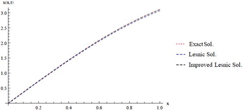
Figure 2. Comparison of the exact, Lesnic and improved Lesnic solutions for ${\vartheta }_5$ at t=1.0.

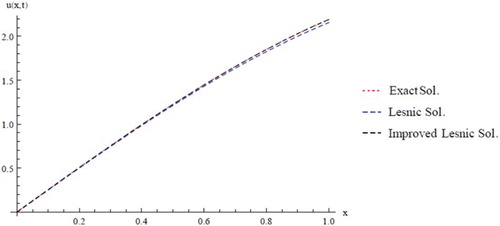
Table 1. Absolute errors of the Improved Lesnic's approach of Example One.

	${\vartheta }_3$	${\vartheta }_5$	${\vartheta }_3$	${\vartheta }_5$
x	t=0.5	t=0.5	t=1.0	t=1.0
0.0	1.37786718e−03	7.20339386e−06	3.03331367e−03	1.15724731e−05
0.1	1.19205842e−03	7.86098384e−06	1.15936032e−03	7.15432778e−05
0.2	8.79086650e−04	7.83740843e−06	9.80275073e−04	1.29831117e−04
0.3	4.60255510e−04	7.22325420e−06	3.32388914e−03	1.85998748e−04
0.4	3.32966490e−05	6.16519070e−06	5.78838161e−03	2.39710735e−04
0.5	5.63705972e−04	4.85058323e−06	8.27636640e−03	2.90714429e−04
0.6	1.08954995e−03	3.48822771e−06	1.06833707e−02	3.38814553e−04
0.7	1.56909026e−03	2.28712552e−06	1.29051501e−02	3.83844405e−04
0.8	1.96360904e−03	1.43535690e−06	1.48451467e−02	4.25636939e−04
0.9	2.24085545e−03	1.08107605e−06	1.64221156e−02	4.63998918e−04
1.0	2.37861775e−03	1.31744824e−06	1.75779431e−02	4.98691029e−04

Example Two: Consider the linear homogeneous wave equation (26) $u_{tt}=u_{xx}-3u,0\le x\le 1,t>0,$(26) with specified conditions (27) $\begin{array}{rl}& u(x,0)=0,u_t(x,0)=2\cos \left(x\right)u_x(0,t)=0,\\ & u_x(1,t)=-\sin \left(1\right)\sin \left(2t\right).\end{array}$(27) With the exact solution (28) $u(x,t)=\cos \left(x\right)\sin \left(2x\right).$(28) Proceeding as above, we obtain the improve Lesnic's approach scheme: (29) $\begin{array}{rl}{u}_0& =\frac{1}{2}(2t\cos (t)-\frac{x^2}{2}\sin (1)\sin (2t)+c(t\left)\right),\\ u_{n+1}& =\frac{1}{2}(L_{tt}^{-1}{L}_{xx}{u}_n+L_{xx}^{-1}{L}_{tt}{u}_n-3L_{xx}^{-1}{u}_n-3L_{tt}^{-1}{u}_n),\\ & n\ge 0.\end{array}$(29) Few terms of Equation (29(29) $\begin{array}{rl}{u}_0& =\frac{1}{2}(2t\cos (t)-\frac{x^2}{2}\sin (1)\sin (2t)+c(t\left)\right),\\ u_{n+1}& =\frac{1}{2}(L_{tt}^{-1}{L}_{xx}{u}_n+L_{xx}^{-1}{L}_{tt}{u}_n-3L_{xx}^{-1}{u}_n-3L_{tt}^{-1}{u}_n),\\ & n\ge 0.\end{array}$(29) ) are $\begin{array}{rl}{u}_0& =\frac{1}{2}(2t\cos (t)-\frac{x^2}{2}\sin (1)\sin (2t)+c(t\left)\right),\\ u_1& =\frac{-2}{3}\cos \left(x\right)t^3+\frac{1}{48}{x}^2(x^2-2)\sin \left(1\right)\sin \left(2t\right),\\ u_2& =\frac{2}{15}\cos \left(x\right)t^5-\frac{1}{1440}{x}^2(x^4-5x^2+7)\\ & \sin \left(1\right)\sin \left(2t\right),\\ & ⋮\end{array}$ Thus, we simulate the scheme in Equation (29(29) $\begin{array}{rl}{u}_0& =\frac{1}{2}(2t\cos (t)-\frac{x^2}{2}\sin (1)\sin (2t)+c(t\left)\right),\\ u_{n+1}& =\frac{1}{2}(L_{tt}^{-1}{L}_{xx}{u}_n+L_{xx}^{-1}{L}_{tt}{u}_n-3L_{xx}^{-1}{u}_n-3L_{tt}^{-1}{u}_n),\\ & n\ge 0.\end{array}$(29) ) and reported the absolutes errors at different times levels in Table 2 and plotted in Figures 3 and 4.

Figure 3. Comparison of the exact, Lesnic and improved Lesnic solutions for ${\vartheta }_5$ at t=0.5.

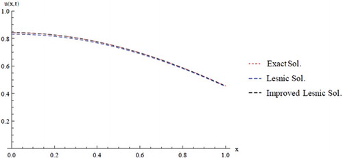
Figure 4. Comparison of the exact, Lesnic and improved Lesnic solutions for ${\vartheta }_5$ at t=1.0.

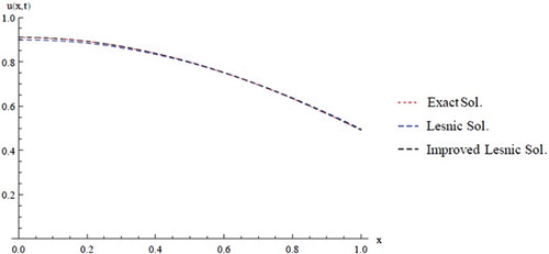
Table 2. Absolute errors of the improved Lesnic's approach of Example Two.

	${\vartheta }_3$	${\vartheta }_5$	${\vartheta }_3$	${\vartheta }_5$
x	t=0.5	t=0.5	t=1.0	t=1.0
0.0	9.78409294e−05	1.24461399e−08	1.20179533e−02	2.50079275e−05
0.1	1.01363262e−04	5.40703719e−08	1.19622480e−02	2.49280386e−05
0.2	1.11556042e−04	1.74873143e−07	1.17953224e−02	2.46852214e−05
0.3	1.27329392e−04	3.63039462e−07	1.15177768e−02	2.42704392e−05
0.4	1.46974006e−04	6.00156261e−07	1.11307074e−02	2.36699706e−05
0.5	1.68314564e−04	8.63002747e−07	1.06358432e−02	2.28672830e−05
0.6	1.88909958e−04	1.12581333e−06	1.00357213e−02	2.18453921e−05
0.7	2.06285951e−04	1.36279561e−06	9.33388646e−03	2.05894746e−05
0.8	2.18182015e−04	1.55065890e−06	8.53509620e−03	1.90894698e−05
0.9	2.22790437e−04	1.67090491e−06	7.64550673e−03	1.73424044e−05
1.0	2.18962307e−04	1.71165272e−06	6.67281480e−03	1.53541940e−05

Example Three: Consider the nonlinear homogeneous equation $u_t+u{u}_x=u_{xx},0\le x\le 1,t>0,$ with specified conditions $u_x(0,t)=\frac{2}{1+2t},u_x(1,t)=\frac{2}{1+2t}.$ The exact solution is given by $u(x,t)=\frac{2}{1+2t}x.$ As in above, we get the improve Lesnic's approach scheme: $\begin{array}{rl}{u}_0& =\frac{2}{1+2t}x,\\ u_{n+1}& =L_{xx}^{-1}{L}_t{u}_n+L_{xx}^{-1}{A}_n,n\ge 0,\end{array}$ where, $A_n$'s are the Adomian polynomials of the nonlinear term $u{u}_x$ expressed using Equation (5(5) $Nu(x,t)=\sum _{n=0}^{\mathrm{\infty }}{A}_n(u_0,u_1,u_2,\dots u_n),$(5) ) with few terms $\begin{array}{rl}{A}_0& =u_0{u}_{0_x},\\ A_1& =u_1{u}_{0_x}+u_0{u}_{1_x},\\ A_2& =u_2{u}_{0_x}+u_1{u}_{1_x}+u_0{u}_{2_x},\\ ⋮\end{array}$ So that, $\begin{array}{rl}{u}_0& =\frac{2}{1+2t}x,\\ u_{n+1}& =0,n\ge 0.\end{array}$ Thus we obtain the exact solution in one iteration without calculating the Adomian polynomials.

4.2. Application of the Improved AADM

Example One: Consider the linear inhomogeneous wave equation (30) $u_{tt}=u_{xx}+2{\pi }^2{\mathrm{e}}^{-\pi t}\sin \left(\pi x\right),0\le x\le 1,t>0,$(30) with specified conditions (31) $\begin{array}{rl}& u(x,0)=\sin \left(\pi x\right),u_t(x,0)=-\pi \sin \left(\pi x\right),u_x(0,t)\\ & =\pi {\mathrm{e}}^{-\pi t},u_x(1,t)=-\pi {\mathrm{e}}^{-\pi t}.\end{array}$(31) With the exact solution (32) $u(x,t)={\mathrm{e}}^{-\pi t}\sin \left(\pi x\right).$(32) As described in the improved AADM procedure, we get the solution of Equations (30(30) $u_{tt}=u_{xx}+2{\pi }^2{\mathrm{e}}^{-\pi t}\sin \left(\pi x\right),0\le x\le 1,t>0,$(30) )–(31(31) $\begin{array}{rl}& u(x,0)=\sin \left(\pi x\right),u_t(x,0)=-\pi \sin \left(\pi x\right),u_x(0,t)\\ & =\pi {\mathrm{e}}^{-\pi t},u_x(1,t)=-\pi {\mathrm{e}}^{-\pi t}.\end{array}$(31) ) given the recursive solution scheme: (33) $\begin{array}{rl}{u}_0& =\frac{1}{2}\left(\right(1-\pi t)\sin (\pi x)\\ & +\pi (x-\mathrm{\Omega }){\mathrm{e}}^{-\pi t}-\frac{\mathrm{\Omega }\pi }{2}{\mathrm{e}}^{-\pi t})\\ & +\frac{1}{2}\left(L_{tt}^{-1}\right(2{\pi }^2{\mathrm{e}}^{-\pi t}\sin \left(\pi x\right))\\ & +L_{xx}^{-1}(2{\pi }^2{\mathrm{e}}^{-\pi t}\sin (\pi x\left)\right)),\\ u_{n+1}& =\frac{1}{2}(-\frac{1}{\mathrm{\Omega }}{\int }_0^{\mathrm{\Omega }}{u}_n(x,t)\mathrm{d}x+L_{tt}^{-1}{L}_{xx}{u}_n+L_{xx}^{-1}{L}_{tt}{u}_n),\\ & n\ge 0.\end{array}$(33) Hence, simulating the scheme in Equation (33(33) $\begin{array}{rl}{u}_0& =\frac{1}{2}\left(\right(1-\pi t)\sin (\pi x)\\ & +\pi (x-\mathrm{\Omega }){\mathrm{e}}^{-\pi t}-\frac{\mathrm{\Omega }\pi }{2}{\mathrm{e}}^{-\pi t})\\ & +\frac{1}{2}\left(L_{tt}^{-1}\right(2{\pi }^2{\mathrm{e}}^{-\pi t}\sin \left(\pi x\right))\\ & +L_{xx}^{-1}(2{\pi }^2{\mathrm{e}}^{-\pi t}\sin (\pi x\left)\right)),\\ u_{n+1}& =\frac{1}{2}(-\frac{1}{\mathrm{\Omega }}{\int }_0^{\mathrm{\Omega }}{u}_n(x,t)\mathrm{d}x+L_{tt}^{-1}{L}_{xx}{u}_n+L_{xx}^{-1}{L}_{tt}{u}_n),\\ & n\ge 0.\end{array}$(33) ); we report the absolutes errors at different times levels in Table 3 and plotted in Figures 5 and 6.

Figure 5. Comparison of the exact, AADM and improved AADM solutions for ${\vartheta }_5$ at t=0.5.

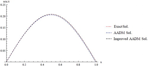
Figure 6. Comparison of the exact, AADM and improved AADM solutions for ${\vartheta }_5$ at t=1.0.

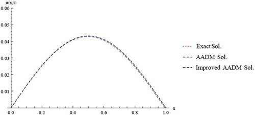
Table 3. Absolute errors of the Improved AADM of Example One.

	${\vartheta }_3$	${\vartheta }_5$	${\vartheta }_3$	${\vartheta }_5$
x	t=0.5	t=0.5	t=1.0	t=1.0
0.0	0.00000000e+00	0.00000000e+00	0.00000000e+00	0.00000000e+00
0.1	1.24404245e−08	1.53119317e−14	2.58611018e−09	3.18303787e−15
0.2	1.58584632e−06	3.12994191e−11	3.29665061e−07	6.50650998e−12
0.3	2.69111041e−05	2.69878974e−09	5.59426892e−06	5.61023268e−10
0.4	1.99690573e−04	6.36178795e−08	4.15115918e−05	1.32248578e−08
0.5	9.40625052e−04	7.36430921e−07	1.95536737e−04	1.53088948e−07
0.6	3.32064156e−03	5.43414960e−06	6.90293560e−04	1.12964872e−06
0.7	9.59955657e−03	2.93779078e−05	1.99555175e−03	6.10706702e−06
0.8	2.39597176e−02	1.26439307e−04	4.98073595e−03	2.62841496e−05
0.9	5.34250805e−02	4.57080210e−04	1.11059831e−02	9.50176405e−05
1.0	1.08938027e−01	1.43962234e−03	2.26459908e−02	2.99268082e−04

Example Two: Consider the nonlinear inhomogeneous wave equation (34) $u_{tt}=u_{xx}+u+u^2-xt-x^2{t}^2,0\le x\le 1,t>0,$(34) with specified conditions (35) $u(x,0)=0,u_t(x,0)=x,u_x(0,t)=t,u_x(1,t)=t.$(35) With the exact solution (36) $u(x,t)=xt.$(36) proceeding as above,the improved AADM recursive solution scheme for Equations (35(35) $u(x,0)=0,u_t(x,0)=x,u_x(0,t)=t,u_x(1,t)=t.$(35) )–(36(36) $u(x,t)=xt.$(36) ) is given by: (37) $\begin{array}{rl}{u}_0& =\frac{1}{2}(xt+(x-\mathrm{\Omega })t+\frac{\mathrm{\Omega }}{2}t-L_{tt}^{-1}(xt+x^2{t}^2)\\ & -L_{xx}^{-1}(xt+x^2{t}^2)),\\ u_{n+1}& =\frac{1}{2}(-\frac{1}{\mathrm{\Omega }}{\int }_0^{\mathrm{\Omega }}{u}_n(x,t)\mathrm{d}x+L_{tt}^{-1}{L}_{xx}{u}_n+L_{xx}^{-1}{L}_{tt}{u}_n)\\ & +\frac{1}{2}(L_{xx}^{-1}{A}_n+L_{tt}^{-1}{A}_n+L_{tt}^{-1}{u}_n+L_{xx}^{-1}{u}_n),\\ & n\ge 0,\end{array}$(37) where, $A_n$'s are the Adomian polynomials of the nonlinear term $u^2$ expressed using Equation (5(5) $Nu(x,t)=\sum _{n=0}^{\mathrm{\infty }}{A}_n(u_0,u_1,u_2,\dots u_n),$(5) ) with few terms $\begin{array}{rl}{A}_0& =u_0^2,\\ A_1& =2u_0{u}_1,\\ A_2& =2u_0{u}_2+u_1^2,\\ A_3& =2u_1{u}_2+2u_0{u}_3,\\ ⋮\end{array}$ Hence, simulating the scheme in Equation (37(37) $\begin{array}{rl}{u}_0& =\frac{1}{2}(xt+(x-\mathrm{\Omega })t+\frac{\mathrm{\Omega }}{2}t-L_{tt}^{-1}(xt+x^2{t}^2)\\ & -L_{xx}^{-1}(xt+x^2{t}^2)),\\ u_{n+1}& =\frac{1}{2}(-\frac{1}{\mathrm{\Omega }}{\int }_0^{\mathrm{\Omega }}{u}_n(x,t)\mathrm{d}x+L_{tt}^{-1}{L}_{xx}{u}_n+L_{xx}^{-1}{L}_{tt}{u}_n)\\ & +\frac{1}{2}(L_{xx}^{-1}{A}_n+L_{tt}^{-1}{A}_n+L_{tt}^{-1}{u}_n+L_{xx}^{-1}{u}_n),\\ & n\ge 0,\end{array}$(37) ); we report the absolutes errors at different times levels in Table 4 and plotted in Figures 7 and 8.

Figure 7. Comparison of the exact, AADM and improved AADM solutions for ${\vartheta }_5$ at t=0.5.

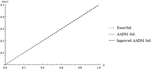
Figure 8. Comparison of the exact, AADM and improved AADM solutions for ${\vartheta }_5$ at t=1.0.

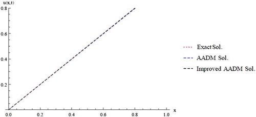
Table 4. Absolute errors of the Improved AADM of Example Two.

	${\vartheta }_3$	${\vartheta }_5$	${\vartheta }_3$	${\vartheta }_5$
x	t=0.5	t=0.5	t=1.0	t=1.0
0.0	0.00000000e+00	0.00000000e+00	0.00000000e+00	0.00000000e+00
0.1	6.43398997e−12	6.91549754e−19	2.46666502e−11	6.52347098e−19
0.2	3.42085723e−10	4.12634542e−15	3.87771135e−09	1.77357486e−15
0.3	2.98009447e−09	6.90350530e−13	8.05986566e−08	1.55634430e−13
0.4	9.29515458e−08	2.68378758e−11	7.28836349e−07	2.90166316e−12
0.5	8.01884656e−07	4.68222023e−10	4.16765332e−06	1.59149835e−11
0.6	4.23898623e−06	4.91551088e−09	1.78086039e−05	6.36894219e−11
0.7	1.67341058e−05	3.63247486e−08	6.21796559e−05	1.46140651e−09
0.8	5.41244863e−05	2.07547868e−07	1.87154966e−04	1.07511806e−08
0.9	1.51265797e−04	9.74287135e−07	5.02763454e−04	4.85612001e−08
1.0	3.77909382e−04	3.91713845e−06	1.23449974e−03	1.39014474e−07

5. Conclusion

In this research, boundary value problems and initial-boundary value problems have been investigated. Improved methods for solving PDEs with Neumann conditions are presented and provided with the recurrence scheme formulae for both the boundary value and initial-boundary value problems. The formulae presented were based on the Lesnic's approach and AADM. Further, these schemes reduced the size of errors at the same time increase the accuracy of the solutions as shown in the given tables; and required less computational work since they do not need to calculate the constants of integration and regard Adomian polynomials meaningless at times. It is also important to mention here that, the propose recursive solution schemes take into account the entire initial and boundary conditions to make possible physically realistic solutions. In future work, further types of problems will be investigated.

Acknowledgments

The authors are grateful to the reviewers for their comments and constructive criticism that significantly contributed in improving the quality of the article.

Disclosure statement

No potential conflict of interest was reported by the authors.

ORCID

H. O. Bakodah  http://orcid.org/0000-0003-1403-5936

N. A. Al-Zaid  http://orcid.org/0000-0003-3612-004X

References

- Wazwaz AM. Partial differential equations and solitary waves theory. Beijing: Higher Education Press; Berlin, Heidelberg: Springer-Verlag; 2009.
- Turkyilmazoglu M. Convergence of the homotopy perturbation method. Int J Nonlinear Sci Numer Simul. 2011;12(1–8):9–14. doi: 10.1515/ijnsns.2011.020
- Liao SJ. Homotopy analysis method: a new analytical technique for nonlinear problems. Commun Nonlinear Sci Numer Simul. 1997;2(2):95–100. doi: 10.1016/S1007-5704(97)90047-2
- He JH. Variational iteration method for autonomous ordinary differential systems. Appl Math Comput. 2000;114(2–3):115–123.
- Adomian G. A review of the decomposition method in applied mathematics. J Math Anal Appl. 1988;135:501–544. doi: 10.1016/0022-247X(88)90170-9
- Bakodah HO. A Comparison study between a Chebyshev collocation method and the Adomian decomposition method for solving linear system of Fredholm integral equations of the second kind. JKAU Sci. 2012;24(1):49–59. doi: 10.4197/Sci.24-1.4
- Wazwaz AM. The modified decomposition method for analytic treatment of differential equations. Appl Math Comput. 2006;173(1):165–176.
- Khan RH, Bakodah HO. Adomian decomposition method and its modification for nonlinear Abel's integral equation. Int J Math Analysis. 2013;7(48):2349–2358. doi: 10.12988/ijma.2013.37179
- Bakodah HO, Darwish MA. Solving Hammerstein type integral equation by new discrete Adomian decomposition methods. Math Probl Eng. 2013;1–5. Article ID 760515.
- Biazar J, Hosseini K. An effective modification of Adomian decomposition method for solving Emden–Fowler type systems. Nat Acad Sci Let. 2017;40(4):285–290. doi: 10.1007/s40009-017-0571-4
- Bakodah HO, Mufti RS, Biswas A. Error estimates of nonlinear algebraic equations by modified Adomain decomposition method. J Comput Theor Nanosc. 2016;13:1–6. doi: 10.1166/jctn.2016.5431
- Nuruddeen RI, Muhammad L, Nass AM, et al. A review of the integral transforms-based decomposition methods and their applications in solving nonlinear PDEs. Palestine J Math. 2018;7:262–280.
- Banaja MA, Al Qarni AA, Bakodah HO, et al. The investigate of optical solitons in cascaded system by improved Adomian decomposition scheme. Optik. 2017;130:1107–1114. doi: 10.1016/j.ijleo.2016.11.125
- Benabidallah M, Cherruault Y. Solving a class of linear partial differential equations with Dirichlet-boundary conditions by the Adomian method. Kybernetes. 2004;33(8):1292–1311. doi: 10.1108/03684920410545270
- Hasni MM, Abdul Majid Z, Senu N. Numerical solution of linear Dirichlet two point boundary value problems using block method. Int J Pure Appl Math. 2013;85(3):495–506. doi: 10.12732/ijpam.v85i3.6
- Gejji VD, Bhalekar S. Solving fractional boundary value problems with Dirichlet boundary conditions using a new iterative method. Comput Math Appl. 2010;59:1801–1809. doi: 10.1016/j.camwa.2009.08.018
- Jiwari R, Pandit S, Mittal RC. A differential quadrature algorithm to solve the two dimensional linear hyperbolic telegraph equation with Dirichlet and Neumann boundary conditions. Appl Math Comput. 2012;218:7279–7294.
- Cheniguel A. Numerical method for the heat equation with Dirichlet and Neumann conditions. Int Multi Conf Eng Comput Sci. 2014;1
- Shibata Y. Neumann problem for one-dimensional nonlinear thermoelasticity Part.. Part Diff Equ Banach Center Publ. 1992;27:457–480. doi: 10.4064/-27-2-457-480
- Dehghan M. Second-order schemes for a boundary value problem with Neumann's boundary conditions. J Comput Appl Math. 2002;138:173–184. doi: 10.1016/S0377-0427(00)00452-0
- Bougoffa L, Al-Mazmumy M. Series solutions to initial-Neumann boundary value problems for parabolic and hyperbolic equations. J Appl Math Inform. 2013;31(1-2):87–97. doi: 10.14317/jami.2013.087
- Kazem S, Rad JA. Radial basis functions method for solving of a non-local boundary value problem with Neumann's boundary conditions. Appl Math Model. 2012;36:2360–2369. doi: 10.1016/j.apm.2011.08.032
- Kaikina EI. Inhomogeneous Neumann initial boundary value problem for the nonlinear Schrodinger equation. J Diff Equ. 2013;255:3338–3356. doi: 10.1016/j.jde.2013.07.036
- Bakodah HO, Al-Zaid NA, Mirzazadeh M, et al. Decomposition method for solving burgers' equation with Dirichlet and Neumann boundary conditions. Optik. 2017;130:1339–1346. doi: 10.1016/j.ijleo.2016.11.140
- Adomian G. A new approach to the heat equation – an application of the decomposition method. J Math Anal Appl. 1986;113:202–209. doi: 10.1016/0022-247X(86)90344-6
- Lesnic D, Elliot L. The decomposition approach to inverse heat conduction. J Math Appl. 1999;232:82–98.
- Aly EH, Ebaid A, Rach R. Advances in the Adomian decomposition method for solving two-point nonlinear boundary value problems with Neumann boundary conditions. Comput Math Appl. 2012;63:1056–1065. doi: 10.1016/j.camwa.2011.12.010
- Lesnic D. A Computational algebraic investigation of the decomposition method for time-dependent problems. Appl Math Comput. 2001;119:197–206.
- Cherruault Y. Convergence of Adomian's method. Kybernotes. 1989;18:31–38. doi: 10.1108/eb005812
- Cherruault Y, Adomian G. Decomposition method: a new proof of convergence. Math Comput Model. 1993;18:103–106. doi: 10.1016/0895-7177(93)90233-O
- Abbaoui K, Cherruault Y. Convergence of Adomian's method applied to nonlinear equations. Math Comput Model. 1994;20:60–73. doi: 10.1016/0895-7177(94)00163-4
- Cherruault Y., Saccomandi G., Some B.. New results for convergence of Adomian's method applied to integral equations. Math Comput Model. 1992;16:85–93. doi: 10.1016/0895-7177(92)90009-A
- Gabet L. The theoretical foundation of the Adomian method. Comput Math Appl. 1994;27:41–52.
- Babolian E, Biazar J. On the order of convergence of Adomian method. Appl Math Comput. 2002;130:383–387.
- Hosseini M, Nasabzadeh H. On the convergence of the Adomian decomposition method. Appl Math Comput. 2006;182:536–543.
- Turkyilmazoglu M. Parametrized Adomian decomposition method with optimum convergence. Trans Model Comput Simul. 2017;27(4). Article No. 21.