Soret–Dufour effects on MHD heat and mass transfer of Walter’s-B viscoelastic fluid over a semi-infinite vertical plate: spectral relaxation analysis

Abstract

Soret–Dufour effects on MHD heat and mass transfer of Walter’s-B viscoelastic fluid over a semi-infinite vertical plate are considered. The equations of motion are set of partial differential equations; these are non-dimensionalized by introducing an appropriate non-dimensional quantity. The dimensionless equations along with the boundary conditions are solved numerically using the spectral relaxation method (SRM). All programs are coded in MATLAB R2012a. Results are presented in graphs, and numerical computations of the local skin friction, local Nusselt number and local Sherwood number are presented in a tabular form. The result revealed that as the viscoelastic parameter increases, the velocity profile close to the plate decreases but when far away from the plate, it increases slightly. The present results were found to be in good agreement with those of the existing literature.

KEYWORDS:

• Soret–Dufour effect
• heat transfer
• viscous dissipation
• thermal radiation
• chemical reaction
• spectral relaxation method

1. Introduction

The physical effects occur in MHD basically when a conductor migrates into a magnetic field, electric current is induced and creates its own magnetic field (Lenz’s law). The conductor used in this paper is the fluid with complex motions. Another important thing to note is that the moment currents are induced probably by a motion of an electrically conducting fluid as a result of a magnetic field; a resistive force acts on the fluid and decelerates its motion. MHD has gained considerable interest due to its fundamental importance in the industrial and technological applications such as in coating of metals, crystal growth, electromagnetic pumps, power generators, MHD accelerators and reactor cooling. Many researchers in the field of fluid dynamics have studied MHD viscoelastic fluid flow by considering the effects of Soret and Dufour number. Soret–Dufour effects have been investigated by numerous scholars in fluid mechanics due to their significance in sciences and engineering like Soret in isotope separation. Gbadeyan et al. [1] considered the effects of Soret and Dufour in their analysis. Their equations of motion were solved using the shooting method with sixth-order of the Runge–Kutta technique. In their analysis, the variation of Dufour in the velocity field is depicted in Figure 1 and it shows that the increase in Dufour number gives a slight increase in the velocity of the fluid. Also, effect of Dufour number as plotted in Figure 10 of their result show that increasing Dufour number increases the fluid temperature. It was discovered in their study that increasing the Soret number increases the concentration boundary layer thickness. They reported that the behaviour of Dufour and Soret on the temperature and concentration profiles is opposite. Choudhury and Kumar Das [2] studied viscoelastic MHD-free convective flow through porous media in the presence of radiation and chemical reaction with heat and mass transfer. Their governing partial differential equations were solved using the multiple perturbation technique. They concluded that the velocity field possesses an accelerating trend with the growing effect of the viscoelastic parameter. Rashidi et al. [3] did not consider the porous medium. The homotopy analysis method with two auxiliary parameters was used and its results show that increasing Soret number or decreasing Dufour number leads to a decrease in velocity and temperature profiles. Vedavathi et al. [4] considered radiation and mass transfer effects on unsteady MHD convective flow over an infinite vertical plate with Dufour and Soret effects. In their analysis, the effects of Soret and Dufour parameters on the velocity, temperature and concentration profiles are plotted in Figures 12(a–c). It is noted that a decrease in Soret number and an increase in Dufour number produce a decrease in the velocity and concentration profiles. In another investigation of Sharma and Aich [5], the effects of Soret and Dufour were significant. They concluded in their study that the rate of flow decreases with an increase in both Soret and Dufour effects. Recently in the work of Hayat et al. [6], the influence of both Soret and Dufour was investigated on the peristaltic flow of Jeffery fluid. The report was made on the study that the behaviour of Soret and Dufour number for temperature and concentration is contradictory. Iqbal and Khalid [7] studied the analysis of thermally developing laminar convection in the finned double-pipe. Ahmed and Iqbal [8] examined MHD power-law fluid flow and heat transfer analysis through Darcy Brinkman porous media in the annular sector. Their results revealed that an increase in the Hartman parameter increases the rate of heat transfer. Ahmed et al. [9] examined the study of forced convective power-law fluid through an annulus sector duct numerically. Numerical study of heat transfer and fluid flow through an annular sector duct filled with porous media was carried out by Iqbal and Afag Hamna [10]. Iqbal et al. [11] recently considered the simulation of MHD-forced convection heat transfer through the annular sector.

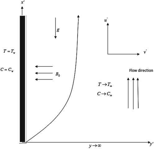
Figure 1: Physical model of the problem.

The role of the magnetic field and surface corrugation on natural convection in a nanofluid-filled 3D trapezoidal cavity was carried out by Selimefendigil and Oztop [12]. Conjugate natural convection in a nanofluid-filled partitioned horizontal annulus formed by two isothermal cylinder surfaces under magnetic field was investigated by Selimefendigil and Oztop [13]. The work of Selimefendigil et al. [14] deals with the flow of MHD in a lid-driven nanofluid-filled square cavity with a flexible side wall. Finite element formulation was used as a method of solution and their findings revealed that the Brownian motion effect on the thermal conductivity of the nanofluid is significant. The finite element method was used to solve the analysis of MHD mixed convection in a flexible-walled and nanofluid- filled the lid-driven cavity with volumetric heat generation by Selimefendigil and Oztop [15]. The study revealed that decreasing values of Richardson number and increasing values of Hartmann number decreases the average heat transfer.

Non-Newtonian fluids are important in many technological applications compared to the Newtonian fluids. The non-Newtonian fluid flows find applications in modern technology and in industries. The non-linearity of the mechanism of non-Newtonian fluids presents a challenge to mathematicians, engineers and physicists. This non-linearity manifests itself in fields such as food, drilling operations and bioengineering. Rashidi et al. [16] examined analytic approximate solutions for MHD boundary-layer viscoelastic fluid flow over a continuously moving stretching surface by the homotopy analysis method with two auxiliary parameters. Graphical results of Figures 7 and 8 show that the velocity decreases with increasing viscoelastic parameter. Sivaraj and Kumar [17] examined chemically reacting dusty viscoelastic fluid flow in an irregular channel with convective boundary. They reported that velocity profiles of all physical parameters decrease at the wavy wall. Manglesh and Gorla [18] studied the effects of thermal radiation, chemical reaction and rotation on unsteady MHD viscoelastic slip flow. They reported in their study that increasing the viscoelastic parameter makes the hydrodynamic boundary layer to adhere strongly to the surface and results in the retardation of the flow to the left half channel but accelerates in the right half when there is no slip boundary condition. In 2013, Kumar and Sivaraj [19] examined heat and mass transfer in MHD viscoelastic fluid flow over a vertical cone and flat plate with variable viscosity. They reported in the study that magnetic field, buoyancy ratio parameter, viscosity variation parameter, Eckert number and chemical reaction parameter play an important role in viscoelastic fluid flow through the porous medium. In the work of Eswaramoorthi et al. [20], viscoelastic type of fluid was considered. The flow equations were solved using the homotopy analysis method. It was reported in the study that increasing the viscoelastic parameter results in a decrease in the velocity. Graphical result of Figure 10 shows that increasing the viscoelastic parameter leads to a decrease in the temperature.Finite element analysis of MHD viscoelastic nanofluid flow over a stretching sheet with radiation is examined by Madhu and Kishan [21].

In 2013, Rao et al. [22] studied finite element analysis of radiation and mass transfer flow pass over a semi-infinite moving vertical plate with viscous dissipation. In their study, they neglected the effects of Soret and Dufour parameters. In 2016, Alao et al. [23] considered the effects of thermal radiation, Soret and Dufour on an unsteady heat and mass transfer flow of a chemically reacting fluid pass over a semi-infinite vertical plate with viscous dissipation. The work of Alao et al. [23] was an extension of Rao et al’s. [22] work by considering the effects of Soret and Dufour parameters in their governing equations. The two problems are centred on Newtonian fluid.

The present study is a Non-Newtonian fluid model. Its objective is to illustrate the use of the spectral relaxation method (SRM) for solving the equations of motion representing the physical model of Soret–Dufour effects on MHD heat and mass transfer of Walter’s B viscoelastic fluid over a semi-infinite vertical plate and to explore the effects of different controlling flow parameters as encountered in the equations. SRM is an iterative method that employs the Gauss–Seidel approach in solving both linear and non-linear different equations. SRM is found to be effective and accurate. The governing equations are systems of partial differential equations which are transformed into a dimensionless form by introducing suitable non-dimensional quantities. Numerical computations are carried out and graphical results for the velocity, temperature, and concentration profiles as well as the local skin friction, local Nusselt number and local Sherwood number coefficients within the boundary layer flow are discussed.

2. Equations of motion

The unsteady free convective flow of a viscoelastic fluid (Walters B’ model) over a semi-infinite vertical plate with time-dependent oscillatory suction in the presence of a transfer magnetic field is considered. The plate is considered infinite in the $x^{\mathrm{\prime }}$-direction, thus the $x^{\mathrm{\prime }}$-axis shall be taken along the vertical infinite plate in the upward direction and the $y^{\mathrm{\prime }}$-axis normal to the plate (see Figure 1). The flow direction is vertically upward and in the continuity equation, the term $\mathrm{\partial }{u}^{\mathrm{\prime }}/\mathrm{\partial }{x}^{\mathrm{\prime }}$ is neglected. It is assumed that initially at $t^{\mathrm{\prime }}\le 0$, the plate and fluid are at the same temperature. Soret, Dufour, heat generation or absorption is taken into account. It is assumed that the magnetic Reynolds number is small so that the induced magnetic field is neglected. In the direction of the$y^{\mathrm{\prime }}$-axis, a magnetic field of uniform strength $B_0$ is applied. Walters-B viscoelastic type of fluid is considered in this paper.

Following Choudhury and Kumar Das [2], the constitutive equation for Walter’s-B viscoelastic fluid can be defined as (1) ${\sigma }_{ik}=-p{g}_{ik}+{\sigma }_{ik}^{\mathrm{\prime }}$(1) (2) ${\sigma }^{\mathrm{\prime }ik}=a{\eta }_0{e}^{ik}-2k_{0}e{}^{\mathrm{\prime }ik}$(2) where ${\eta }_0$ is the limiting viscosity at small rates of shear, $k_0$ is the elastic co-efficient, ${\sigma }^{ik}$ is the stress tensor, $p$ is the isotropic pressure, $g_{ik}$ is the metric tensor of a fixed co-ordinate system $x^i$ and $v_i$ is the velocity vector. The contravariant form of $e^{\mathrm{\prime }ik}$ is given as (3) $e^{\mathrm{\prime }ik}=\frac{\mathrm{\partial }{e}^{ik}}{\mathrm{\partial }t}+v^m{e}_{,m}^{ik}-V_{,m}^k{e}^{im}-v_{,m}^i{e}^{mk}$(3)

The convected derivative of the deformation rate tensor $e^{ik}$ is defined by (4) $2e^{ik}=v_{i,k}+v_{k,i}$(4)

Here, ${\eta }_0$ is the limiting viscosity at the small rate of shear and is given as (5) ${\eta }_0={\int }_0^{\mathrm{\infty }}N\left(\tau \right)d\tau \text{and }{k}_0={\int }_0^{\mathrm{\infty }}\tau N\left(\tau \right)d\tau$(5) $N\left(\tau \right)$ is the relaxation spectrum as discussed by Walters [24]. This idealized model is a valid approximation of Walters-B taking short relaxation time into account so that terms involving (6) ${\int }_0^{\mathrm{\infty }}{t}^{n}N\left(\tau \right)d\tau ,n\ge 2$(6) have been neglected in the momentum equation and $k_0$ is significant.

Under the above assumptions and the usual Boussinesq’s approximation, the governing equations and boundary conditions are given as (see details in Alao et al. [23]) (7) $\frac{\mathrm{\partial }{v}^{\mathrm{\prime }}}{\mathrm{\partial }{y}^{\mathrm{\prime }}}=0$(7) (8) $\begin{array}{rl}& \frac{\mathrm{\partial }{u}^{\mathrm{\prime }}}{\mathrm{\partial }{t}^{\mathrm{\prime }}}+v^{\mathrm{\prime }}\frac{\mathrm{\partial }{u}^{\mathrm{\prime }}}{\mathrm{\partial }{y}^{\mathrm{\prime }}}=\nu \frac{{\mathrm{\partial }}^2{u}^{\mathrm{\prime }}}{\mathrm{\partial }{y^{\mathrm{\prime }}}^2}+g{\beta }_t\left(T-T_{\mathrm{\infty }}\right)+g{\beta }_c\left(C-C_{\mathrm{\infty }}\right)\\ & -\frac{\sigma B_0^{2}u}{\rho }-\frac{K_0}{\rho }\left(\frac{{\mathrm{\partial }}^3{u}^{\mathrm{\prime }}}{\mathrm{\partial }{t}^{\mathrm{\prime }}\mathrm{\partial }y{}^{\mathrm{\prime }2}}+v^{\mathrm{\prime }}\frac{{\mathrm{\partial }}^3{u}^{\mathrm{\prime }}}{\mathrm{\partial }y{}^{\mathrm{\prime }3}}\right)\end{array}$(8) (9) $\begin{array}{rl}& \frac{\mathrm{\partial }T}{\mathrm{\partial }{t}^{\mathrm{\prime }}}+v^{{}^{\mathrm{\prime }}\frac{\mathrm{\partial }T}{\mathrm{\partial }{y}^{\mathrm{\prime }}}}=\alpha \frac{{\mathrm{\partial }}^{2}T}{\mathrm{\partial }{y^{\mathrm{\prime }}}^2}-\frac{1}{\rho c_p}\frac{\mathrm{\partial }{q}_r}{\mathrm{\partial }{y}^{\mathrm{\prime }}}+\frac{\mu }{\rho c_p}{\left(\frac{\mathrm{\partial }{u}^{\mathrm{\prime }}}{\mathrm{\partial }{y}^{\mathrm{\prime }}}\right)}^2\\ & +\frac{D{K}_T{\mathrm{\partial }}^{2}C}{C_s{c}_p\mathrm{\partial }{y^{\mathrm{\prime }}}^2}+\frac{{\beta }^{\ast }u}{\rho c_p}\left(T_{\mathrm{\infty }}-T\right)+\frac{Q_0}{\rho c_p}\left(T-T_{\mathrm{\infty }}\right)\end{array}$(9) (10) $\frac{\mathrm{\partial }C}{\mathrm{\partial }{t}^{\mathrm{\prime }}}+v^{\mathrm{\prime }}\frac{\mathrm{\partial }C}{\mathrm{\partial }{y}^{\mathrm{\prime }}}=D\frac{{\mathrm{\partial }}^{2}C}{\mathrm{\partial }y{}^{\mathrm{\prime }2}}-K_{r^{\mathrm{\prime }}}^2\left(C-C_{\mathrm{\infty }}\right)+\frac{D{K}_T{\mathrm{\partial }}^{2}T}{T_m\mathrm{\partial }y{}^{\mathrm{\prime }2}}$(10) subject to the conditions (11) $\begin{array}{rl}u& =U_0,T=T_w+\psi \left(T_w-T_{\mathrm{\infty }}\right)e^{n^{\mathrm{\prime }}{t}^{\mathrm{\prime }}},\\ C& =C_w+\psi \left(C_w-C_{\mathrm{\infty }}\right)e^{n^{\mathrm{\prime }}{t}^{\mathrm{\prime }}}at{y}^{\mathrm{\prime }}=0\end{array}$(11) (12) $u\to 0,T\to T_{\mathrm{\infty }},C\to C_{\mathrm{\infty }}\text{ as }{y}^{\mathrm{\prime }}\to \mathrm{\infty }$(12) ${\beta }^{\ast }\left(T_{\mathrm{\infty }}-T\right)$ and $Q_0\left(T-T_{\mathrm{\infty }}\right)$ are the heat generation and absorption, respectively.

Both sides of the continuity equation (7) are integrated to get $v^{\mathrm{\prime }}=\text{constant}$. Obviously, the suction velocity normal to the plate is a constant function or assumed as a function of time. In this paper, it is considered as a case when it is both constant and time-dependent expressed as [23] (13) $v^{\mathrm{\prime }}=-v_0\left(1+\epsilon A{e}^{n^{\mathrm{\prime }}{t}^{\mathrm{\prime }}}\right)$(13)

It is assumed in this paper that $\mathrm{\partial }{q}_r/\mathrm{\partial }{y}^{\mathrm{\prime }}>>\mathrm{\partial }{q}_r/\mathrm{\partial }{x}^{\mathrm{\prime }}$ and as a result the $x^{\mathrm{\prime }}$-direction radiative flux $\mathrm{\partial }{q}_r/\mathrm{\partial }{x}^{\mathrm{\prime }}$ is neglected. However, the radiative heat flux that dominates the flow is $\mathrm{\partial }{q}_r/\mathrm{\partial }{y}^{\mathrm{\prime }}$.

Assuming that the temperature difference within the flow regime is sufficiently small in such a way that $T^4$ can be expressed as a linear function of the free stream temperature $T_{\mathrm{\infty }}$. Expanding $T^4$ in the Taylor series about $T_{\mathrm{\infty }}$ and neglecting the higher terms let us consider the Taylor series expansion of the function $m\left(x\right)$ about $x_0$ (14) $\begin{array}{rl}m\left(x\right)& =m\left(x_0\right)+\left(x-x_0\right)m^{\mathrm{\prime }}\left(x_0\right)+\frac{{(x-x_0)}^2}{2!}{m}^{\mathrm{\prime \prime }}\left(x_0\right)\\ & +\cdots +\frac{{(x-x_0)}^n}{n!}{m}^n\left(x_0\right)\end{array}$(14) setting $m\left(x\right)=T^4$ and $m\left(x_0\right)=m\left(T_{\mathrm{\infty }}\right)=T_{\mathrm{\infty }}^4$ in the equation above and neglecting higher order term lead to: (15) $T^4=4T_{\mathrm{\infty }}^{3}T-3T_{\mathrm{\infty }}^4$(15)

Using the Roseland approximation, the radiative heat flux is given by (16) $q_r=-\frac{4{\sigma }_e}{3k_e}\frac{\mathrm{\partial }{T}^4}{\mathrm{\partial }{y}^{\mathrm{\prime }}}$(16) where ${\sigma }_e$ is the Stefan–Boltzmann constant and $k_e$ is the mean absorption coefficient. By using the Roseland approximation, the present study is limited to optically thick fluids. If temperature differences within the flow are sufficiently small, then Equation (15) can be linearized and in view of Equations (15) and (16), Equation (9) reduces to (17) $\begin{array}{rl}& \frac{\mathrm{\partial }T}{\mathrm{\partial }{t}^{\mathrm{\prime }}}+v^{\mathrm{\prime }}\frac{\mathrm{\partial }T}{\mathrm{\partial }y}=\alpha \frac{{\mathrm{\partial }}^{2}T}{\mathrm{\partial }y{}^{\mathrm{\prime }2}}+\frac{16{\sigma }_e}{3\rho c_p{k}_e}{T}_{\mathrm{\infty }}^3\frac{{\mathrm{\partial }}^{2}T}{\mathrm{\partial }y{}^{\mathrm{\prime }2}}+\frac{\mu }{\rho c_p}(\frac{\mathrm{\partial }{u}^{\mathrm{\prime }}}{\mathrm{\partial }{y}^{\mathrm{\prime }}}{)}^2\\ & +\frac{D_m}{C_s}\frac{k_T}{c_p}\frac{{\mathrm{\partial }}^{2}C}{\mathrm{\partial }y{}^{\mathrm{\prime }2}}+\frac{{\beta }^{\ast }u}{\rho c_p}\left(T_{\mathrm{\infty }}-T\right)+\frac{Q_0}{\rho c_p}\left(T-T_{\mathrm{\infty }}\right)\end{array}$(17)

In order to write the governing equations and the boundary conditions in dimensionless form, the following non-dimensional quantities are introduced: (18) $u=\frac{u^{\mathrm{\prime }}}{u_0},y=\frac{v_0^2{y}^{\mathrm{\prime }}}{\upsilon },t=\frac{v_0^2{t}^{\mathrm{\prime }}}{\upsilon },n=\frac{\upsilon n^{\mathrm{\prime }}}{v_0^2}$(18) (19) $\vartheta =\frac{T-T_{\mathrm{\infty }}}{T_w-T_{\mathrm{\infty }}},\varphi =\frac{C-C_{\mathrm{\infty }}}{C_w-C_{\mathrm{\infty }}},P_r=\frac{\upsilon \rho c_p}{k}=\frac{\upsilon }{\alpha }$(19) (20) $S_c=\frac{\upsilon }{D},G_r=\frac{g\beta v\left(T_w-T_{\mathrm{\infty }}\right)}{u_0{v}_0^2},G_m=\frac{g{\beta }^{\ast }v\left(C_w-C_{\mathrm{\infty }}\right)}{u_0{v}_0^2}$(20) (21) $E_c=\frac{u_0^2}{c_p\left(T_w-T_{\mathrm{\infty }}\right)},\alpha =\frac{K_0{V}_0^2}{\rho {\nu }^2},\mathrm{\Delta }=\frac{{\beta }^{\ast }{u}_0\nu }{\rho c_p{v}_0^2}$(21) (22) $k_r^2=\frac{k_r{}^{\mathrm{\prime }2}v}{v_0^2},Rr=\frac{16{\sigma }_e{T}_{\mathrm{\infty }}^3}{3k_{e}k},M=\frac{\sigma B_0^{2}v}{\rho v_0^2},{\delta }_x=\frac{Q_0\nu }{\rho c_p{v}_0^2}$(22)

The above non-dimensional quantities on the governing momentum, energy, concentration equations and the boundary conditions lead to (23) $\begin{array}{rl}& \frac{\mathrm{\partial }u}{\mathrm{\partial }t}-\left(1+\epsilon A{e}^{nt}\right)\frac{\mathrm{\partial }u}{\mathrm{\partial }y}=\frac{{\mathrm{\partial }}^{2}u}{\mathrm{\partial }{y}^2}+G_r\vartheta +G_m\varphi -M^{2}u\\ & -\alpha \left(\frac{{\mathrm{\partial }}^{3}u}{\mathrm{\partial }t\mathrm{\partial }{y}^2}-\left(1+\epsilon e^{nt}\right)\frac{{\mathrm{\partial }}^{3}u}{\mathrm{\partial }{y}^3}\right)\end{array}$(23) (24) $\begin{array}{rl}& \frac{\mathrm{\partial }\vartheta }{\mathrm{\partial }t}-\left(1+\epsilon A{e}^{nt}\right)\frac{\mathrm{\partial }\vartheta }{\mathrm{\partial }y}=\left(\frac{1+Rr}{P_r}\right)\frac{{\mathrm{\partial }}^2\vartheta }{\mathrm{\partial }{y}^2}+E_c{\left(\frac{\mathrm{\partial }u}{\mathrm{\partial }y}\right)}^2\\ & +D_u\frac{{\mathrm{\partial }}^2\varphi }{\mathrm{\partial }{y}^2}+{\delta }_x\vartheta -\mathrm{\Delta }u\vartheta \end{array}$(24) (25) $\frac{\mathrm{\partial }\varphi }{\mathrm{\partial }t}-\left(1+\epsilon A{e}^{nt}\right)\frac{\mathrm{\partial }\varphi }{\mathrm{\partial }y}=\frac{1}{S_c}\frac{{\mathrm{\partial }}^2\varphi }{\mathrm{\partial }{y}^2}-k_r^2\varphi +S_r\frac{{\mathrm{\partial }}^2\vartheta }{\mathrm{\partial }{y}^2}$(25) where $G_r$, $G_m$, $P_r$, $Rr$, $E_c$, $S_c$, $k_r$, $D_u$ ,$S_r$, $\alpha$, $\mathrm{\Delta }$ and ${\delta }_x$ are the thermal Grashof number, mass Grashof number, Prandtl number, radiation parameter, Eckert number, Schmidt number, chemical reaction parameter, Dufour number, Soret number, viscoelastic parameter, heat generation/absorption coefficient and heat source/sink parameter, respectively.

The transformed initial and boundary conditions are (26) $\epsilon e^{nt}\text{ at }y=0$(26) (27) $u\to 0,\vartheta \to 0,\varphi \to 0,\text{ at }y\to \mathrm{\infty }$(27)

The physical quantities of interest are the local skin friction coefficient $\left(Cf\right)$, local Nusselt number $\left(Nu\right)$ and Sherwood number $\left(Sh\right)$ of the flow in practical engineering. The skin friction coefficient, Nusselt and Sherwood number are given as $Cf=\frac{{\tau }_w}{\rho U_0{V}_0},Nu=-\frac{K{q}_w}{T_w-T_{\mathrm{\infty }}},Sh=\frac{D{\left(\frac{\mathrm{\partial }C}{\mathrm{\partial }{y}^{\mathrm{\prime }}}\right)}_{y^{\mathrm{\prime }}=0}}{C_w-C_{\mathrm{\infty }}}$ where ${\tau }_w={\eta }_0\frac{\mathrm{\partial }u}{\mathrm{\partial }{y}^{\mathrm{\prime }}}\left|{}_{y=0}-K_0{\left[\frac{{\mathrm{\partial }}^2{u}^{\mathrm{\prime }}}{\mathrm{\partial }{t}^{\mathrm{\prime }}\mathrm{\partial }{y}^{\mathrm{\prime }}}+\frac{{\mathrm{\partial }}^2{u}^{\mathrm{\prime }}}{\mathrm{\partial }{y}^{{}^{\mathrm{\prime }}2}}\right]}_{y=0}\right.$ $q_w=-K{\left(\frac{\mathrm{\partial }C}{\mathrm{\partial }{y}^{\mathrm{\prime }}}\right)}_{y=0}-\frac{4{\sigma }_e}{3k_e}{\left(\frac{\mathrm{\partial }{T}^4}{\mathrm{\partial }{y}^{\mathrm{\prime }}}\right)}_{y=0}.$

3. Method of solution

The non-dimensionless transformed system of partial differential equations is solved in this section using the spectral relaxation method (SRM). SRM is an iterative procedure that employs the Gauss–Siedel type of relaxation approach to linearize and decouple the system of coupled differential equations. The resulting non-linear differential equations are further discretized and solved with the Chebyshev pseudo-spectral method [25]. The linear terms in each equation are evaluated at the current iteration level (denoted by $r+1$) and the non-linear terms are assumed to be known from the previous iteration level (denoted by $r$). The following are the basic steps of the method:

1. decoupling and rearrangement of the governing non-linear equations in a Gauss–Siedel manner.

2. discretizing the linear differential equations.

3. solving the discretized linear differential equations iteratively using the Chebyshev pseudo-spectral method.

Applying the spectral relaxation method (SRM), we first re-arrange the transformed governing Equations (23)–(25) to yield; (28) $\begin{array}{rl}\frac{\mathrm{\partial }u}{\mathrm{\partial }t}+\alpha \frac{{\mathrm{\partial }}^{3}u}{\mathrm{\partial }t\mathrm{\partial }{y}^2}& =\left(1+\epsilon A{e}^{nt}\right)\frac{\mathrm{\partial }u}{\mathrm{\partial }y}+\frac{{\mathrm{\partial }}^{2}u}{\mathrm{\partial }{y}^2}+G_r\vartheta \\ & +G_m\varphi -M^{2}u-\alpha \left(1+\epsilon e^{nt}\right)\frac{{\mathrm{\partial }}^{3}u}{\mathrm{\partial }{y}^3}\end{array}$(28) (29) $\begin{array}{rl}\frac{\mathrm{\partial }\vartheta }{\mathrm{\partial }t}& =\left(1+\epsilon A{e}^{nt}\right)\frac{\mathrm{\partial }\vartheta }{\mathrm{\partial }y}+\left(\frac{1+Rr}{P_r}\right)\frac{{\mathrm{\partial }}^2\vartheta }{\mathrm{\partial }{y}^2}+E_c{\left(\frac{\mathrm{\partial }u}{\mathrm{\partial }y}\right)}^2\\ & +D_u\frac{{\mathrm{\partial }}^2\varphi }{\mathrm{\partial }{y}^2}+{\delta }_x\vartheta -\mathrm{\Delta }u\vartheta \end{array}$(29) (30) $\frac{\mathrm{\partial }\varphi }{\mathrm{\partial }t}=\left(1+\epsilon A{e}^{nt}\right)\frac{\mathrm{\partial }\varphi }{\mathrm{\partial }y}+\frac{1}{S_c}\frac{{\mathrm{\partial }}^2\varphi }{\mathrm{\partial }{y}^2}-k_r^2\varphi +S_r\frac{{\mathrm{\partial }}^2\vartheta }{\mathrm{\partial }{y}^2}$(30)

subject to (31) $u=1,\vartheta =1+\epsilon e^{nt},\varphi =1+\epsilon e^{nt}\text{ at }y=0$(31) (32) $u\to 0,\vartheta \to 0,\varphi \to 0,\text{ at }y\to \mathrm{\infty }$(32)

Adopting the SRM on the non-linear coupled partial differential equations (28)–(30) subject to (31) and (32), to obtain (33) $\begin{array}{rl}\frac{\mathrm{\partial }{u}_{r+1}}{\mathrm{\partial }t}+\alpha \frac{{\mathrm{\partial }}^2{u}_{r+1}}{\mathrm{\partial }{t}^2}& =\beta \frac{{\mathrm{\partial }}^3{u}_{r+1}}{\mathrm{\partial }{y}^3}+\frac{{\mathrm{\partial }}^2{u}_{r+1}}{\mathrm{\partial }{y}^2}+\beta \frac{\mathrm{\partial }{u}_{r+1}}{\mathrm{\partial }y}\\ & +Gr{\vartheta }_r+Gm{\varphi }_r-M^2{u}_{r+1}\end{array}$(33) (34) $\begin{array}{rl}Pr\frac{\mathrm{\partial }{\vartheta }_{r+1}}{\mathrm{\partial }t}& =\left(1+Rr\right)\frac{{\mathrm{\partial }}^2{\vartheta }_{r+1}}{\mathrm{\partial }{y}^2}+PrEc{\left(\frac{\mathrm{\partial }{u}_{r+1}}{\mathrm{\partial }y}\right)}^2+PrDu\frac{{\mathrm{\partial }}^2{\varphi }_r}{\mathrm{\partial }{y}^2}\\ & +Pr{\delta }_x{\vartheta }_{r+1}+Pr\mathrm{\Delta }{u}_r{\vartheta }_{r+1}+Pr\beta \frac{\mathrm{\partial }{\vartheta }_{r+1}}{\mathrm{\partial }y}\end{array}$(34) (35) $\begin{array}{rl}Sc\frac{\mathrm{\partial }{\varphi }_{r+1}}{\mathrm{\partial }t}& =\frac{{\mathrm{\partial }}^2{\varphi }_{r+1}}{\mathrm{\partial }{y}^2}+Sc\beta \frac{\mathrm{\partial }{\varphi }_{r+1}}{\mathrm{\partial }y}-Sc{k}_r^2{\varphi }_{r+1}\\ & +ScSr\frac{{\mathrm{\partial }}^2{\vartheta }_{r+1}}{\mathrm{\partial }{y}^2}\end{array}$(35) subject to (36) $\begin{array}{rl}{u}_{r+1}\left(0,t\right)& =1,{\vartheta }_{r+1}\left(0,t\right)=1+\epsilon e^{nt},\\ {\varphi }_{r+1}\left(0,t\right)& =1+\epsilon e^{nt}\end{array}$(36) (37) $u_{r+1}\left(\mathrm{\infty },t\right)=0,{\vartheta }_{r+1}\left(\mathrm{\infty },t\right)=0,{\varphi }_{r+1}\left(\mathrm{\infty },t\right)=0$(37) where $\beta =1+\epsilon A{e}^{nt}$, setting (38) $\begin{array}{rl}{a}_{0,r}& =\beta =1+\epsilon A{e}^{nt},a_{1,r}=\beta =1+\epsilon A{e}^{nt},\\ a_{2,r}& =Gr{\vartheta }_r+Gm{\varphi }_r,b_{0,r}=(1+Rr),\\ b_{1,r}& =Pr\beta =Pr\left(1+\epsilon A{e}^{nt}\right),b_{2,r}=PrEc{\left(\frac{\mathrm{\partial }{u}_{r+1}}{\mathrm{\partial }\text{y}}\right)}^2,\\ b_{3,r}& =PrDu\frac{{\mathrm{\partial }}^2{\varphi }_r}{\mathrm{\partial }{y}^2},b_{4,r}=Pr\mathrm{\Delta }{u}_r,\\ c_{0,r}& =Sc\beta =Sc\left(1+\epsilon A{e}^{nt}\right),c_{1,r}=ScSr\frac{{\mathrm{\partial }}^2{\vartheta }_{r+1}}{\mathrm{\partial }{y}^2}\end{array}$(38)

Substituting the above coefficient parameters into (33)–(35) gives (39) $\begin{array}{rl}\frac{\mathrm{\partial }{u}_{r+1}}{\mathrm{\partial }t}+\alpha \frac{{\mathrm{\partial }}^3{u}_{r+1}}{\mathrm{\partial }t\mathrm{\partial }{y}^2}& =a_{1,r}\frac{\mathrm{\partial }{u}_{r+1}}{\mathrm{\partial }y}+\frac{{\mathrm{\partial }}^2{u}_{r+1}}{\mathrm{\partial }{y}^2}+a_{2,r}\\ & -M^2{u}_{r+1}+a_{0,r}\frac{{\mathrm{\partial }}^3{u}_{r+1}}{\mathrm{\partial }{y}^3}\end{array}$(39) (40) $\begin{array}{rl}\frac{\mathrm{\partial }{\vartheta }_{r+1}}{\mathrm{\partial }t}& =b_{1,r}\frac{\mathrm{\partial }{\vartheta }_{r+1}}{\mathrm{\partial }y}+b_{0,r}\frac{{\mathrm{\partial }}^2{\vartheta }_{r+1}}{\mathrm{\partial }{y}^2}+b_{2,r}+b_{3,r}\\ & +Pr{\delta }_x{\vartheta }_{r+1}-b_{4,r}{\vartheta }_{r+1}\end{array}$(40) (41) $\frac{\mathrm{\partial }{\varphi }_{r+1}}{\mathrm{\partial }t}=c_{0,r}\frac{\mathrm{\partial }{\varphi }_{r+1}}{\mathrm{\partial }y}+\frac{{\mathrm{\partial }}^2{\varphi }_{r+1}}{\mathrm{\partial }{y}^2}-k_r^2{\varphi }_{r+1}+c_{1,r}$(41) subject to (42) $\begin{array}{rl}{u}_{r+1}\left(0,t\right)& =1,{\vartheta }_{r+1}\left(0,t\right)=1+\epsilon e^{nt},\\ {\varphi }_{r+1}\left(0,t\right)& =1+\epsilon e^{nt}\text{ at }y=0\end{array}$(42) (43) $\begin{array}{rl}{u}_{r+1}\left(\mathrm{\infty },t\right)& =0,{\vartheta }_{r+1}\left(\mathrm{\infty },t\right)=0,\\ {\varphi }_{r+1}\left(\mathrm{\infty },t\right)& =0,\text{ at }y\to \mathrm{\infty }\end{array}$(43)

The unknown functions are defined by the Gauss–Lobatto points given as (44) ${\xi }_j=\text{cos}\frac{\pi j}{N},j=0,1,2,\dots ,N;1\le \xi \le -1$(44) where $N$ is the number of collocation points. The domain of the physical region $\left[0,\mathrm{\infty }\right)$ is transformed into $\left[-1,1\right]$. Thus, the problem is solved on the interval $\left[0,L\right]$ instead of $\left[0,\mathrm{\infty }\right)$. The following transformation is used to map the interval together (45) $\frac{\eta }{L}=\frac{\xi +1}{2},-1\le \xi \le 1$(45) where L is the scaling parameter used to implement the boundary conditions at infinity. The initial approximations for solving Equations (23)–(25) are obtained at $y=0$ and are chosen with due consideration of the boundary conditions (26) and (27). Hence, $u_0\left(y,t\right),{\vartheta }_0\left(y,t\right)$ and ${\varphi }_0\left(y,t\right)$ are chosen as follows: (46) $u_0\left(y,t\right)=e^{-y},{\vartheta }_0\left(y,t\right)={\varphi }_0\left(y,t\right)=e^{-y}+\epsilon e^{nt}$(46)

The system of Equations (39)–(41) can be solved iteratively for the unknown functions starting from the initial approximations in (46). The iteration schemes (39), (40) and (41) are solved iteratively for $u_{r+1}\left(y,t\right),{\vartheta }_{r+1}\left(y,t\right)$ and ${\varphi }_{r+1}\left(y,t\right)$ when $r=0,1,2$. In order to solve the system of Equations (39)–(41), the equations are discretized with the help of the Chebyshev spectral collocation method in the $y-$direction and the implicit finite difference method in the $t-$direction. The finite difference scheme is used with centring about a mid-point between $t^{n+1}$ and $t^n$. The mid-point is expressed as (47) $t^{n+\frac{1}{2}}=\frac{t^{n+1}+t^n}{2}$(47)

Thus using the centring about $t^{n+\frac{1}{2}}$ to the unknown functions, say $u\left(y,t\right),\vartheta \left(y,t\right)$ and $\varphi \left(y,t\right)$ and its associated derivative yield (48) $\begin{array}{rl}u\left(y_j,t^{n+\frac{1}{2}}\right)& =u_j^{n+\frac{1}{2}}=\frac{u_j^{n+1}+u_j^n}{2},\\ {\left(\frac{\mathrm{\partial }u}{\mathrm{\partial }t}\right)}^{n+\frac{1}{2}}& =\frac{u_j^{n+1}-u_j^n}{\mathrm{\Delta }t}\end{array}$(48) (49) $\begin{array}{rl}\vartheta \left(y_j,t^{n+\frac{1}{2}}\right)& ={\vartheta }_j^{n+\frac{1}{2}}=\frac{{\vartheta }_j^{n+1}+{\vartheta }_j^n}{2},\\ {\left(\frac{\mathrm{\partial }\vartheta }{\mathrm{\partial }t}\right)}^{n+\frac{1}{2}}& =\frac{{\vartheta }_j^{n+1}-{\vartheta }_j^n}{\mathrm{\Delta }t}\end{array}$(49) (50) $\begin{array}{rl}\varphi \left(y_j,t^{n+\frac{1}{2}}\right)& ={\varphi }_j^{n+\frac{1}{2}}=\frac{{\varphi }_j^{n+1}+{\varphi }_j^n}{2},\\ {\left(\frac{\mathrm{\partial }\varphi }{\mathrm{\partial }t}\right)}^{n+\frac{1}{2}}& =\frac{{\varphi }_j^{n+1}-{\varphi }_j^n}{\mathrm{\Delta }t}\end{array}$(50)

The concept behind spectral collocation method is the use of differentiation matrix $D$ to approximate the derivatives of unknown variables defined as (51) $\frac{d^{r}u}{d{y}^r}={\sum }_{k=0}^N{D}_{ik}^{r}u\left({\xi }_k\right)=D^{r}u,i=0,1,\dots N$(51) (52) $\frac{d^r\vartheta }{d{y}^r}={\sum }_{k=0}^N{D}_{ik}^r\vartheta \left({\xi }_k\right)=D^r\vartheta ,i=0,1,\dots N$(52) (53) $\frac{d^r\varphi }{d{y}^r}={\sum }_{k=0}^N{D}_{ik}^r\varphi \left({\xi }_k\right)=D^r\varphi ,i=0,1,\dots N$(53) where $r$ is the order of differentiation. Chebyshev spectral collocation method is first applied on (39)–(41) before applying the finite differences. (54) $\begin{array}{rl}\frac{d{u}_{r+1}}{dt}+\alpha D^2\frac{d{u}_{r+1}}{dt}& =a_{0,r}{D}^3{u}_{r+1}+D^2{u}_{r+1}\\ & +a_{1,r}D{u}_{r+1}+a_{2,r}-M^2{u}_{r+1}\end{array}$(54) (55) $\begin{array}{rl}Pr\frac{d{\vartheta }_{r+1}}{dt}& =b_{0,r}{D}^2{\vartheta }_{r+1}+b_{1,r}D{\vartheta }_{r+1}+b_{2,r}+b_{3,r}\\ & +Pr{\delta }_x{\vartheta }_{r+1}+b_{4,r}{\vartheta }_{r+1}\end{array}$(55) (56) $Sc\frac{d{\varphi }_{r+1}}{dt}=D^2{\varphi }_{r+1}+c_{0,r}D{\varphi }_{r+1}-Sc{k}_r^2{\varphi }_{r+1}+c_{1,r}$(56) subject to (57) $\begin{array}{rl}{u}_{r+1}\left(x_0,t\right)& =1,u_{r+1}\left(xNx,t\right)=0,\\ {\vartheta }_{r+1}\left(x_0,t\right)& =1+\epsilon e^{nt}\end{array}$(57) (58) $\begin{array}{rl}{\vartheta }_{r+1}\left(xNx,t\right)& =0,{\varphi }_{r+1}\left(x_0,t\right)=1+\epsilon e^{nt},\\ {\varphi }_{r+1}\left(xNx,t\right)& =0\end{array}$(58)

Simplifying Equations (54)–(56) further leads to (59) $\begin{array}{rl}\frac{d{u}_{r+1}}{dt}+\alpha D^2\frac{d{u}_{r+1}}{dt}& =(a_{0,r}{D}^3+D^2\\ & +a_{1,r}D-M^2)u_{r+1}+a_{2,r}\end{array}$(59) (60) $\begin{array}{rl}Pr\frac{d{\vartheta }_{r+1}}{dt}& =\left(b_{0,r}+b_{1,r}+Pr{\delta }_x+b_{4,r}\right){\vartheta }_{r+1}+b_{2,r}\\ & +b_{3,1}+b_{4,r}\end{array}$(60) (61) $Pr\frac{d{\varphi }_{r+1}}{dt}=\left(D^2+c_{0,r}D-Sc{k}_r^2\right){\varphi }_{r+1}+c_{1,r}$(61)

subject to (57) and (58) where (62) $\begin{array}{rl}{u}_{r+1}& =\left[\begin{array}{c}{u}_{r+1}\left(x_0,t\right)\\ u_{r+1}\left(x_1,t\right)\\ ⋮\\ u_{r+1}\left(x_{N_{x-1}},t\right)\\ u_{r+1}\left(x_{N_x},t\right)\end{array}\right],\\ {\vartheta }_{r+1}& =\left[\begin{array}{c}{\vartheta }_{r+1}\left(x_0,t\right)\\ {\vartheta }_{r+1}\left(x_1,t\right)\\ ⋮\\ {\vartheta }_{r+1}\left(x_{N_{x-1}},t\right)\\ {\vartheta }_{r+1}\left(x_{N_x},t\right)\end{array}\right],\\ {\varphi }_{r+1}& =\left[\begin{array}{c}{\varphi }_{r+1}\left(x_0,t\right)\\ {\varphi }_{r+1}\left(x_1,t\right)\\ ⋮\\ {\varphi }_{r+1}\left(x_{N_{x-1}},t\right)\\ {\varphi }_{r+1}\left(x_{N_x},t\right)\end{array}\right]\end{array}$(62) (63) $\begin{array}{rl}{a}_{0,r}& =\left[\begin{array}{ccccc}{a}_{0,r}\left(x_0,t\right)& & & & \\ & a_{0,r}\left(x_1,t\right)& & & \\ & & \ddots & & \\ & & & \ddots & \\ & & & & a_{0,r}\left(x_{N_x},t\right)\end{array}\right]\\ b_{0,r}& =\left[\begin{array}{ccccc}{b}_{0,r}\left(x_1,t\right)& & & & \\ & b_{0,r}\left(x_2,t\right)& & & \\ & & \ddots & & \\ & & & \ddots & \\ & & & & b_{0,r}\left(x_{N_x},t\right)\end{array}\right]\\ c_{0,r}& =\left[\begin{array}{ccccc}{c}_{0,r}\left(x_0,t\right)& & & & \\ & c_{0,r}\left(x_1,t\right)& & & \\ & & \ddots & & \\ & & & \ddots & \\ & & & & c_{0,r}\left(x_{N_x},t\right)\end{array}\right]\end{array}$(63)

The same diagonal matrix goes for $a_{1,r},a_{2,r},b_{1,r},b_{2,r},b_{3,r},b_{4,r},c_{0,r}$ and $c_{1,r}$. Applying the forward finite difference scheme defined in (48)–(50) on Equations (59)–(61) (64) $\begin{array}{rl}& \left(1+\alpha D^2\right)\left(\frac{u_{r+1}^{n+1}-u_{r+1}^n}{\mathrm{\Delta }t}\right)\\ & =\left(a_{0,r}{D}^3+D^2+a_{1,r}D-M^2\right)\left(\frac{u_{r+1}^{n+1}+u_{r+1}^n}{2}\right)\end{array}$(64) (65) $\begin{array}{rl}Pr\left(\frac{{\vartheta }_{r+1}^{n+1}-{\vartheta }_{r+1}^n}{\mathrm{\Delta }t}\right)& =\left(b_{0,r}{D}^2+b_{1,r}D+b_{4,r}+Pr{\delta }_x\right)\\ & \times \left(\frac{{\vartheta }_{r+1}^{n+1}+{\vartheta }_{r+1}^n}{2}\right)+b_{2,r}+b_{3,r}\end{array}$(65) (66) $\begin{array}{rl}& Sc\left(\frac{{\varphi }_{r+1}^{n+1}-{\varphi }_{r+1}^n}{\mathrm{\Delta }t}\right)\\ & =\left(D^2+c_{0,r}D-Sc{k}_r^2\right)\left(\frac{{\varphi }_{r+1}^{n+1}+{\varphi }_{r+1}^n}{2}\right)+c_{1,r}\end{array}$(66)

Upon simplification leads to (67) $\begin{array}{rl}& \left[\frac{\left(1+\alpha D^2\right)}{\mathrm{\Delta }t}-\frac{\left(a_{0,r}{D}^3+D^2+a_{1,r}D-M^2\right)}{2}\right]u_{r+1}^{n+1}\\ & =\left[\frac{\left(1+\alpha D^2\right)}{\mathrm{\Delta }t}+\frac{\begin{array}{c}(a_{0,r}{D}^3+D^2\\ +a_{1,r}D-M^2)\end{array}}{2}\right]u_{r+1}^n+a_{2,r}\end{array}$(67) (68) $\begin{array}{rl}& \left[\frac{Pr}{\mathrm{\Delta }t}-\frac{\left(b_{0,r}{D}^2+b_{1,r}D+b_{4,r}+Pr{\delta }_x\right)}{2}\right]{\vartheta }_{r+1}^{n+1}\\ & =\left[\frac{Pr}{\mathrm{\Delta }t}+\frac{\begin{array}{c}(b_{0,r}{D}^2+b_{1,r}D\\ +b_{4,r}+Pr{\delta }_x)\end{array}}{2}\right]{\vartheta }_{r+1}^n+\left(b_{2,r}+b_{3,r}\right)\left(68\right)\end{array}$(68) (69) $\begin{array}{rl}& \left[\frac{Sc}{\mathrm{\Delta }t}-\frac{\left(D^2+c_{0,r}D-Sr{k}_r^2\right)}{2}\right]{\varphi }_{r+1}^{n+1}\\ & =\left[\frac{Sc}{\mathrm{\Delta }t}-\frac{\left(D^2+c_{0,r}D-Sr{k}_r^2\right)}{2}\right]{\varphi }_{r+1}^n+c_{1,r}\left(69\right)\end{array}$(69) Upon further simplification leads to $N_1{u}_{r+1}^{n+1}=H_1{u}_{r+1}^n+G_1$ (71) $N_2{\vartheta }_{r+1}^{n+1}=H_2{\vartheta }_{r+1}^n+G_2$(71) (72) $N_3{\varphi }_{r+1}^{n+1}=H_3{\varphi }_{r+1}^n+G_3$(72) subject to (73) $\begin{array}{l}{u}_{r+1}\left(x{N}_x,t^n\right)={\vartheta }_{r+1}\left(x{N}_x,t^n\right)=0\\ {\varphi }_{r+1}\left(x{N}_x,t^n\right)=0\end{array}$(73) (74) $\begin{array}{l}{u}_{r+1}\left(x_0,t^n\right)=1,{\vartheta }_{r+1}\left(x_0,t^n\right)=1+\xi e^{nt}\\ {\varphi }_{r+1}\left(x_0,t^n\right)=1+\xi e^{nt},n=1,2,\dots \end{array}$(74) (75) $\begin{array}{l}{u}_{r+1}\left(y_j,0\right)=e^{-y_j},{\vartheta }_{r+1}\left(y_j,0\right)=e^{-y_j}+\xi e^{nt}\\ {\varphi }_{r+1}\left(y_j,0\right)=e^{-y_j}+\xi e^{nt}\end{array}$(75)

The above matrices are defined as $N_1=\frac{\left(1+\alpha D^2\right)}{\mathrm{\Delta }t}-\frac{\left(a_{0,r}^{n+\frac{1}{2}}{D}^3+D^2+a_{1,r}^{n+\frac{1}{2}}D-M^{2}I\right)}{2}$ $H_1=\frac{\left(1+\alpha D^2\right)}{\mathrm{\Delta }t}+\frac{\left(a_{0,r}^{n+\frac{1}{2}}{D}^3+D^2+a_{1,r}^{n+\frac{1}{2}}D-M^{2}I\right)}{2}$ $N_2=\frac{Pr}{\mathrm{\Delta }t}-\frac{\left(b_{0,r}^{n+\frac{1}{2}}{D}^2+b_{1,r}^{n+\frac{1}{2}}D+b_{4,r}^{n+\frac{1}{2}}+Pr{\delta }_x\right)}{2}$ $H_2=\frac{Pr}{\mathrm{\Delta }t}+\frac{\left(b_{0,r}^{n+\frac{1}{2}}{D}^2+b_{1,r}^{n+\frac{1}{2}}D+b_{4,r}^{n+\frac{1}{2}}+Pr{\delta }_x\right)}{2}$ $N_3=\frac{Sc}{\mathrm{\Delta }t}-\frac{\left(D^2+c_{0,r}^{n+\frac{1}{2}}D-Sc{k}_r^2\right)}{2},$ $H_3=\frac{Sc}{\mathrm{\Delta }t}+\frac{\left(D^2+c_{0,r}^{n+\frac{1}{2}}D-Sc{k}_r^2\right)}{2}$ $G_1=a_{1,r}^{n+\frac{1}{2}},G_2=\left(b_{2,r}^{n+\frac{1}{2}}+b_{3,r}^{n+\frac{1}{2}}\right),G_3=c_{1,r}^{n+\frac{1}{2}}$

4. Results and discussion

Equations (23)–(25) subject to (26) and (27) have been solved using the spectral relaxation method (SRM). SRM employs the idea of Gauss-seidel relaxation approach to linearize and decoupled system of non-linear differential equations [26]. Using the SRM, numerical computations are carried out for the velocity, temperature, concentration, local skin friction, local Nusselt number and Sherwood number. Results are presented in the tabular and graphical form. All programs are coded in MATLAB R2012a. The results were generated using the scaling parameter $L=15$ and it is observed that increasing the value of $L$ does not change the result to a reasonable extent. The number of collocation point used in generating the results was $N_x=120$. The accuracy is seen to improve with an increase in the number of collocation points while it was noted that there are errors using a few collocation points. The range of parameters are chosen to $Gr=Gm=2.0,Rr=A=kr=0.5,t=1.0,n=0.5,Du=0.2,Sr=0.5,Ec=0.01,\alpha =0.2,{\delta }_x=0.04,\mathrm{\Delta }=0.01,\epsilon =0.0001$ and the value for magnetic parameter between $0.1and1$ to obtain a clear insight into the physics of the problem. Hence, all numerical computations correspond to the above-stated values unless or otherwise stated. The effects of Soret parameter $Sr$ and Dufour parameter $Du$ were investigated separately in this study. Remarkably, the results were compared with those of the existing literature and were found to be in good agreement. It is worth mentioning that, the moment when $\alpha =0$ is set in this study, the model is categorized as a Newtonian fluid phenomenon.

4.1. Velocity profiles

The effect of the Prandtl number $Pr$ on the velocity is depicted in Figure 2 (a). It is observed that the fluid velocity decreases with the increase in $Pr$. This result is in agreement with that of Alao et al. [23], but it is observed that the presence of parameters such as $\alpha ,{\delta }_x,\mathrm{\Delta }$ tends to influence the profile more. It is obvious that in Figure 2(a) as the value of $Pr$ is increasing, it causes a reduction in the velocity as higher $Pr$ is expected to reduce both the velocity and the local skin friction. In fact, higher values of $Pr$ are more or less increased in the thermal conductivity of the fluid and for that reason heat is able to migrate away from the heated surface more speedily for lower values of $Pr$. Physically, higher viscosity and lesser thermal conductivity result in larger $Pr.$ Thus, $Pr$ is useful in increasing the rate of cooling in conducting flows. Figure 2(b) shows the variation of the radiation parameter $Rr$ on velocity. It is noted from Figure 2(b) that increasing $Rr$ intensifies the thermal condition of the fluid environment. Increase in the fluid temperature incites more flow in the boundary layer making the velocity of the fluid to increase through the buoyancy effect. Also, the hydrodynamic boundary layer thickness increases when the thermal radiation parameter is increased. This is true because the increase in radiation parameter releases heat energy to the flow. Figure 3(a) represents the effect of Soret parameter $Sr$ on the velocity profile. It is found out that increasing the values of $Sr$ increases the velocity profile. This is due to the fact that, when $Sr$ is raised, there will be greater thermal diffusion and this results to increase in the velocity of the fluid. The positive Soret parameter has a stabilizing effect. When Soret number $>0$, an increase in temperature will cause a decrease in both density and mass fraction of solute concentration. This is called thermal gradient and cooperative solutal, the solute diffuses to cold regions but for the case when Soret number $<0$, an increase in temperature brings about an increase in the temperature and it leads to an increase in density. It is called thermal gradient and competitive solutal and the solute diffuses to warmer regions. Figure 3(b) illustrates the variation of Dufour parameter $Du$ on the velocity profile. It is observed that there is an increase in the fluid velocity by increasing $Du$. Figure 4(a) illustrates the effect of the viscoelastic fluid parameter $\alpha$ on the velocity profile. The viscoelastic fluid parameter $\alpha$ connotes the effect of normal stress coefficient on the flow. It is noted that at a point on the flow domain that increasing the viscoelastic parameter has the tendency of decreasing the boundary layer thickness. Interestingly, very close to the wall, the fluid velocity decreases and increases far away from the plate. The effect of heat generation/absorption coefficient parameter $\mathrm{\Delta }$ on the velocity profile is depicted in Figure 4(b). Increasing the values of heat generation/absorption coefficient parameter $\mathrm{\Delta }$ increases the velocity profile. This is expected because when $\mathrm{\Delta }>0$, the behaviour of the fluid velocity changes and it drastically causes an increase. Figure 5(a) depicts the effect of the Schmidt number $Sc$ on the velocity profile. It is obvious from Figure 5(a) that increasing $Sc$ causes retardation on the velocity profile. This causes a decrease in the concentration buoyancy effects leading to a reduction in the fluid velocity. Decrease in the velocity and concentration is accompanied by a simultaneous decrease in both velocity and concentration boundary layer. This behaviour is shown in Figure 5(a) and 10(b). Figure 5(b) shows the effect of the chemical reaction parameter $kr$ on the velocity profile. It is observed that there is a reduction in the velocity profile with increasing value of $kr$. Figure 6(a) depicts the influence of Eckert number $Ec$ on the velocity profile. $Ec$ connotes the relationship between the kinetic energy in the flow and enthalpy. Greater Eckert number causes a rise in velocity. It is clearly seen from Figure 6(a) that the Eckert number elevates the velocity profile because heat energy is stored in the liquid due to frictional heating. The variation of different values of the magnetic parameter $M$ on the velocity is depicted in Figure 6(b). 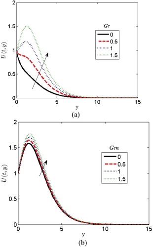The applied magnetic field strength $B_0$ gives rise to a resistive force called Lorentz force and it causes the motion of an electrically conducting fluid. It is clearly seen in Figure 6(b) that increasing the magnetic parameter causes a reduction in the velocity profile. The magnetic field induces currents in a moving conductive fluid. The induced currents polarize the fluid and change the magnetic field. Figure 7(a) depicts the effect of thermal Grashof number $Gr$ on the velocity profile. $Gr$ is the ratio of buoyancy to the viscous acting on the fluid. The velocity is coupled with temperature and concentration via thermal Grashof number and mass Grashof number as seen in Equation (8). Enhancement of thermal buoyancy force gives rise to the velocity. When the values of $Gr$ increase, it increases rapidly close to the plate and decreases the free stream velocity. This behaviour is shown in Figure 7(a). Figure 7(b) illustrates the influence of mass Grashof number $Gm$ on the velocity profile. It is evident from Figure 7(b) that the fluid velocity increases and the peak value is more distinctive because of the increase in the species buoyancy force.

Figure 2: Effects of (a) Prandtl number and (b) radiation parameter on velocity profiles.

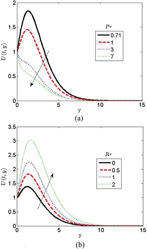
Figure 3: Effects of (a) Soret number and (b) Dufour number on velocity profiles.

Figure 4: Effects of (a) Viscoelastic fluid parameter and heat generation on velocity profiles.

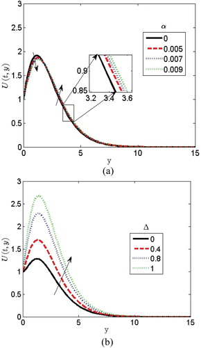
Figure 5: Effects of (a) Schmidt number and (b) chemical reaction parameter on the velocity profiles.

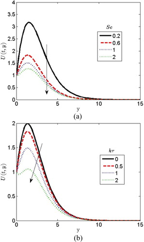
Figure 6: Effects of (a) Eckert number and (b) magnetic parameter on the velocity profiles.

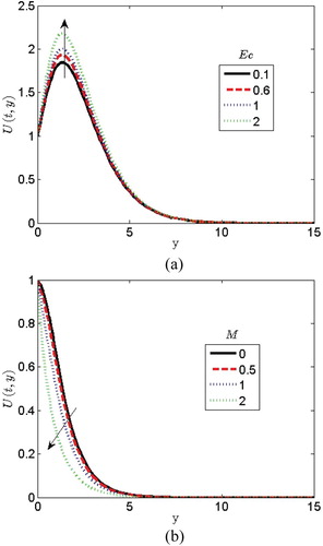
Figure 7: Effects of (a) thermal Grashof number and (b) mass Grashof number on velocity profiles.

4.2. Temperature profiles

From Figure 8(a) it is observed that the increase in $Pr$ decreases the temperature profile. It is noted that when $Pr<1$, the fluid in the hydrodynamic, thermal and concentration boundary layer is highly conducive. Also, small values of $Pr$ are equivalent to the enrichment of thermal conductivities. Prandtl number can be defined as the ratio of momentum diffusion to thermal diffusion. With the increase in $Pr$, the thermal diffusion decreases and therefore the thermal boundary layer becomes thinner. However, fluids with a very large $Pr$ and higher heat capacity tend to increase the rate of heat transfer and decreases the non-dimensional temperature. The effect of $Rr$ on the temperature profile is presented in Figure 8(b) shows that the temperature profile increases with an increase in $Rr$. 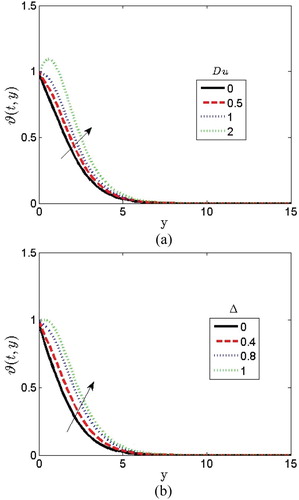When $Rr$ is raised the temperature of the fluid will increase causing an increase in the profile. Physically, increase in the radiation parameter brings heat energy to the thermal boundary layer. As a result of this, the heat energy gives room for more temperature and hereby increases the non-dimensional temperature. Figure 9(a) depicts the effect of Dufour parameter $Du$ on the temperature profile. The Dufour term explains the effect of concentration gradients as seen in Equation (9)(9) $\begin{array}{rl}& \frac{\mathrm{\partial }T}{\mathrm{\partial }{t}^{\mathrm{\prime }}}+v^{{}^{\mathrm{\prime }}\frac{\mathrm{\partial }T}{\mathrm{\partial }{y}^{\mathrm{\prime }}}}=\alpha \frac{{\mathrm{\partial }}^{2}T}{\mathrm{\partial }{y^{\mathrm{\prime }}}^2}-\frac{1}{\rho c_p}\frac{\mathrm{\partial }{q}_r}{\mathrm{\partial }{y}^{\mathrm{\prime }}}+\frac{\mu }{\rho c_p}{\left(\frac{\mathrm{\partial }{u}^{\mathrm{\prime }}}{\mathrm{\partial }{y}^{\mathrm{\prime }}}\right)}^2\\ & +\frac{D{K}_T{\mathrm{\partial }}^{2}C}{C_s{c}_p\mathrm{\partial }{y^{\mathrm{\prime }}}^2}+\frac{{\beta }^{\ast }u}{\rho c_p}\left(T_{\mathrm{\infty }}-T\right)+\frac{Q_0}{\rho c_p}\left(T-T_{\mathrm{\infty }}\right)\end{array}$(9) that plays a significant role in aiding the fluid flow and has the tendency to elevate the thermal energy in the boundary layer. From Figure 9(a), it is observed that as $Du$ increases it gives a rise in the temperature profile. The variation of heat generation/absorption coefficient parameter $\mathrm{\Delta }$ on the temperature profile is depicted in Figure 9(b). $\mathrm{\Delta }$ increases the temperature profile as seen in Figure 9(b) because the boundary layer gets thicker and the particles of the fluid become warm.

Figure 8: Effects of (a) Prandtl number and (b) radiation parameter on temperature profiles.

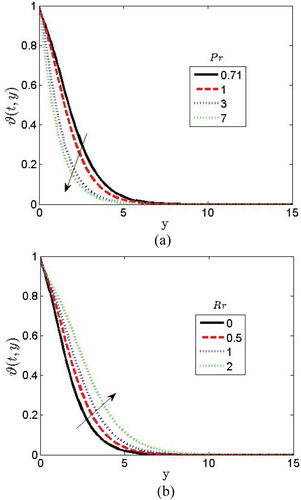
Figure 9: Effects of (a) Dufour number and (b) heat generation parameter on the temperature profiles.

4.3. Concentration profile

The variation of the Soret parameter $Sr$ on the concentration profile is depicted in Figure 10(a). The concentration profile rises when increasing the Soret parameter as shown in Figure 10(a). Figure 10(b) illustrates the variation of the Schmidt number $Sc$ on the concentration profile. It is obvious from Figure 10(b) that increasing the values of $Sc$ drastically decreases the concentration profile. The effect of the chemical reaction parameter $kr$ on the concentration profile is plotted in Figure 11. It is observed that the concentration profile decreases with increasing values of $kr$. The implication of this is that the buoyancy effects due to concentration and temperature difference are significant in the plate. The fluid motion is retarded on account of a chemical reaction. This implies that the destructive reaction $kr>0$ decreases the concentration field which weakens the buoyancy effects due to concentration gradients. Thus, the chemical reaction reduces the concentration, thereby increasing its concentration gradient and concentration flux (Tables 1–4).

Figure 10: Effects of (a) Soret number and (b) Schmidt number on the concentration profiles.

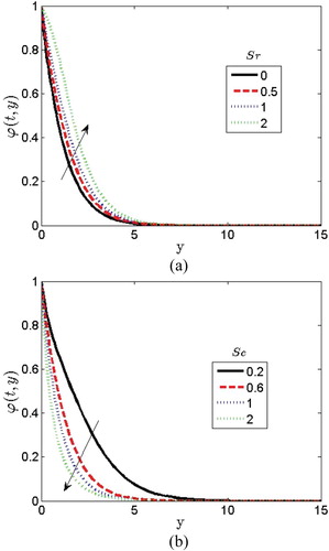
Figure 11: Effect of chemical reaction parameter on the concentration profile.

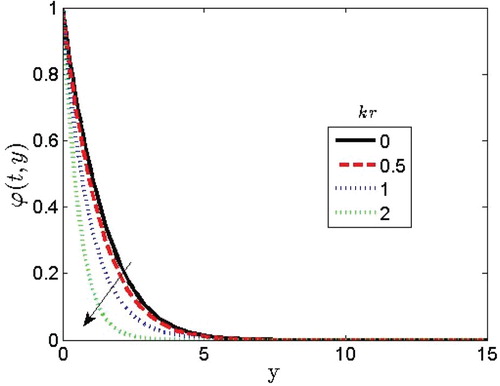
Table 1. Computational values for skin friction coefficient $\mathit{C}\mathit{f}$ and Nusselt number for various values of Schmidt number compared with [22] when $\mathit{\alpha }=\mathit{\delta }=\mathbf{\Delta }=\mathit{D}\mathit{u}=\mathit{S}\mathit{r}=0$.

	Present study		[22]
$Sc$	$Cf$	$Sh$	$Cf$	$Sh$
0.22	3.1067	0.4512	3.1068	0.4515
0.60	2.4546	0.8429	2.4548	0.8431
0.78	2.2766	1.0212	2.2767	1.0214
0.94	2.1539	1.1744	2.1540	1.1745

Table 2. Computational values for skin friction coefficient $\mathit{C}\mathit{f}$ and Nusselt number for various values of thermal radiation parameter compared with [23] when $\mathit{\alpha }=\mathit{\delta }=\mathbf{\Delta }=0$.

	Present study		[23]
$Rr$	$Cf$	${\vartheta }^{\mathrm{\prime }}\left(0\right)$	$Cf$	${\vartheta }^{\mathrm{\prime }}\left(0\right)$
0.0	1.7939	0.7452	1.7940	0.7455
0.4	1.9164	0.6532	1.9166	0.6533
0.8	2.0108	0.6049	2.0111	0.6051
1.0	2.0509	0.5889	2.0512	0.5892

Table 3. Computational values for skin friction coefficient $\mathit{C}\mathit{f}$, Nusselt number and Sherwood number with variation of Dufour parameter.

$Du$	$Cf$	$Nh$	$Sh$
0.0	0.9572	0.4174	0.6993
0.5	1.3468	0.5551	0.6993
1.0	1.7364	0.6928	0.6993

Table 4. Computational values for skin friction coefficient $\mathit{C}\mathit{f}$, Nusselt number and Sherwood number with variation of Soret parameter.

$Sr$	$Cf$	$Nh$	$Sh$
0.0	1.2097	0.6377	0.5353
0.5	1.5806	0.6377	0.6993
1.0	1.9514	0.6377	0.8633

5. Concluding remarks

In this paper, spectral relaxation method (SRM) is employed to solve a third-order-coupled partial differential equations that govern the effects of Soret and Dufour on MHD heat and mass transfer of a viscoelastic fluid pass over a semi-infinite vertical plate. Detailed explanation on SRM is discussed in the previous sections. Comparison of the present results is done with previously published work and was found to be in excellent agreement. The present results will be helpful in understanding the complex problems of MHD viscoelastic fluid over a semi-infinite vertical plate. The SRM is efficient and gives accurate results compared to other numerical methods used in the reviewed literature. Physically, the magnetic term in Equation (8) gives rise to the Lorentz force which interacts with the buoyancy force in the governing velocity and temperature fields. It slows down the motion of the fluid. The presence of the radiation term gives rise to the fluid temperature. When the radiation is further increased, there is a higher temperature which adds to the velocity of the fluid. The graphical representation is in Figure 2b and 8b of this study. The presence of thermal conductivity is very important in the study of the fluid phenomenon. An increase in the thermal conductivity reduces the velocity and the temperature field. From our numerical computations, we deduced the following:

1. When Dufour parameter is increased, the velocity profile as well as the temperature profiles increases.

2. Increasing the Soret parameter increases both the velocity and concentration profiles.

3. Effects of Soret and Dufour have opposite effect on the Nusselt and Sherwood number.

4. It was discovered that as the viscoelastic parameter increases, the velocity profile close to the plate decreases while far away from the plate it increases slightly.

5. The thermal Grashof number increases the hydrodynamic boundary layer when it is increased.

The effects of Soret–Dufour, thermal radiation and Walters’-B viscoelastic fluid as well as chemical reaction parameter on the flow profiles are significant in industrial and technological applications such as in coating of metals, crystal growth, electromagnetic pumps, power generators, MHD accelerators and reactor cooling.

Disclosure statement

No potential conflict of interest was reported by the authors.

ORCID

B. O. Falodun http://orcid.org/0000-0003-1020-1677

References

- Gbadeyan JA, Idowu AS, Ogunsola AW, et al. Heat and mass transfer for Soret and Dufour effect on mixed convection boundary layer flow over a stretching vertical surface in a porous medium filled with a viscoelastic fluid in the presence of magnetic field. Global Journal of Science Frontier Research. 2011;11(8):96–114.
- Choudhury R., Kumar Das S. Viscoelastic MHD free convective flow through porous media in presence of radiation and chemical reaction with heat and mass transfer. J Appl Fluid Mech. 2014;7(4):603–609.
- Rashidi MM, Ali M, Rostani B, Rostani P, et al. Heat and mass transfer for MHD viscoelastic fluid flow over a vertical stretching sheet with considering Soret and Dufour effects. Math Probl Eng. Article ID 861065, 2015;1–12. http://dx.doi.org/10.1155/2015/861065. doi: 10.1155/2015/861065
- Vedavathi N, Ramakrishna K, Jayarami RK. Radiation and mass transfer effects on unsteady MHD convective flow past an infinite vertical plate with Dufour and Soret effects. Ain Shams Eng J. 2014;6:363–371. doi: 10.1016/j.asej.2014.09.009
- Sharma BR, Aich A. Soret and Dufour effects on steady MHD flow in presence of heat source through a porous medium over a non-isothermal stretching sheet. IOSR J Math. 2016;12(1):53–60.
- Hayat T, Hina Z, Anum T, Ahmad A. Soret and Dufour effects on MHD peristaltic transport of Jeffrey fluid in a curved channel with convective boundary conditions. PLOS ONE. 2017;12(2) e0164854. DOI:10.1371/journal.pone.0164854.
- Iqbal M, Khalid S. Analysis of thermally developing laminar convection in the fined double-pipe. Heat Transf Res. 2013; 45(1): doi: 10.1615/HeatTransRes.2013006719.
- Ahmed F, Iqbal M. MHD power law fluid flow and heat transfer analysis through Darcy Brinkamn porous media in annular sector. Int J Mech Sci. 130:508–517. doi: 10.1016/j.ijmecsci.2017.05.042
- Ahmed F, Iqbal M, Sher Akbar. Numerical study of forced convective power law fluid flow through an annulus sector duct. Eur Phys J Plus. 131:341. https://doi.org/10.1140/epjp/i.16341-x doi: 10.1140/epjp/i2016-16341-x
- Iqbal M, Afag Hamna. Fluid flow and heat transfer through an annular sector duct filled with porous media. J Porous Media. 18(7):679–687. DOI:10.1615/JPorMedia.v18.i7.30.
- Iqbal M, Ahmed F, Rashidi MM. Simulation of MHD forced convection heat transfer through annular sector duct. J Thermophys Heat Transfer. 32(2):469–474. doi: 10.2514/1.T5293
- Selimefendigil F, Oztop H.F. Role of magnetic field and surface corrugation on natural convection in a nanofluid filled 3D trapezoidal cavity. Int Commun Heat and Mass. 2018; 95: 182–196. doi: 10.1016/j.icheatmasstransfer.2018.05.006
- Selimefendigil F, Oztop HF. Conjugate natural convection in a nanofluid filled partitioned horizontal annulus formed by two isothermal cylinder surfaces under magnetic field. Int J Heat Mass Transf. 2017; 108:156–171. doi: 10.1016/j.ijheatmasstransfer.2016.11.080
- Selimefendigil F, Oztop HF, Chamkha AJ. Fluid structure-magnetic field lid-driven cavity with flexible side wall. Eur J Mech-B/Fluids. 2017; 61(1):77–85. doi: 10.1016/j.euromechflu.2016.03.009
- Selimefendigil F, Oztop HF. Analysis of MHD mixed convection in a flexible walled and nanofluids filled lid-driven cavity with volumetric heat generation. Int J Mech Sci 2016; 118, 113–124. doi: 10.1016/j.ijmecsci.2016.09.011
- Rashidi MM, Momoniat E, Rostani B. Analytic approximate solutions for MHD boundary-layer viscoelastic fluid flow over continuously moving stretching surface by homotopy analysis method with two auxiliary parameters. J Appl Math. Article ID 780415, 2012;1–19. DOI:10.1155/2012/780415.
- Sivaraj R, Kumar BR. Chemically reacting dusty viscoelastic fluid flow in an irregular channel with convective boundary. Ain Shams Eng J. 2013;4:93–101. doi: 10.1016/j.asej.2012.06.005
- Manglesh A, Gorla. The effects of thermal radiation, chemical reaction and rotation on unsteady MHD viscoelastic slip flow. Global Journal of Science Frontier Research Mathematics and Decision Sciences. 2012;12(14):1–15.
- Kumar BR, Sivaraj. Heat and mass transfer in MHD viscoelastic fluid flow over a vertical cone and flat plate with variable viscosity. Int J Heat Mass Transf. 2013;56(1):370–379. doi: 10.1016/j.ijheatmasstransfer.2012.09.001
- Eswaramoorthi S, Bhuvaneswari M, Sivasankaran S, et al. Effect of radiation on MHD convective flow and heat transfer of a viscoelastic fluid over a stretching surface. Procedia Eng. 2015;127:916–923. doi: 10.1016/j.proeng.2015.11.364
- Madhu M, Kishan N. Finite element analysis of MHD viscoelastic nanofluid flow over a stretching sheet with radiation. Procedia Eng. 2015;127:432–439. doi: 10.1016/j.proeng.2015.11.393
- Rao VS, Baba LA, Raju RS. Finite element analysis of radiation and mass transfer flow past semi-infinite moving vertical plate with viscous dissipation. J Appl Fluid Mech. 2013;6:321–329.
- Alao FI, Fagbade AI, Falodun BO. Effects of thermal radiation, Soret and Dufour on an unsteady heat and mass transfer flow of a chemically reacting fluid past a semi-infinite vertical plate with viscous dissipation. J Nigerian Math Soc. 2016;35:142–158. doi: 10.1016/j.jnnms.2016.01.002
- Walters K. Non-Newtonian effects in some elastico-viscous liquids whose behaviour at small rates of shear is characterized by a general linear equations of state. Quantum J Mech Appl Math. 1962;15:63–76. doi: 10.1093/qjmam/15.1.63
- Motsa SS. New iterative methods for solving nonlinear boundary value problems. Fifth annual workshop on computational applied mathematics and mathematical modeling in fluid flow. School of mathematics, statistics and computer science, Pietermaritzburg Campus 2012;9–13.
- Motsa SS, Dlamini PG, Khumalo M. Spectral relaxation method and spectral quasilinearization method for solving unsteady boundary layer flow problems. Adv Math Phys. Article ID 341964, 2014;1–12. http://dx.doi.org/10.1155/2014/341964.