Effect of joule heating and MHD on peristaltic blood flow of Eyring–Powell nanofluid in a non-uniform channel

Abstract

This paper examines the effect of joule heating and MHD on peristaltic blood flow of a Eyring–Powell nanofluid in a non-uniform channel. The transport equations involve the combined effects of Brownian and Thermophoresis diffusion of nanoparticles. The mathematical modelling is carried out by utilizing long wavelength and low Reynolds number assumptions. The energy equation is modelled by taking joule heating effect. The resulting nonlinear system of partial differential equations is solved for the stream function, velocity, pressure gradient, concentration and temperature distributions with the help of the Homotopy Analysis Method. The effect of various physical parameters on the flow characteristics is shown and discussed with the help of graphs. Pressure gradient gives opposite behaviour with increasing values of Eyring–Powell fluid parameters A and B. Pressure gradient decreases by increasing Hartman number and joule heating. Nanoparticle concentration increases with increasing thermophoresis parameter, but the reverse trend is observed with the effect of Brownian motion parameter.

KEYWORDS:

• Peristalsis
• Eyring–Powell fluid
• thermophoresis and Brownian diffusion
• MHD
• joule heating

Nomenclature

$\tilde{u},\tilde{v}$	=	velocity components (m/s)
$\tilde{x},\tilde{y}$	=	Cartesian coordinates (m)
$\tilde{t}$	=	time (s)
$\tilde{p}$	=	pressure in fixed frame (N/m2)
$B_0$	=	magnetic field
$\beta$,$c^{\ast }$	=	material parameters
$\mathrm{\Phi }$	=	constant heat addition/absorption
$\kappa$	=	volume expansion coefficient
$\tilde{T}$	=	temperature of the fluid (K)
$\tilde{C}$	=	nanoparticle concentration
$D_{\mathrm{B}}$	=	Brownian diffusion coefficient
$D_{\mathrm{T}}$	=	Thermophoresis diffusion
$T_{\mathrm{m}}$	=	fluid mean temperature
$Re$	=	Reynolds number
Pr	=	Prandtl number
Gr, Qr	=	Grashof numbers due to local temperature and local nanoparticles concentration, respectively
Ec	=	Eckert number
Br	=	Brinkman number
$\tilde{S}$	=	stress tensor

Greek symbols

µ	=	dynamic viscosity (Ns/m2)
$\sigma$	=	electrical conductivity of the fluid (S/m)
$\delta$	=	wave number (m−1)
${\rho }_f$	=	density of the fluid (kg/m3)
$k^{\ast }$	=	thermal conductivity
$\alpha$	=	amplitude ratio (m)
$\lambda$	=	wavelength (m)

1. Introduction

The peristaltic transport of Eyring–Powell nanofluid in a non-uniform channel is an important problem in engineering, industrial and biological applications. It is useful for the description of the progressive wave contraction along a channel or tube. In particular, the mechanism involved in swallowing food through esophagus, urine transport from kidney to bladder through the ureter, movement of chime in the gastrointestinal tract, vasomotion of small blood vessels and the locomotion of some warms, etc. Peristaltic pump is also used in roller and finger pump. Such devices are used to pump the blood, in bypass surgery it is used to circulate the blood in heart lung machine, slurries is to prevent the transport of fluid from coming in contact with mechanical part of the pump. The word peristaltic comes from the Greek word as “peristaltikos” which means clutching and compressing. Latham [1] was the first who investigated the fluid motion in peristaltic pump. After his first investigation, a large number of researchers and scientist focus their attentions to study the peristaltic flows considering Newtonian and non-Newtonian fluids [2–7]. Bhatti et al. [8] have studied the study of variable magnetic field on the peristaltic flow of Jeffrey fluid in a non-uniform rectangular duct having compliant walls. Further, nanofluid is a fluid containing nanometer-sized particles called nanoparticle. The nanoparticles used in nanofluids are typically made of metals (Al, Cu), oxides (ceramics, Al₂O₃, CuO); non-metal like graphite and carbon nanotubes, nanofibres, droplet, nanosheet, etc. Chio [9] was the first to introduce the word nanofluid that represents the fluid in which nanoscale particles (diameter less than 100 nm) are suspended in the base fluid. Recent articles on the nanofluid are cited in [10–13].

Powell and Eyring proposed a new fluid model in 1944 known as Eyring–Powell fluid model [14]. Viscoelastic fluids in physiology and industry have a prominent place. The Eyring–Powell nanofluid is one such model which is advantageous to recover accurate results of viscous nanofluid at low and high shear rates. At low shear rates less than 100 s⁻¹, the best example of Eyring–Powell nanofluid is human blood. Possibly the complex mathematical description of this model in flexible curved channel averts the study of nanoparticles subject to Eyring–Powell fluid [15]. Further investigation of mixed convection peristaltic flow of Eyring–Powell nanofluid with magnetic field in a non-uniform channel by Asha and Sunitha [16]. Nooren and Qasim [17] studied the peristaltic flow of MHD Eyring–Powell fluid in a channel. Recent articles on the peristaltic transport of Eyring–Powell fluid are cited in [18–21]. Peristalsis in connection with nanofluids has application in biomedicines, i.e. cancer treatment, radio therapy, etc.

Peristaltic blood flow has gained considerable attention because of its major importance in physiological. The velocity of blood flow in the human body is different depending on what type of vessels it is flowing through. Velocity is indirectly related to the cross-sectional area of the vascular bed, so when the cross-sectional area is high (i.e. in capillaries) then the speed of blood flow decreases dramatically. Blood flow follows the laws of hydrodynamics where speed is proportional to pressure difference, fluidity, radius of the tube. When blood flows from heart to various organs it passes through aorta to artery to arterioles to capillaries. Capillaries have very small diameter but as arteriole is divided into many capillaries, the overall diameter increases, so blood volume decreases. So through flow of blood from aorta to capillaries the speed of flow gradually decreases and flow gradually become streamline. Recently, peristaltic flow with magnetic particles grabbed the attention of several researchers due to its emerging applications in magnetic drug targeting [22], pumping of blood, reduction of bleeding during surgery, continue casting process, hyperthermia, magnetic resonance imaging (MRI) and Magneto-therapy, etc. Moreover, in biomedical engineering,ferrofluid is beneficial for an experimental treatment of cancer disease (known as targeted magnetic hyperthermia). Furthermore, magneto-hydrodynamic (MHD) flow and heat transfer towards moving or fixed flat surface have become a vibrant problem in the current field and huge applications in the field of engineering problems, for instance, petroleum engineering, plasma studies, geothermal energy abstractions, aerodynamics and much more. Bhatti et al. [23] have studied the Combine effects of Magnetohydrodynamics (MHD) and partial slip on peristaltic Blood flow of Ree-Eyring fluid with wall properties. Particularly, to regulate the behaviour of boundary layer, numerous artificial approaches have been established in references [24–26]. Joule heating effect cannot be ignored when strong magnetic field is applied. There are many practical uses of joule heating such as conductors in electronics, electric stoves and other electric heaters, power lines, fuses. The study of heat and mass transfer with joule heating on MHD peristaltic blood flow under the influence of hall effect was given by Bhatti et al. [27]. Recent attempts on mixed convection peristaltic flow with joule effect can be seen in [28,29].

As far the best of author’s knowledge, the effect of joule heating on MHD peristaltic blood flow of Eyring–Powell nanofluid in a non-uniform channel has not been studied yet. However, Anum et al. [12] studied the mixed convection peristaltic flow of Eyring–Powell nanofluid in a curved channel with compliant walls, but did not consider the effect of joule heating. The prime object of the present attempt is to explore the ideas of MHD and joule heating on the peristaltic blood flow by considering the Eyring–Powell nanofluid. The present study has numerous applications in biomedical engineering. In most medical therapies, MHD with joule heating plays an important role to modulate the blood and to reduce the pain of human body (like in laparoscopic treatment). This paper is organized in the following fashion. In Section 1, the mathematical formulation of the problem is constructed by employing the wave frame and then reduced by assumptions of long wavelength and low Reynolds number approximation. In Section 2, solutions for velocity, temperature and concentration are obtained by using the Homotopy Analysis Method (HAM) [30,31]. This method is a general approximate analytic solution, used to obtain series solutions of linear/nonlinear equations. This method is valid for the nonlinear problem, contains small or large physical parameters. The method provides great freedom in choosing initial approximation and auxiliary linear operators. By means of choosing such approximation and operators, any complicated nonlinear problems can be solved by transforming into linear subproblems. In the last section, the effects of various physical parameters on pressure gradient, frictional force, concentration and temperature are analysed through graphs.

2. Mathematical formulation

Let us consider the peristaltic blood flow of Eyring–Powell nanofluid through a two-dimensional non-uniform channel with the sinusoidal wave propagating towards down its walls. The nanofluid is electrically conducting by an external magnetic field$B_0$ and the effect of joule heating. Here we consider the Cartesian coordinate system ($\tilde{X},\tilde{Y}$) such that $\tilde{X}$-axis is considered along the centre line in the direction of wave propagation and $\tilde{Y}$-axis is transverse. The geometry of the wall surface can be written as (1) $\tilde{h}\left(\tilde{X},\tilde{t}\right)=a\left(\tilde{X}\right)+bsin\left(\frac{2\pi }{\lambda }\left(\tilde{X}-c\tilde{t}\right)\right).$(1)

Here $a\left(\tilde{X}\right)=a_{20}+k\tilde{X}$ is the channel half-width, $\lambda$ is the wavelength, $\tilde{t}$ is the time and $b$ represents the wave amplitude. The velocity components $\tilde{U}$ and $\tilde{V}$ along the $\tilde{X}$ and $\tilde{Y}$ directions, respectively, in the fixed frame, the velocity field $V$ is taken as (2) $V=\left[\tilde{U}\left(\tilde{X},\tilde{Y},\tilde{t}\right),\tilde{V}\left(\tilde{X},\tilde{Y},\tilde{t}\right),0\right].$(2)

The shear of non-Newtonian fluid is considered to the study of Eyring–Powell fluid model. The stress tensor of Eyring–Powell fluid model is given by (3) $\tilde{S}=\mu \mathrm{\nabla }\tilde{V}+\frac{1}{\beta }{\sinh }^{-1}\left(\frac{1}{c^{\ast }}\mathrm{\nabla }\tilde{V}\right),$(3) where $\mu$ is the coefficient of shear viscosity, $\beta$ and $c^{\ast }$ are the material constant of Eyring–Powell fluid. The term $\left({\sinh }^{-1}\right)$ is approximated using the second-order approximation of the hyperbolic sine function as follows: (4) ${\sinh }^{-1}\left(\frac{1}{c^{\ast }}\mathrm{\nabla }\tilde{V}\right)\approx \frac{1}{c^{\ast }}-\frac{1}{6}{\left(\frac{1}{c^{\ast }}\mathrm{\nabla }\tilde{V}\right)}^3,\left|\frac{1}{c^{\ast }}\mathrm{\nabla }\tilde{V}\right|\ll 1.$(4) The governing equations for the Eyring–Powell nanofluid can be written as follows [17]:

The continuity equation: (5) $\frac{\mathrm{\partial }\tilde{U}}{\mathrm{\partial }\tilde{X}}+\frac{\mathrm{\partial }\tilde{U}}{\mathrm{\partial }\tilde{Y}}=0.$(5) The momentum equation: (6) $\begin{array}{rl}& {\rho }_f\left(\frac{\mathrm{\partial }\tilde{U}}{\mathrm{\partial }\tilde{t}}+\tilde{U}\frac{\mathrm{\partial }\tilde{U}}{\mathrm{\partial }\tilde{X}}+\tilde{V}\frac{\mathrm{\partial }\tilde{U}}{\mathrm{\partial }\tilde{Y}}\right)\\ & =-\frac{\mathrm{\partial }\tilde{p}}{\mathrm{\partial }\tilde{X}}+\left(\mu +\frac{1}{\beta c^{\ast }}\right)\left(\frac{{\mathrm{\partial }}^2\tilde{U}}{\mathrm{\partial }{\tilde{X}}^2}+\frac{{\mathrm{\partial }}^2\tilde{U}}{\mathrm{\partial }{\tilde{Y}}^2}\right)-\sigma {B_0}^2\tilde{U}\\ & -\frac{1}{2\beta c^{\ast 3}}\left\{{\left(\frac{\mathrm{\partial }\tilde{U}}{\mathrm{\partial }\tilde{X}}\right)}^2+{\left(\frac{\mathrm{\partial }\tilde{U}}{\mathrm{\partial }\tilde{Y}}\right)}^2+2\left(\frac{\mathrm{\partial }\tilde{U}}{\mathrm{\partial }\tilde{X}}\right)\left(\frac{\mathrm{\partial }\tilde{U}}{\mathrm{\partial }\tilde{Y}}\right)\right\}\\ & \times \left(\frac{{\mathrm{\partial }}^2\tilde{U}}{\mathrm{\partial }{\tilde{X}}^2}+\frac{{\mathrm{\partial }}^2\tilde{U}}{\mathrm{\partial }{\tilde{Y}}^2}\right)+{\rho }_{f}g\kappa \left(\tilde{T}-{\tilde{T}}_0\right)+{\rho }_{f}g\kappa \left(\tilde{C}-{\tilde{C}}_0\right),\end{array}$(6) (7) $\begin{array}{rl}& {\rho }_f\left(\frac{\mathrm{\partial }\tilde{V}}{\mathrm{\partial }\tilde{t}}+\tilde{U}\frac{\mathrm{\partial }\tilde{V}}{\mathrm{\partial }\tilde{X}}+\tilde{V}\frac{\mathrm{\partial }\tilde{V}}{\mathrm{\partial }\tilde{Y}}\right)\\ & =-\frac{\mathrm{\partial }\tilde{p}}{\mathrm{\partial }\tilde{Y}}+\left(\mu +\frac{1}{\beta c^{\ast }}\right)\left(\frac{{\mathrm{\partial }}^2\tilde{V}}{\mathrm{\partial }{\tilde{X}}^2}+\frac{{\mathrm{\partial }}^2\tilde{V}}{\mathrm{\partial }{\tilde{Y}}^2}\right)\\ & -\frac{1}{2\beta c^{\ast 3}}\left\{{\left(\frac{\mathrm{\partial }\tilde{V}}{\mathrm{\partial }\tilde{X}}\right)}^2+{\left(\frac{\mathrm{\partial }\tilde{V}}{\mathrm{\partial }\tilde{Y}}\right)}^2+2\left(\frac{\mathrm{\partial }\tilde{V}}{\mathrm{\partial }\tilde{X}}\right)\left(\frac{\mathrm{\partial }\tilde{V}}{\mathrm{\partial }\tilde{Y}}\right)\right\}\\ & \times \left(\frac{{\mathrm{\partial }}^2\tilde{V}}{\mathrm{\partial }{\tilde{X}}^2}+\frac{{\mathrm{\partial }}^2\tilde{V}}{\mathrm{\partial }{\tilde{Y}}^2}\right).\end{array}$(7)

The energy equation: (8) $\begin{array}{rl}& (\rho c{)}_f\left(\frac{\mathrm{\partial }\tilde{T}}{\mathrm{\partial }\tilde{t}}+\tilde{U}\frac{\mathrm{\partial }\tilde{T}}{\mathrm{\partial }\tilde{X}}+\tilde{V}\frac{\mathrm{\partial }\tilde{T}}{\mathrm{\partial }\tilde{Y}}\right)\\ & =k^{\ast }\left(\frac{{\mathrm{\partial }}^2\tilde{T}}{\mathrm{\partial }{\tilde{X}}^2}+\frac{{\mathrm{\partial }}^2\tilde{T}}{\mathrm{\partial }{\tilde{Y}}^2}\right)+(\rho c{)}_p{D}_B\left(\frac{\mathrm{\partial }\tilde{C}}{\mathrm{\partial }\tilde{X}}+\frac{\mathrm{\partial }\tilde{C}}{\mathrm{\partial }\tilde{Y}}\right)\\ & \times \left(\frac{\mathrm{\partial }\tilde{T}}{\mathrm{\partial }\tilde{X}}+\frac{\mathrm{\partial }\tilde{T}}{\mathrm{\partial }\tilde{Y}}\right)+(\rho c{)}_p\frac{D_T}{T_m}{\left(\frac{{\mathrm{\partial }}^2\tilde{T}}{\mathrm{\partial }{\tilde{X}}^2}+\frac{{\mathrm{\partial }}^2\tilde{T}}{\mathrm{\partial }{\tilde{Y}}^2}\right)}^2\\ & +\mathrm{\Phi }+\sigma {B_0}^2{\tilde{U}}^2.\end{array}$(8) The concentration equation: (9) $\begin{array}{rl}& \frac{\mathrm{\partial }\tilde{C}}{\mathrm{\partial }\tilde{t}}+\tilde{U}\frac{\mathrm{\partial }\tilde{C}}{\mathrm{\partial }\tilde{X}}+\tilde{V}\frac{\mathrm{\partial }\tilde{C}}{\mathrm{\partial }\tilde{Y}}\\ & =D_B\left(\frac{{\mathrm{\partial }}^2\tilde{C}}{\mathrm{\partial }{\tilde{X}}^2}+\frac{{\mathrm{\partial }}^2\tilde{C}}{\mathrm{\partial }{\tilde{Y}}^2}\right)+\frac{D_T}{T_m}\left(\frac{{\mathrm{\partial }}^2\tilde{T}}{\mathrm{\partial }{\tilde{X}}^2}+\frac{{\mathrm{\partial }}^2\tilde{T}}{\mathrm{\partial }{\tilde{Y}}^2}\right),\end{array}$(9) where $\tilde{p}$ is the pressure, ${\rho }_f$ is the density of the fluid, $\sigma$ is the electrical conductivity of the fluid, $B_0$ is the applied magnetic field, $\mathrm{\Phi }$ is the constant heat addition/absorption, $g$ is the acceleration due to gravity, $\kappa$ is the volume expansion coefficient, $\tilde{T}$ is the temperature of the fluid, $\tilde{C}$ is the nanoparticle concentration, $(\rho c{)}_f$ is the heat capacity of the fluid, $k^{\ast }$ is the thermal conductivity, $(\rho c{)}_p$ is the effective heat capacity of the nanoparticle material, $D_{\mathrm{B}}$ is the Brownian diffusion coefficient, $D_{\mathrm{T}}$ is thermophoresis diffusion and $T_{\mathrm{m}}$ is the fluid mean temperature.

The relations between the laboratory and wave frame are introduced through (10) $\begin{array}{ll}\tilde{x}=\tilde{X}-c\tilde{t},& \tilde{y}=\tilde{Y},\\ \tilde{u}(\tilde{x},\tilde{y})=\tilde{U}-c,& \tilde{v}(\tilde{x},\tilde{y})=\tilde{V},\end{array}$(10) where $(\tilde{u},\tilde{v})$ and $(\tilde{x},\tilde{y})$ indicate the velocity components and coordinates in the wave frame.

Introducing the velocity field in terms of stream functions can be written as $\left(u=\frac{\mathrm{\partial }\psi }{\mathrm{\partial }y},v=-\delta \frac{\mathrm{\partial }\psi }{\mathrm{\partial }x}\right)$. The corresponding boundary conditions for the above problem is given by (11) $\left.\begin{array}{l}\tilde{\psi }=0,\tilde{u}=\frac{\mathrm{\partial }\tilde{\psi }}{\mathrm{\partial }\tilde{y}}=0,\tilde{T}={\tilde{T}}_0,\tilde{C}={\tilde{C}}_0\text{at}\tilde{y}=0,\\ \tilde{\psi }=q,\tilde{u}=\frac{\mathrm{\partial }\tilde{\psi }}{\mathrm{\partial }\tilde{y}}=-c,\tilde{T}={\tilde{T}}_1,\tilde{C}={\tilde{C}}_1\text{at }\tilde{y}=\tilde{h}\\ =a\left(\tilde{x}\right)+b\sin \frac{2\pi }{\lambda }\left(\tilde{x}\right).\end{array}\right\}$(11)

Introducing the following non-dimensional quantities: (12) $\left.\begin{array}{l}\psi =\frac{\tilde{\psi }}{ca},B=\frac{1}{\mu \beta c^{\ast }},A=\frac{B{c}^2}{2a^2{c}^{\ast 2}},X=\frac{\tilde{X}}{\lambda },x=\frac{\tilde{x}}{\lambda },\\ Y=\frac{\tilde{Y}}{a},y=\frac{\tilde{y}}{a},t=\frac{c\tilde{t}}{\lambda },p=\frac{a^2\tilde{p}}{c\lambda \mu },v=\frac{\tilde{v}}{c},\\ \delta =\frac{a}{\lambda },u=\frac{\tilde{u}}{c},\mathrm{Re}=\frac{2{\rho }_{f}ca}{\mu },M=\sqrt{\frac{\sigma }{\mu }}{B}_{0}a,\\ {\beta }^{\ast }=\frac{k^{\ast }}{{\left(\rho c\right)}_f},Pr=\frac{\mu }{\beta \ast },F=\frac{q}{ca}Gr=\frac{{\rho }_{f}gk{a}^2\left({\tilde{T}}_1-{\tilde{T}}_0\right)}{c\mu },\\ Qr=\frac{{\rho }_{f}gk{a}^2\left({\tilde{C}}_1-{\tilde{C}}_0\right)}{c\mu },Nb=\frac{{\left(\rho c\right)}_p{D}_B\left({\tilde{C}}_1-{\tilde{C}}_0\right)}{{\left(\rho c\right)}_f\mu },\\ Nt=\frac{{\left(\rho c\right)}_p{D}_T\left({\tilde{T}}_1-{\tilde{T}}_0\right)}{{\left(\rho c\right)}_f{T}_m\mu },Q_0=\frac{a^2\mathrm{\Phi }}{\left({\tilde{T}}_1-{\tilde{T}}_0\right){\left(\rho c\right)}_f},\\ E_c=\frac{c^2}{{\left(\rho c\right)}_p\left({\tilde{T}}_1-{\tilde{T}}_0\right)},Br=Pr{E}_c,\mathrm{\Omega }=\frac{\tilde{C}-{\tilde{C}}_0}{{\tilde{C}}_1-{\tilde{C}}_0},\\ \theta =\frac{\tilde{T}-{\tilde{T}}_0}{{\tilde{T}}_1-{\tilde{T}}_0},h=\frac{\tilde{h}}{a_{20}}=1+\frac{\lambda kx}{a_{20}}\\ +\alpha \sin 2\pi x,\alpha =\frac{b}{a_{20}}.\end{array}\right\}$(12)

The non-dimensional symbols of the above-mentioned quantities are as follows: A and B are the non-dimensional Eyring–Powell fluid parameters, $Pr$ is the Prandtl number, Gr and Qr are the Grashof numbers corresponding to the local temperature and local nanoparticles mass transfer respectively, Nb is the Brownian motion parameter, Nt is the Thermophoresis parameter, the Hartmann number M, $Q_0$ is the heat generation parameter, Br is the Brinkman number and Ec is the Eckert number, the temperature distribution $\theta$, $\mathrm{\Omega }$ is the mass concentration, p is the dimensionless pressure, $\psi$ is the stream function, x is the non-dimensional axial coordinate, y is the non-dimensional transverse coordinate, (u, v) is the velocity components, F is the dimensionless average flux in the wave frame, µ is the dynamic viscosity and $\alpha$is the amplitude ratio.

The nonlinear terms in the momentum equation are determined to be zero $\left(Re{\delta }^2\right)$, where $Re=\frac{2{\rho }_{f}ca}{\mu }$ is the Reynolds number and $\delta =\frac{a}{\lambda }$ is the wave number and using non-dimensional quantities. Introducing the velocity fields in terms of stream functions $\left(u=\frac{\mathrm{\partial }\psi }{\mathrm{\partial }y},v=-\delta \frac{\mathrm{\partial }\psi }{\mathrm{\partial }x}\right)$ with long wavelength and low Reynolds number approximation, the basic equations (1)–(12) reduce to (13) $\begin{array}{rl}\frac{\mathrm{\partial }p}{\mathrm{\partial }x}& =(1+B)\frac{{\mathrm{\partial }}^3\psi }{\mathrm{\partial }{y}^3}-A{\left(\frac{{\mathrm{\partial }}^2\psi }{\mathrm{\partial }{y}^2}\right)}^2\frac{{\mathrm{\partial }}^3\psi }{\mathrm{\partial }{y}^3}\\ & -M^2\frac{\mathrm{\partial }\psi }{\mathrm{\partial }y}+Gr\theta +Br\mathrm{\Omega },\end{array}$(13) (14) $\frac{\mathrm{\partial }p}{\mathrm{\partial }y}=0,$(14) (15) $\begin{array}{rl}& \frac{{\mathrm{\partial }}^2\theta }{\mathrm{\partial }{y}^2}+PrNb\frac{\mathrm{\partial }\theta }{\mathrm{\partial }y}\frac{\mathrm{\partial \Omega }}{\mathrm{\partial }y}+PrNt{\left(\frac{\mathrm{\partial }\theta }{\mathrm{\partial }y}\right)}^2\\ & +Pr{Q}_0+Br{M}^2{u}^2=0,\end{array}$(15) (16) $\frac{{\mathrm{\partial }}^2\mathrm{\Omega }}{\mathrm{\partial }{y}^2}+\frac{Nt}{Nb}\frac{{\mathrm{\partial }}^2\theta }{\mathrm{\partial }{y}^2}=0.$(16)

The corresponding dimensionless boundary conditions can be written in the following form: (17) $\left.\begin{array}{rl}& \psi =0,\frac{{\mathrm{\partial }}^2\psi }{\mathrm{\partial }{y}^2}=0,\theta =0,\mathrm{\Omega }=0\text{at}y=0,\\ & \psi =F,\frac{\mathrm{\partial }\psi }{\mathrm{\partial }y}=-1,\theta =1,\mathrm{\Omega }=1\text{at}y=h\\ & =1+\frac{\lambda kx}{a_{20}}+\alpha \sin 2\pi x,\end{array}\right\}$(17) where the dimensionless time mean flow rate $F$ is the wave frame is related to the dimensionless time mean flow rate in the laboratory frame as follows: (18) $\mathrm{\Theta }=F+1,F={\int }_0^h\frac{\mathrm{\partial }\psi }{\mathrm{\partial }y}\text{d}y,$(18) here $\mathrm{\Theta }=\frac{Q}{ca}\text{and }F=\frac{q}{ca}$ are the dimensionless time mean flow in a fixed and wave form respectively.

3. Method of solution

Analysing the governing Equations (13)–(16) and corresponding boundary conditions (17), it is to find that the solution is an odd function (13) equation and even functions of (15)–(16). Besides, noticing that Equations (13)–(16) contain the term y, it is convenient to express u(y), $\theta \left(y\right)$ and $\mathrm{\Omega }\left(y\right)$ by power polynomials. So, we consider the auxiliary linear operators by using HAM. For HAM solutions, we calculate the initial guesses and auxiliary linear operators in the following form: (19) ${\psi }_0\left(y\right)=\frac{y\left(4F{h}^3-F{y}^3+h^4-h{y}^3\right)}{3h^4},$(19) (20) ${\theta }_0\left(y\right)=\frac{y}{h},$(20) (21) ${\mathrm{\Omega }}_0\left(y\right)=\frac{y}{h}.$(21)

The corresponding auxiliary linear operators are (22) $L_{\psi }=\frac{{\mathrm{\partial }}^5}{\mathrm{\partial }{y}^5},L_{\theta }=\frac{{\mathrm{\partial }}^2}{\mathrm{\partial }{y}^2},L_{\mathrm{\Omega }}=\frac{{\mathrm{\partial }}^2}{\mathrm{\partial }{y}^2}$(22) with property (23) $\begin{array}{rl}& L_{\psi }\left[C_1+C_{2}y+C_3\frac{y^2}{2}+C_4\frac{y^3}{6}+C_5\frac{y^4}{24}\right]=0,\\ & L_{\theta }\left[C_1+C_{2}y\right]=0,L_{\mathrm{\Omega }}\left[C_1+C_{2}y\right]=0,\end{array}$(23) where $C_1,C_2,C_3,C_{4}and{C}_5$ are arbitrary constants, the zeroth-order deformation equations are (24) $\left(1-q\right)L_{\psi }\left[\psi \left(y,q\right)-{\psi }_0\left(y,q\right)\right]=q{H}_{\psi }{h}_{\psi }N\left[\psi \left(y,q\right)\right],$(24) (25) $\left(1-q\right)L_{\theta }\left[\theta \left(y,q\right)-{\theta }_0\left(y,q\right)\right]=q{H}_{\theta }{h}_{\theta }N\left[\theta \left(y,q\right)\right],$(25) (26) $\left(1-q\right)L_{\mathrm{\Omega }}\left[\mathrm{\Omega }\left(y,q\right)-{\mathrm{\Omega }}_0\left(y,q\right)\right]=q{H}_{\mathrm{\Omega }}{h}_{\mathrm{\Omega }}N\left[\mathrm{\Omega }\left(y,q\right)\right],$(26) where $q\in \left[0,1\right]$ is the embedding parameter, $h_{\psi },h_{\theta }\text{and}{h}_{\mathrm{\Omega }}$ are auxiliary parameters, L is an auxiliary linear operator, $H_{\psi ,}{H}_{\theta }\text{and}{H}_{\mathrm{\Omega }}$ are auxiliary functions, N is a nonlinear operator, $\psi \left(y,q\right),\theta \left(y,q\right)\text{and}\mathrm{\Omega }\left(y,q\right)$ are unknown functions, ${\psi }_0\left(y,q\right),{\theta }_0\left(y,q\right)\text{and}{\mathrm{\Omega }}_0\left(y,q\right)$ are initial approximations of$\psi \left(y,q\right),\theta \left(y,q\right)\text{and}\mathrm{\Omega }\left(y,q\right)$.

From Equations (24)–(26), we can easily find the system of equations with their relevant boundary conditions. According to the methodology of the HAM, the solutions are given by (27) $\theta \left(y,q\right)={\theta }_0+h_{\theta }{\theta }_1+{h_{\theta }}^2\theta {}_2+\cdots$(27) (28) $\mathrm{\Omega }\left(y,q\right)={\mathrm{\Omega }}_0+h_{\mathrm{\Omega }}{\mathrm{\Omega }}_1+{h_{\mathrm{\Omega }}}^2\mathrm{\Omega }{}_2+\cdots$(28) (29) $\psi \left(y,q\right)={\psi }_0+h_{\psi }{\psi }_1+{h_{\psi }}^2\psi {}_2+\cdots$(29)

The solutions for velocity $\left(u=\frac{\mathrm{\partial }\psi }{\mathrm{\partial }y}\right)$, temperature and concentration are evaluated using Equations (27)–(29) we get (30) $\begin{array}{rl}u\left(y,q\right)& =\left(\frac{1}{3}+\frac{4F}{3h}\right)-\left(\frac{4}{3h^3}+\frac{4F}{3h^4}\right)y^3\\ & -{h_{\psi }}^2{a}_{11}+{h_{\psi }}^3{a}_{12}+{h_{\psi }}^4{a}_{13}+{h_{\psi }}^6{a}_{14}\\ & +h_{\theta }{h_{\psi }}^3{a}_{15}+h_{\theta }{h_{\mathrm{\Omega }}}^3{a}_{16},\end{array}$(30) (31) $\begin{array}{rl}\theta \left(y,q\right)& =\frac{y}{h}+2h_{\theta }{b}_{11}+{h_{\theta }}^2{b}_{12}\\ & +PrNb\frac{{h_{\theta }}^2{h}_{\mathrm{\Omega }}}{h}\left(1+\frac{Nt}{Nb}\right)b_{13}+PrNt{h_{\theta }}^3{b}_{14}\\ & +h_{\theta }{h_{\psi }}^2{b}_{15}+Pr{Q}_0{h}_{\theta }\frac{y^2}{2},\end{array}$(31) (32) $\begin{array}{rl}\mathrm{\Omega }\left(y,q\right)& =\frac{y}{h}+{h_{\mathrm{\Omega }}}^2\left(1+\frac{Nt}{Nb}\right)\frac{y}{h}+{h_{\mathrm{\Omega }}}^3\left(1+\frac{Nt}{Nb}\right)\frac{y}{h}\\ & +{h_{\mathrm{\Omega }}}^4\left(1+\frac{Nt}{Nb}\right)\frac{y}{h}+{h_{\mathrm{\Omega }}}^3{h}_{\theta }\frac{Nt}{Nb}\\ & \times \left(\begin{array}{l}\frac{y}{h}+\left(\frac{PrNb}{h^2}+\frac{PrNt}{h^2}+Pr{Q}_0\right.\\ \left.+Br{M}^2{\left(\frac{1}{3}+\frac{4F}{3h}\right)}^2\right)\frac{y^2}{2}\\ -Br{M}^2\left(\frac{1}{3}+\frac{4F}{3h}\right)\left(\frac{1}{3h^3}+\frac{4F}{3h^4}\right)\frac{y^5}{20}\end{array}\right).\end{array}$(32)

The volumetric flow rate in the wave frame is defined by (33) $Q(x,t)={\int }_0^{h}u(y,q)\text{d}y.$(33) The pressure gradient can be calculated from the volumetric flow rate and after some simplification they can be written as (34) $\frac{\mathrm{\partial }p}{\mathrm{\partial }x}=\left(\frac{\begin{array}{c}Q-\left(\frac{1}{3}+\frac{4F}{3h}\right)h-\left(\frac{4}{3h^3}+\frac{4F}{3h^4}\right)h^4\\ -{h_{\psi }}^2{c}_{11}-{h_{\psi }}^3{c}_{12}-{h_{\psi }}^4{c}_{13}-{h_{\psi }}^6{c}_{14}\\ -h_{\theta }{h_{\psi }}^3{c}_{15}-h_{\theta }{h_{\mathrm{\Omega }}}^3{c}_{16}\end{array}}{\begin{array}{c}{M}^2\frac{h^5}{720}-{h_{\psi }}^2\frac{h^3}{6}-{h_{\psi }}^3\frac{h^3}{3}\\ -{h_{\psi }}^4(1+B)\frac{h^3}{6}-{h_{\psi }}^6{c}_{17}\end{array}}\right).$(34)

The pressure rise $\mathrm{\Delta }{P}_L\left(t\right)$ and the frictional force $\mathrm{\Delta }{F}_L\left(t\right)$ at the wall in the non-uniform channel of length L and it can be defined in their non-dimensional form. (35) $\mathrm{\Delta }{P}_L\left(t\right)={\int }_0^{L/\lambda }\frac{\mathrm{\partial }p}{\mathrm{\partial }x}\text{d}x,$(35) (36) $\mathrm{\Delta }{F}_L\left(t\right)={\int }_0^{L/\lambda }\left(-h\frac{\mathrm{\partial }p}{\mathrm{\partial }x}\right)\text{d}x.$(36)

4. Results and discussion

This section prepared to describe the results of our problem graphically using MATHEMATICA program. It consists of four parts: the first part illustrates the impact of some physical parameters on the pressure gradient, the second part illustrates the frictional force. However in the third part is the evaluation of temperature distribution with different parameters discussed and the fourth part illustrates the concentration with different parameters.

4.1. Pressure gradient distribution

Peristaltic pumps are used to pump the blood, in bypass surgery it is used to circulate the blood in heart lung machine. Peristaltic pumping mechanism is used to transport various biological fluids in diagnostic problems to analyse the pumping characteristic. Figures 1 and 2 are plotted to show the behaviour of different parameters on the pressure gradient distribution. Figure 1(a) and (b) are plotted to show the behaviour of fluid parameters A and B on pressure gradient. It is observed that the pressure gradient has the opposite behaviour on these two fluid parameters. The pressure gradient decreases with an increase in the Eyring–Powell fluid parameter A, which appears with the nonlinear term of the governing momentum, in the wider part of channel is relatively small $x\in [0,0.5]\text{and}x\in [0.8,1.0]$ the pressure gradient is relatively small and the flow can easily pass without the imposition of large pressure gradient. However, in the narrow part of the channel $x\in [0.5,0.8]$ as much larger pressure gradient is required to maintain the same flux to pass through it. Moreover, it is seen that pressure gradient (>0) appears to increase when fluid parameters B is increased. Figure 1(c) and (d) show the effect of Grashof number Gr and local nanoparticle Grashof number Qr on pressure gradient. Here it is observed that the pressure gradient increases as Grashof number Gr and local nanoparticle Grashof number Qr increases. Figure 1(e) shows the effect thermophoresis parameter Nt on pressure gradient. The pressure gradient appears to increase when the thermophoresis parameter Nt increased. Whereas, in Figure 1(f), the pressure gradient decreases when Brownian motion parameter Nb increased.

Figure 1. Pressure gradient $\frac{\mathrm{\partial }p}{\mathrm{\partial }x}$ versus x when $t=0.1$, $x=0.2$, Pr = 6.9,$\varphi =0.6$, Br = 2.0, M = 0.5,$Q_0=2.0$,Q = 0.25, $\lambda =10$, $k=0.1$, $a_{20}=2.0$. (a) B = 2.0, Nt = 0.4, Nb = 0.4, Gr = 0.3, Qr = 0.3. (b) A = 0.001, Nt = 0.4, Nb = 0.4, Gr = 0.3, Qr = 0.3. (c) A = 0.001, B = 2.0, Nt = 0.4, Nb = 0.4, Qr = 0.3. (d) A = 0.001, B = 2.0, Nt = 0.4, Nb = 0.4, Gr = 0.3. (e) A = 0.001, B = 2.0, Nb = 0.4, Gr = 0.3, Qr = 0.3. (f) A = 0.001, B = 2.0, Nt = 0.4, Gr = 0.3, Qr = 0.3.

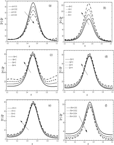
Figure 2. Pressure gradient $\frac{\mathrm{\partial }p}{\mathrm{\partial }x}$ versus x when $t=0.1$, $x=0.2$, $\lambda =10$, $k=0.1$, $a_{20}=2.0$, Pr = 6.9, A = 0.001, B = 2.0, Nt = 0.4, Nb = 0.4, Gr = 0.3, Qr = 0.3, Br = 2.0, $Q_0=2.0$; (g) $\varphi =0.6$, Q = 0.25. (h) M = 0.5,$\varphi =0.6$. (i) M = 0.5, Q = 0.25. (j) $\varphi =0.6$, Q = 0, Q = 0.25.

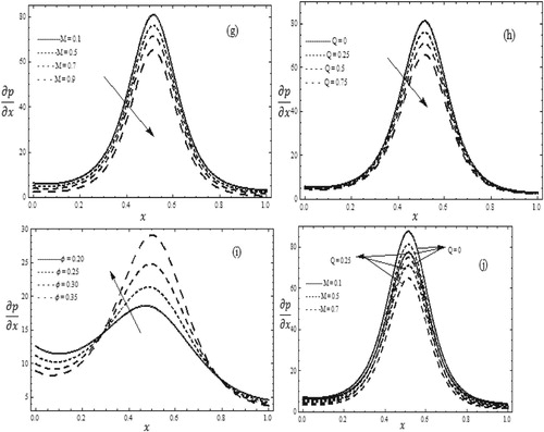
Figure 2(g) captures the effects of Hartman number M on the pressure gradient. Here it is observed that the pressure gradient is decreasing with the increase of M which is very helpful during heart surgery. Figure 2(h) includes flow rate Q the pressure gradient appears to decrease when Q is increased and it is observed that the pressure is maximum at zero flow rate. In Figure 2(i), the effect of amplitude ratio $\varphi$ on pressure gradient is plotted. The pressure gradient appears to increase when the amplitude ratio $\varphi$ increased. In Figure 2(j), the effect of flow rate Q and Hartman number M on pressure gradient is plotted. The pressure gradient decreases when the flow rate decreases and Hartman number also decreases.

4.2. Frictional force distribution

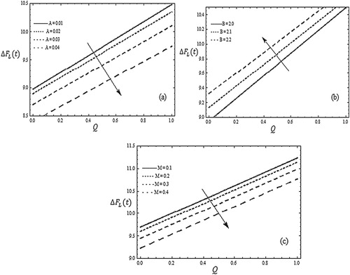
Figure 3 is plotted to show the behaviour of different parameters on the frictional force distribution. Figure 3(a) shows that the frictional force decreases with an increase in the Eyring–Powell fluid parameter A. Figure 3(b) shows that as Eyring–Powell fluid parameter B increases the frictional force increases. Figure 3(c) captures the effects of Hartman number M on the frictional force. Here it is observed that frictional force is a decreasing function of M.

Figure 3. Frictional force $\mathrm{\Delta }{F}_L\left(t\right)$ versus Q when $t=0.1$, $x=0.2$, $\lambda =10$, $k=0.1$, $a_{20}=2.0$, Pr = 6.9, Nt = 0.4, Nb = 0.4, Gr = 0.3, Qr = 0.3, Br = 2.0, $Q_0=2.0$, $\varphi =0.6$, Q = 0.25. (a) B = 2.0, M = 0.5. (b) A = 0.001, M = 0.5. (c) A = 0.001, B = 2.0.

4.3. Temperature distribution

Figures 4–5 are plotted to show the behaviour of different parameters on the temperature distribution $\theta$. Figure 4(a) shows that the temperature decreases with an increase in the Eyring–Powell fluid parameter A. Figure 4(b) shows the effect of Eyring–Powell fluid parameter B on frictional force. It is observed that the temperature appears to increase when B is increased. Figure 4(c) shows that the temperature increases with increasing of Hartman number. In Figure 4(d) is the effect joule heating $Q_0$. The temperature appears to increase when joule heating effect $Q_0$ increased.

Figure 4. Temperature $\theta$versus y when $t=0.1$, $x=0.2$, $\lambda =10$, $k=0.1$, $a_{20}=2.0$, Pr = 6.9, Nt = 0.4, Nb = 0.4, Gr = 0.3, Qr = 0.3, Br = 2.0, $\varphi =0.6$, Q = 0.25. (a) B = 2.0, M = 0.5, $Q_0=2.0$. (b) A = 0.001, M = 0.5,$Q_0=2.0$. (c) A = 0.001, B = 2.0, $Q_0=2.0$. (d) A = 0.001, B = 2.0, M = 0.5.

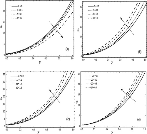
Figure 5. Temperature $\theta$ versus y when $t=0.1$, $x=0.2$, $\lambda =10$, $k=0.1$, $a_{20}=2.0$, A = 0.001, Q ₀= 2.0, $\varphi =0.6$, Q = 0.25. (e) Pr = 6.9, Nt = 0.4, Gr = 0.3, Qr = 0.3, Br = 2.0. (f) Pr = 6.9, Nb = 0.4, Gr = 0.3, Qr = 0.3, Br = 2.0. (g) Pr = 6.9, Nb = 0.4, Nt = 0.4, Qr = 0.3, Br = 2.0. (h) Pr = 6.9, Nb = 0.4, Nt = 0.4, Gr = 0.3, Br = 2.0. (i) Pr = 6.9, Nb = 0.4, Nt = 0.4, Gr = 0.3, Qr = 0.3. (j) Nb = 0.4, Nt = 0.4, Gr = 0.3, Qr = 0.3, Br = 2.0.

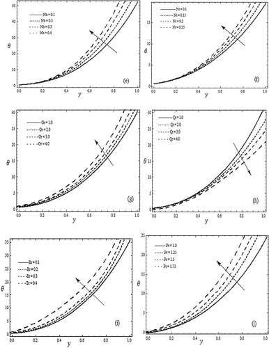
Figure 5(e) shows that the temperature increases with an increase in the Brownian motion parameter Nb. Figure 5(f) captures the effect of thermophoresis parameter Nt on the temperature, the temperature increases when the thermophoresis parameter increases. Figure 5(g) shows that as Grashof number Gr increases the temperature increases. Figure 5(h) includes the effect of local nanoparticle Grashof number Qr. Here temperature appears to decrease when Qr is increased. Figure 5(i) captures the effects of Brinkman number Br on the temperature. Here it is observed that temperature increases when Brinkman number Br increased. Figure 5(j) shows that the temperature increases with an increase in the Prandtl number Pr.

4.4. Concentration distribution

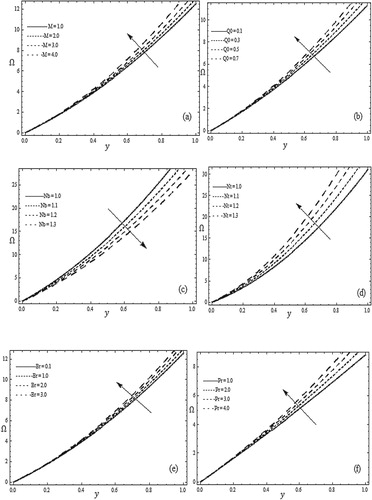
Figure 6 describes the variation of the concentration profile for several values of the Hartman number M, joule heating effect $Q_0$, thermophoresis parameter Nt and the Brownian motion parameter Nb, Brinkman number Br and Prandtl number Pr. In Figure 6(a), we observe that the concentration profile increases with an increase in Hartman number M. Figure 6(b) captures the effect of joule heating $Q_0$ on the concentration profile, the concentration increases when the joule heating effect $Q_0$increases. Figure 6(c) shows that the concentration profile decreases with an increase in Nb. Figure 6(d) captures the effect of thermophoresis parameter Nt on the concentration profile, the concentration increases when the thermophoresis parameter increased. Figure 6(e) includes the effect of Brinkman number Br on the concentration. Here it is observed that the concentration increases when Brinkman number Br increased. Figure 6(f) shows that the concentration increases with an increase in the Prandtl number Pr.

Figure 6. Concentration Ω versus y when $t=0.1$, $x=0.2$, $\varphi =0.6$, $\lambda =10$, $k=0.1$, $a_{20}=2.0$. (a) Pr = 6.9, Nb = 0.4, Nt = 0.4, Br = 2.0,Q₀= 0.5. (b) M = 0.5, Pr = 6.9, Nb = 0.4, Nt = 0.4, Br = 2.0. (c) Pr = 6.9, M = 0.5, Nt = 0.4, Br = 2.0,Q₀= 0.5. (d) Pr = 6.9, M = 0.5, Nb = 0.4, Br = 2.0, Q₀= 0.5. (e) Pr = 6.9, M = 0.5, Nb = 0.4, Nt = 0.4, Q₀= 0.5. (f) M = 0.5, Nb = 0.4, Nt = 0.4, Br = 2.0, $Q_0=0.5$.

5. Concluding remarks

Here we analysed the effect of joule heating on peristaltic blood flow of Eyring–Powell nanofluid in a non-uniform channel, is modelled in the presence of MHD, is studied under the assumptions of long wavelength and low Reynolds number. The results are discussed through graphs. We have the following main observations of the present analysis.

• Both pressure gradient and temperature distribution give opposite results with increasing values of Eyring–Powell fluid parameters A and B.

• Similar behaviour of pressure gradient and temperature profiles is observed with an increase in thermal Grashof number Gr. Also opposite behaviour of pressure gradient and temperature in the presence of local nanoparticle Grashof number Qr.

• Both pressure gradient and concentration profiles give opposite results with increasing values of Nt and Nb. Also the temperature increases with an increase in Brownian motion parameter Nb and thermophoresis parameter Nt.

• The pressure gradient decreases with increasing Hartman number M and flow rate Q.

• Pressure gradient decreases by increasing amplitude ratio $\varphi .$

• Frictional force gives the opposite behaviour with increasing values of Eyring–Powell fluid parameters A and B, also frictional force decreases with an increasing Hartman number M.

• Similar behaviour of temperature and concentration profiles increases in the presence of joule heating effect $Q_0$, Hartman number M, Brinkman number Br and Prandtl number Pr.

Acknowledgements

We would like to thank the editor and the reviewer’s for their constructive comments that significantly improved this manuscript.

Disclosure statement

No potential conflict of interest was reported by the authors.

ORCID

S. K. Asha http://orcid.org/0000-0001-6755-7629

G. Sunitha http://orcid.org/0000-0002-4949-5601

Additional information

Funding

This work was supported by the University Grant Commission (IN): [Grant Number 201718-NFST-KAR-01215 Dated: 01 April 2017]; University Grants Commission: [Grant Number F510/3/DRS-III/2016(SAP-I) Dated:29-Feb-2016].

Appendix

The values of a_11, a_12, a_14, a_13, a_15, a₁₆ in Equation (30) are given as $\begin{array}{rl}{a}_{11}& =\left(\frac{1}{3}+\frac{4F}{3h}\right)-M^2\left(\frac{1}{3}+\frac{4F}{3h}\right)y-\frac{P{y}^2}{2}\\ & -\left(4(1+B)\left(\frac{1}{3h^3}+\frac{F}{3h^4}\right)-\frac{Gr}{24h}-\frac{Qr}{24h}\right)y^3\\ & -576A\left(\frac{1}{3h^3}+\frac{F}{3h^4}\right)\frac{y^7}{7}.\end{array}$ $\begin{array}{rl}{a}_{12}& =(1+B)\left(\frac{1}{3}+\frac{4F}{3h}\right)-M^2\left(\frac{1}{3}+\frac{4F}{3h}\right)y-P{y}^2\\ & -\left(4(1+B)\left(\frac{1}{3h^3}+\frac{F}{3h^4}\right)-\frac{Gr}{24h}-\frac{Qr}{24h}\right)y^3\\ & -576A\left(\frac{1}{3h^3}+\frac{F}{3h^4}\right)\frac{y^7}{7}.\end{array}$ $\begin{array}{rl}{a}_{14}& =\frac{AP{M}^4}{4}{\left(\frac{1}{3}+\frac{4F}{3h}\right)}^2\frac{y^3}{6}+3A{M}^{2}P\left(\frac{1}{3}+\frac{4F}{3h}\right)\\ & \times \left((1+B)\left(\frac{1}{3h^3}+\frac{F}{3h^4}\right)-\frac{Gr}{24h}-\frac{Qr}{24h}\right)y^4\\ & +\left(A^{2}P{M}^2\left(\frac{1}{3}+\frac{4F}{3h}\right)+6A{M}^4{\left(\frac{1}{3}+\frac{4F}{3h}\right)}^2\right.\\ & \times \left.\left((1+B)\left(\frac{1}{3h^3}+\frac{F}{3h^4}\right)-\frac{Gr}{24h}-\frac{Qr}{24h}\right)\right)\frac{y^3}{6}\\ & +12AP\left((1+B)\left(\frac{1}{3h^3}+\frac{F}{3h^4}\right)-\frac{Gr}{24h}-\frac{Qr}{24h}\right)\frac{y^5}{5}\\ & +72A{M}^2\left(\frac{1}{3}+\frac{4F}{3h}\right)\left((1+B)\left(\frac{1}{3h^3}+\frac{F}{3h^4}\right)-\frac{Gr}{24h}\right.\\ & \left.-\frac{Qr}{24h}\right)\frac{y^5}{5}+288AP\left((1+B)\left(\frac{1}{3h^3}+\frac{F}{3h^4}\right)-\frac{Gr}{24h}\right.\\ & \left.-\frac{Qr}{24h}\right)\frac{y^6}{31}+576A\left((1+B)\left(\frac{1}{3h^3}+\frac{F}{3h^4}\right)-\frac{Gr}{24h}\right.\\ & {\left.-\frac{Qr}{24h}\right)}^2\frac{y^7}{7}+144A^2{M}^4\left(\frac{1}{3}+\frac{4F}{3h}\right)\left(\frac{1}{3h^3}+\frac{F}{3h^4}\right)\frac{y^7}{7}\\ & +72A^2{M}^{2}P\left(\frac{1}{3h}+\frac{F}{3h}\right)\left(\frac{1}{3h^3}+\frac{F}{3h^4}\right)y^8+64P{A}^2\\ & \times \left(\frac{1}{3h^3}+\frac{F}{3h^4}\right)y^9+1753A^2{M}^2\left(\frac{1}{3}+\frac{4F}{3h}\right)\\ & \left(\frac{1}{3h^3}+\frac{F}{3h^4}\right)\left((1+B)\left(\frac{1}{3h^3}+\frac{F}{3h^4}\right)-\frac{Gr}{24h}\right.\\ & \left.-\frac{Qr}{24h}\right)\frac{y^9}{3}+114061A^{2}P\left(\frac{1}{3h^3}+\frac{F}{3h^4}\right)\\ & \left((1+B)\left(\frac{1}{3h^3}+\frac{F}{3h^4}\right)-\frac{Gr}{24h}-\frac{Qr}{24h}\right)\frac{y^{10}}{90}\\ & +57984A^2\left(\frac{1}{3h^3}+\frac{F}{3h^4}\right)\left((1+B)\left(\frac{1}{3h^3}+\frac{F}{3h^4}\right)\right.\\ & \left.-\frac{Gr}{24h}-\frac{Qr}{24h}\right)\frac{y^{11}}{11}+165888A^3{M}^2\left(\frac{1}{3}+\frac{4F}{3h}\right)\\ & \times {\left(\frac{1}{3h^3}+\frac{F}{3h^4}\right)}^2\frac{y^{13}}{13}+2156544A^3{\left(\frac{1}{3h^3}+\frac{F}{3h^4}\right)}^2\frac{y^{14}}{91}\\ & +19795968A^3{\left(\frac{1}{3h^3}+\frac{F}{3h^4}\right)}^2\left((1+B)\left(\frac{1}{3h^3}+\frac{F}{3h^4}\right)\right.\\ & \left.-\frac{Gr}{24h}-\frac{Qr}{24h}\right)\frac{y^{15}}{335}+63700992A^4{\left(\frac{1}{3h^3}+\frac{F}{3h^4}\right)}^2\frac{y^{16}}{19}.\end{array}$ $\begin{array}{rl}{a}_{13}& =(1+B{)}^2\left(\frac{1}{3}+\frac{4F}{3h}\right)-M^2(1+B)\left(\frac{1}{3}+\frac{4F}{3h}\right)y\\ & -\left(P(1+B)+M^2(1+B)\left(\frac{1}{3}+\frac{4F}{3h}\right)\right)\frac{y^2}{2}\\ & +\left(\frac{M^4}{24}\left(\frac{1}{3}+\frac{4F}{3h}\right)-4(1+B)\left((1+B)\left(\frac{1}{3h^3}+\frac{F}{3h^4}\right)\right.\right.\\ & \left.\left.-\frac{Gr}{24h}-\frac{Qr}{24h}\right)\right)y^3+\frac{P{M}^2{y}^4}{144}\\ & +M^2\left((1+B)\left(\frac{1}{3h^3}+\frac{F}{3h^4}\right)\right.\\ & \left.-\frac{Gr}{24h}-\frac{Qr}{24h}\right)\frac{y^5}{5}-576A(1+B)\left(\frac{1}{3h^3}+\frac{F}{3h^4}\right)\frac{y^7}{7}\\ & +576M^{2}A\left(\frac{1}{3h^3}+\frac{F}{3h^4}\right)\frac{y^9}{63}.\end{array}$ $\begin{array}{rl}{a}_{15}& =Gr\frac{y^3}{6h}+Gr\left(Pr\frac{Nb}{2h^2}+Pr\frac{Nt}{2h^2}+Pr\frac{Q_0}{2}\right.\\ & \left.+Br{M}^2{\left(\frac{1}{3}+\frac{4F}{3h}\right)}^2\right)\frac{y^4}{12}-BrGr\left(\frac{1}{3}+\frac{4F}{3h}\right)\\ & \times \left(\frac{1}{3h^3}+\frac{F}{3h^4}\right)\frac{y^7}{840}.\end{array}$ $a_{16}=Qr\left(1+\frac{Nt}{Nb}\right)\frac{y^3}{6h}.$

The values of c_11, c_12, c_13, c_17, c_15, c_14, c₁₆ in Equation (32) are given as $\begin{array}{rl}{c}_{11}& =\left(\frac{1}{3}+\frac{4F}{3h}\right)h-M^2\left(\frac{1}{3}+\frac{4F}{3h}\right)\frac{h^2}{2}-\left(4(1+B)\right.\\ & \left.\times \left(\frac{1}{3h^3}+\frac{F}{3h^4}\right)-\frac{Gr}{24h}-\frac{Qr}{24h}\right)\frac{h^4}{4}\\ & -72A\left(\frac{1}{3h^3}+\frac{F}{3h^4}\right)\frac{h^8}{7}.\end{array}$ $\begin{array}{rl}{c}_{12}& =(1+B)\left(\frac{1}{3}+\frac{4F}{3h}\right)h-M^2\left(\frac{1}{3}+\frac{4F}{3h}\right)\frac{h^2}{2}\\ & -\left((1+B)\left(\frac{1}{3h^3}+\frac{F}{3h^4}\right)-\frac{Gr}{24h}-\frac{Qr}{24h}\right)h^4\\ & -72A\left(\frac{1}{3h^3}+\frac{F}{3h^4}\right)\frac{h^8}{7}.\end{array}$ $\begin{array}{rl}{c}_{13}& =(1+B{)}^2\left(\frac{1}{3}+\frac{4F}{3h}\right)h-M^2(1+B)\left(\frac{1}{3}+\frac{4F}{3h}\right)\frac{h^2}{2}\\ & -\left(M^2(1+B)\left(\frac{1}{3}+\frac{4F}{3h}\right)\right)\frac{h^3}{6}+\left(\frac{M^4}{24}\left(\frac{1}{3}+\frac{4F}{3h}\right)\right.\\ & \left.-(1+B)\left((1+B)\left(\frac{1}{3h^3}+\frac{F}{3h^4}\right)-\frac{Gr}{24h}-\frac{Qr}{24h}\right)\right)h^4\\ & +M^2\left((1+B)\left(\frac{1}{3h^3}+\frac{F}{3h^4}\right)-\frac{Gr}{24h}-\frac{Qr}{24h}\right)\frac{h^6}{30}\\ & -72A(1+B)\left(\frac{1}{3h^3}+\frac{F}{3h^4}\right)\frac{h^8}{7}\\ & +72M^{2}A\left(\frac{1}{3h^3}+\frac{F}{3h^4}\right)\frac{h^{10}}{630}.\end{array}$ $\begin{array}{rl}{c}_{17}& =\frac{A{M}^4}{4}{\left(\frac{1}{3}+\frac{4F}{3h}\right)}^2\frac{h^4}{24}+A{M}^2\left(\frac{1}{3}+\frac{4F}{3h}\right)\frac{h^4}{24}+5A{M}^2\\ & \times \left(\frac{1}{3}+\frac{4F}{3h}\right)\left((1+B)\left(\frac{1}{3h^3}+\frac{F}{3h^4}\right)-\frac{Gr}{24h}\right.\\ & \left.-\frac{Qr}{24h}\right)\frac{h^5}{5}+2A\left((1+B)\left(\frac{1}{3h^3}+\frac{F}{3h^4}\right)-\frac{Gr}{24h}\right.\\ & \left.-\frac{Qr}{24h}\right)\frac{h^6}{5}+288A\left((1+B)\left(\frac{1}{3h^3}+\frac{F}{3h^4}\right)-\frac{Gr}{24h}\right.\\ & \left.-\frac{Qr}{24h}\right)\frac{h^7}{217}+8A^2{M}^2\left(\frac{1}{3}+\frac{4F}{3h}\right)\left(\frac{1}{3h^3}+\frac{F}{3h^4}\right)h^{10}\\ & +114061A^2\left((1+B)\left(\frac{1}{3h^3}+\frac{F}{3h^4}\right)-\frac{Gr}{24h}-\frac{Qr}{24h}\right)\\ & \times \left(\frac{1}{3h^3}+\frac{F}{3h^4}\right)\frac{h^{11}}{990}+1099776A^3\\ & \times {\left(\frac{1}{3h^3}+\frac{F}{3h^4}\right)}^2\frac{h^5}{455}.\end{array}$ $\begin{array}{rl}{c}_{17}& =\frac{A{M}^4}{4}\left(\frac{1}{3}+\frac{4F}{3h}\right)\frac{h^4}{24}+A{M}^2\left(\frac{1}{3}+\frac{4F}{3h}\right)h^{4}24\\ & +5A{M}^2\left(\frac{1}{3}+\frac{4F}{3h}\right)\left((1+B)\left(\frac{1}{3h^3}+\frac{F}{3h^4}\right)\right.\\ & \left.-\frac{Gr}{24h}-\frac{Qr}{24h}\right)\frac{h^5}{5}+2A\left((1+B)\left(\frac{1}{3h^3}+\frac{F}{3h^4}\right)\right.\\ & \left.-\frac{Gr}{24h}-\frac{Qr}{24h}\right)\frac{h^6}{5}+288A\left((1+B)\left(\frac{1}{3h^3}+\frac{F}{3h^4}\right)\right.\\ & \left.-\frac{Gr}{24h}-\frac{Qr}{24h}\right)\frac{h^7}{217}+8A^2{M}^2\left(\frac{1}{3}+\frac{4F}{3h}\right)\\ & \times \left(\frac{1}{3^3}+\frac{F}{3h^4}\right)h^{10}+114061A^2\left((1+B)\left(\frac{1}{3h^3}+\frac{F}{3h^4}\right)\right.\\ & \left.-\frac{Gr}{24h}-\frac{Qr}{24h}\right)\left(\frac{1}{3h^3}+\frac{F}{3h^4}\right)\frac{h^{11}}{990}+1099776A^3\\ & \times \left(\frac{1}{3h^3}+\frac{F}{3h^4}\right)\frac{h^5}{455}\end{array}$ $\begin{array}{rl}{c}_{15}& =Gr\frac{b^3}{24}Gr\left(\text{Pr}\frac{Nb}{2h^2}+\text{Pr}\frac{Nt}{2h^2}+\text{Pr}\frac{Q_0}{2}+Br{M}^2{\left(\frac{1}{3}+\frac{4F}{3h}\right)}^2\right)\\ & \frac{h^5}{60}+Br\left(\frac{1}{3}+\frac{4F}{3h}\right)\left(\frac{1}{3h^3}+\frac{F}{3h^4}\right)\frac{h^8}{6720}.\end{array}$ $\begin{array}{rl}{c}_{14}& =6A{M}^4{\left(\frac{1}{3}+\frac{4F}{3h}\right)}^2\left((1+B)\left(\frac{1}{3h^3}+\frac{F}{3h^4}\right)-\frac{Gr}{24h}\right.\\ & \left.-\frac{Qr}{24h}\right)\frac{h^4}{4}+12A{M}^2\left(\frac{1}{3}+\frac{4F}{3h}\right)\left((1+B)\left(\frac{1}{3h^3}+\frac{F}{3h^4}\right)\right.\\ & \left.-\frac{Gr}{24h}-\frac{Qr}{24h}\right)\frac{h^6}{5}+72A\left((1+B)\left(\frac{1}{3h^3}+\frac{F}{3h^4}\right)-\frac{Gr}{24h}\right.\\ & {\left.-\frac{Qr}{24h}\right)}^2\frac{h^8}{7}+18A^2{M}^4\left(\frac{1}{3}+\frac{4F}{3h}\right)\left(\frac{1}{3h^3}+\frac{F}{3h^4}\right)\frac{h^8}{7}\\ & +1753A^2{M}^2\left(\frac{1}{3}+\frac{4F}{3h}\right)\left(\frac{1}{3h^3}+\frac{F}{3h^4}\right)\\ & \left((1+B)\left(\frac{1}{3h^3}+\frac{F}{3h^4}\right)-\frac{Gr}{24h}-\frac{Qr}{24h}\right)\frac{h^{10}}{30}\\ & +4832A^2\left(\frac{1}{3}+\frac{4F}{3h}\right)\left(\frac{1}{3h^3}+\frac{F}{3h^4}\right)\\ & \left((1+B)\left(\frac{1}{3h^3}+\frac{F}{3h^4}\right)-\frac{Gr}{24h}-\frac{Qr}{24h}\right)\frac{h^{12}}{11}\\ & +1237248A^3{\left(\frac{1}{3h^3}+\frac{F}{3h^4}\right)}^2\\ & \left((1+B)\left(\frac{1}{3h^3}+\frac{F}{3h^4}\right)-\frac{Gr}{24h}-\frac{Qr}{24h}\right)\frac{h^{16}}{335}\\ & +15925248A^4{\left(\frac{1}{3h^3}+\frac{F}{3h^4}\right)}^3\frac{h^{20}}{95}.\end{array}$ $c_{16}=Qr\left(1+\frac{Nt}{Nb}\right)\frac{h^3}{24}.$ The values of b_11, b_12, b_13, b_14, b₁₅ in Equation (33) are given as $\begin{array}{rl}{b}_{11}& =\frac{y}{h}+PrNb\frac{y^2}{2h^2}+PrNt\frac{y^2}{2h^2}+Pr{Q}_0\frac{y^2}{2}\\ & +Br{M}^2{\left(\frac{1}{3}+\frac{4F}{3h}\right)}^2\frac{y^2}{2}+2Br{M}^2\left(\frac{1}{3h^3}+\frac{F}{3h^4}\right)\frac{y^8}{7}\\ & -Br{M}^2\left(\frac{1}{3}+\frac{4F}{3h}\right)\left(\frac{1}{3h^3}+\frac{F}{3h^4}\right)\frac{y^5}{28}.\end{array}$ $\begin{array}{rl}{b}_{12}& =PrNb\frac{y^2}{2h^2}+PrNt\frac{y^2}{2h^2}+Pr{Q}_0\frac{y^2}{2}\\ & +Br{M}^2{\left(\frac{1}{3}+\frac{4F}{3h}\right)}^2\frac{y^2}{2}+Br{M}^2\left(\frac{1}{3h^3}+\frac{F}{3h^4}\right)\frac{y^8}{4}\\ & -Br{M}^2\left(\frac{1}{3}+\frac{4F}{3h}\right)\left(\frac{1}{3h^3}+\frac{F}{3h^4}\right)\frac{y^5}{20}.\end{array}$ $\begin{array}{rl}{b}_{13}& =\frac{y^2}{2h^2}+PrNb\frac{y^3}{6h^2}+PrNt\frac{y^3}{6h^2}+Pr{Q}_0\frac{y^3}{6}\\ & +Br{M}^2{\left(\frac{1}{3}+\frac{4F}{3h}\right)}^2\frac{y^3}{6}+8Br{M}^2\left(\frac{1}{3h^3}+\frac{F}{3h^4}\right)\frac{y^9}{31}\\ & -Br{M}^2{\left(\frac{1}{3}+\frac{4F}{3h}\right)}^3\left(\frac{1}{3h^3}+\frac{F}{3h^4}\right)\frac{y^6}{120}.\end{array}$ $\begin{array}{rl}{b}_{14}& =\frac{y^2}{2h^2}+\left(Pr\left(\frac{Nb}{h^2}+\frac{Nt}{h^2}+Q_0\right)+Br{M}^2\left(\frac{1}{3}+\frac{4F}{3h}\right)\frac{y^9}{31}\right)\\ & \times \frac{y^4}{12}-{\left(Br{M}^2\left(\frac{1}{3}+\frac{4F}{3h}\right)\left(\frac{1}{3h^3}+\frac{F}{3h^4}\right)\right)}^2\frac{y^{10}}{1446}\\ & +32{\left(Br{M}^2\left(\frac{1}{3h^3}+\frac{F}{3h^4}\right)\right)}^2\frac{y^{16}}{127}+\frac{2}{h}\left(Pr\left(\frac{Nb}{h^2}+\frac{Nt}{h^2}\right.\right.\\ & \left.\left.+Q_0\right)+Br{M}^2\left(\frac{1}{3}+\frac{4F}{3h}\right)\right)\frac{y^3}{6}-\frac{2}{h}\left(Br{M}^2\left(\frac{1}{3}+\frac{4F}{3h}\right)\right.\\ & \left.\times \left(\frac{1}{3h^3}+\frac{F}{3h^4}\right)\frac{y^6}{120}\right)+\frac{20}{h}\left(Br{M}^2\left(\frac{1}{3h^3}+\frac{F}{3h^4}\right)\frac{y^9}{3}\right)\\ & +\left(Pr\left(\frac{Nb}{h^2}+\frac{Nt}{h^2}+Q_0\right)+Br{M}^2\left(\frac{1}{3}+\frac{4F}{3h}\right)\right)\\ & \times \left(Br{M}^2\left(\frac{1}{3}+\frac{4F}{3h}\right)\left(\frac{1}{3h^3}+\frac{F}{3h^4}\right)\frac{y^7}{84}\right)\\ & -16\left(Pr\left(\frac{Nb}{h^2}+\frac{Nt}{h^2}+Q_0\right)+Br{M}^2\left(\frac{1}{3}+\frac{4F}{3h}\right)\right)\\ & \left(Br{M}^2\left(\frac{1}{3h^3}+\frac{F}{3h^4}\right)\frac{y^7}{315}\right).\end{array}$ $\begin{array}{rl}{b}_{15}& =\frac{8A^2}{63}{\left(\frac{1}{3h^3}+\frac{F}{3h^4}\right)}^2{y}^8+(1+B)\left(\left(\frac{1}{h^3}+\frac{F}{h^4}\right)\right.\\ & {\left.+\frac{M^2}{15}\left(\frac{1}{h^3}+\frac{F}{h^4}+\frac{Gr}{120h}+\frac{Qr}{120h}\right)\right)}^2\frac{y^{10}}{9}\\ & +\frac{23328}{63282025}{A}^2\left(\frac{1}{h^3}+\frac{F}{h^4}\right)\frac{y^{18}}{34}-\frac{2}{3}A\left(\frac{1}{h^3}+\frac{F}{h^4}\right)\\ & \left((1+B)\left(\frac{1}{h^3}+\frac{F}{h^4}\right)+M^2\left(\frac{1}{h^3}+\frac{F}{h^4}+\frac{Gr}{120h}\right.\right.\\ & \left.\left.+\frac{Qr}{120h}\right)\right)\frac{y^6}{15}-\frac{288}{103415}{A}^2{\left(\frac{1}{h^3}+\frac{F}{h^4}\right)}^4{y}^{13}\\ & +\frac{648}{144781}A(1+B)\left(\left(\frac{1}{h^3}+\frac{F}{h^4}\right)+\frac{M^2}{15}\left(\frac{1}{h^3}+\frac{F}{h^4}\right.\right.\\ & \left.\left.+\frac{Gr}{120h}+\frac{Qr}{120h}\right)\right)\left(\frac{1}{h^3}+\frac{F}{h^4}\right)y^4.\end{array}$

References

- Latham TW. Fluid motion in a peristaltic pump. MS Thesis, M.I.T. Cambridge. (1966).
- Jaffrin MY, Shapiro AH. Peristaltic pumping. Ann Rev Fluids Mech. 1971;3:13–37. doi: 10.1146/annurev.fl.03.010171.000305
- Hayat T, Tanveer A, Yasmin H, et al. Effects of convective conditions and chemical reaction on peristaltic flow of Eyring–Powell fluid. Appl Bionics Biomech. 2014;11:221–233. doi: 10.1155/2014/385821
- Khan AA, Masood F, Ellahi R, et al. Mass transport on chemicalized fourth-grade propagating peristaltically through a curved channel with magnetic effects. J Mol Liq. 2018;258:186–195. doi: 10.1016/j.molliq.2018.02.115
- Bhatti MM, Zeenshan A, Ellahi R, et al. Mathematical modelling of heat and mass transfer effects on MHD peristaltic propulsion of two-phase flow througha Darcy–Brinckman–Forcheimer porous medium. Adv Powder Technol. 2018;29(5):1189–1197. doi: 10.1016/j.apt.2018.02.010
- Zeeshan A, Ijaz N, Abbas T, et al. The sustainable characteristic of BIO-Bi-phase flow of peristaltic transport of MHD Jeffrey fluid in the human body. Sustainability. 2018;10:1–17. doi: 10.3390/su10082671
- Asha SK, Sunita G. Effect of couple stress in peristaltic transport of blood flow by homotopy analysis method. AJST. 2017;12:6958–6964.
- Bhatti MM, Ellahi R, Zeeshan A. Study of variable magnetic field on the peristaltic flow of Jeffrey fluid in a non-uniform rectangular duct having compliant walls. J Mol Liq. 2016;222:101–108. doi: 10.1016/j.molliq.2016.07.013
- Choi SUS. Enhancing thermal conductivity of the fluids with nanoparticles. ASME Fluids Eng Div. 1995;231:99–105.
- Bhatti MM, Zeeshan A, Ellahi R. Simultaneous effects of coagulation and variable magnetic field on peristaltically induced motion of Jeffrey nanofluid containing gyrotactic microorganism. Microvasc Res. 2017;110:32–42. doi: 10.1016/j.mvr.2016.11.007
- Ellahi R, Alamri SZ, Basit A, et al. Structural impact of kerosene-Al2O3 nanoliquid on MHD Poiseuille flow with variable thermal conductivity. application of cooling process. J Mol Liq. 2018;264:607–615. doi: 10.1016/j.molliq.2018.05.103
- Tanveer A, Hayat T, Alsaadi F, et al. Mixed convection peristaltic flow of Eyring–Powell nanofluid in a curved channel with compliant walls. Comput Biol Med. 2017;82:71–79. doi: 10.1016/j.compbiomed.2017.01.015
- Prakash J, Sharma A, Tripathi D. Thermal radiation effects on electroosmosis modulated of ionic nanoliquids in biomicrofluidics channel. J Mol Liq. 2018;249:843–855. doi: 10.1016/j.molliq.2017.11.064
- Powell RE, Eyring H. Mechanism for the relaxation theory of viscosity. Nature. 1944;154:427–428. doi: 10.1038/154427a0
- Abbasi FM, Alsaedi A, Hayat T. Peristaltic transport of Eyring–Powell fluid in a curved channel. J Aerosp Eng 2014;27(6):1–7. doi: 10.1061/(ASCE)AS.1943-5525.0000354
- Asha SK, Sunitha G. Mixed convection peristaltic flow of a Eyring–Powell nanofluid with magnetic field in a non-uniform channel. JAMS. 2018;2(8):332–334.
- Noreen S, Qasim M. Peristaltic flow of MHD Eyring–Powell fluid in a channel. Eur Phys J Plus. 2013;128(91):1–10.
- Hayat T, Irfan Shah S, Ahmad B, et al. Effect of slip on peristaltic flow of Powell–Eyring fluid in a symmetric channel. Appl Bionics Biomech. 2014;11:69–79. doi: 10.1155/2014/867328
- Abbasi FM, Hayat T, Alsaedi A. Numerical analysis for peristaltic motion of MHD Eyring–Prandtl fluid in an inclined symmetric cannel with inclined magnetic field. J Appl Fluid Mech. 2016;9:389–396. doi: 10.18869/acadpub.jafm.68.224.24158
- Hina S, Mustafa M, Hayat T, et al. Peristaltic flow of Powell–Eyring in curved channel with heat transfer: a useful application in biomedicine. Comput Methods Programs Biomed. 2016;135:89–100. doi: 10.1016/j.cmpb.2016.07.019
- Hayat A, Abdulhadi A. Influence of magnetic field on peristaltic transport for Eyring–Powell fluid in a symmetric channel during a porous medium. Math Theor Model. 2017;9:9–22.
- Ali Abbas M, Bai YQ, Rashidi MM, et al. Application of drug delivery in magnetohydrodynamics peristaltic blood flow of nanofluid in a non-uniform channel. J Mech Med Biol. 2016;16(04):1650052. doi: 10.1142/S0219519416500524
- Bhatti MM, Ali Abbas M, Rashidi MM. Combine effects of magnetohydrodynamics (MHD) and partial slip on peristaltic blood flow of Ree–Eyring fluid with wall properties. JESTECH. 2016;19(3):1497–1502.
- Zeeshan A, Bhatti MM, Akbar NS, et al. Hydromagnetic blood flow of sisko fluid in a non-uniform channel induced by peristaltic wave. CTP. 2017;68(1):103–110.
- Ranjit NK, Shit GC, Tripathi D. Joule heating and zeta potential effect on peristaltic blood flow through porous micro-vessels altered by elctrohydrodynamics. Microvasc Res. 2018;117:74–89. doi: 10.1016/j.mvr.2017.12.004
- Akbar NS, Nadeem S. Characteristics of heating scheme and mass transfer on the peristaltic flow for an Eyring–Powell fluid in an endoscope. Int Commun Heat Mass. 2012;55:375–383. doi: 10.1016/j.ijheatmasstransfer.2011.09.029
- Bhatti MM, Rashidi MM. Study of heat and mass transfer with joule heating on magnetohydrodynamic (MHD) peristaltic blood flow under the influence of hall effect. Propul Power Res. 2017;6(3):177–185. doi: 10.1016/j.jppr.2017.07.006
- Abbasi FM, Hayat T. Effects of inclined magnetic field and joule heating in mixed convective peristaltic transport of non-Newtonian fluids. Bull Pol Ac Tech. 2015;63(3):501–514.
- Hayat T, Aslam N, Rafiq M, et al. Hall and joule heating effects on peristaltic flow of Powell–Eyring liquid in an inclined symmetric channel. Results Phys. 2017;7:518–528. doi: 10.1016/j.rinp.2017.01.008
- Turkyilmazoglu M. A note on the homotopy analysis method. Appl Math Lett. 2010;23:1226–1230. doi: 10.1016/j.aml.2010.06.003
- Gupta VG, Gupta S. Application of homotopy analysis method for solving nonlinear Cauchy problem. Surv Math Appl. 2012;7:105–116.
Appendix
The values of a11, a12, a14, a13, a15, a16 in Equation (30) are given as
The values of c11, c12, c13, c17, c15, c14, c16 in Equation (32) are given as
The values of b11, b12, b13, b14, b15 in Equation (33) are given as